et de la Recherche Scientifique Universit´e Hadj Lakhdar Batna
Facult´e de Technologie
Th`ese Pr´esent´ee au
D´epartement d’Electronique Pour l’obtention du diplˆome de Doctorat en Sciences en Electronique
Par Fouzi DOUAK
Th`eme:
High-dimensional data analysis using
artificial intelligence methods
Devant le jury:
Dr. Ahmed Louchene Professeur U. de Batna Pr´esident
Dr. Nabil Benoudjit Professeur U. de Batna Rapporteur
Dr. Farid Melgani Professeur U. de Trento (Italie) Co-rapporteur
Dr. Khaled Melkemi Professeur U. de Biskra Examinateur
Dr. Noureddine Gol´ea Professeur U. de Oum El Bouaghi Examinateur Dr. R´edha Benzid Maˆıtre de Conf´erences (A) U. de Batna Examinateur
(2013)
Cette th`ese a ´et´e r´ealis´ee dans le cadre du programme Erasmus Mundus Averro`es financ´e par la Commission Europ´eenne.
applied in two main practical fields, which are the chemometrics, and Renewable energies fields. In particular, in the last few years, spectroscopy has represented an important technology for product analysis and quality control in different chemical fields. For example, it has been applied successfully in pharmaceutical, food and textile industries.
Another very interesting field is related to renewable energies. Renewable energies have been of great interest in recent years, as a consequence of increasing population and higher consumption of energy by developing countries, oil resources, natural gas and uranium will be depleted within a few decades. The unavoidable alternative becomes thus the development of renewable energy sources like solar energy, geothermal and wind power. In fact, the best use of renewable energies is an essential factor of development for all countries.
Machine learning methods exhibit the attractive advantage that they can provide very accurate predictors. In this thesis, we concentrate our study on two different methodologies:
In the first one, we propose a two-stage regression approach, which is based on the residual based correction concept (RBC) applied in chemometrics field, in order to improve the accuracy with respect to the single regressor. A comparative study with another approach which exploits differ-ently estimation errors, namely adaptive boosting for regression (AdaBoost.R), is also included. The idea in our proposed method is to correct any adopted regressor, called functional estimator, by analyzing and modeling its residual errors directly in the feature space. RBC is therefore not a regressor but a correction method, whose aim is not to reach the best achievable accuracy for a given data set but to possibly improve the estimation model of a given regressor.
In the second one, the regression process is undertaken by assuming that the training set is com-posed of a sufficient number of samples in order to obtain reliable and accurate estimations. However, from a practical point of view, the process of collecting training samples is not trivial, because the concentration/wind speed measurements associated with the spectral data have to be performed manually by human experts and thus are subject to errors and costs in terms of time and money. For this reason, the number of available training samples is typically limited and performances can be consequently affected due to data scarcity. A solution to this problem is given by active learning in this thesis. Active learning represents an interesting approach pro-posed in the literature to address the problem of training sample collection, in which training samples are selected in an iterative way in order to minimize the number of involved samples and the intervention of human users.
The experimental results on different real data sets show the effectiveness of the proposed solu-tions.
Keywords: Spectrometric data analysis, Renewable energy, Wind speed prediction, Residual-based correction (RBC), Boosting, Active learning, Regression.
Dans cette th`ese, de nouvelles m´ethodes d’apprentissage pour des probl`emes de r´egression sont propos´ees et appliqu´ees dans deux grands domaines ´a savoir la chimiom´etrie et l’´energie re-nouvelable. En particulier, au cours des derni`eres ann´ees, la spectroscopie a repr´esent´e une technologie importante pour l’analyse des produits et le contrˆole de qualit´e dans les diff´erents domaines de chimie. Par exemple, il a ´et´e appliqu´e avec succ`es dans les industries pharmaceu-tique, alimentaire et textile.
L’´energie renouvelable, a fait l’objet d’un grand int´erˆet au cours des derni`eres ann´ees, par cons´equence de la croissance d´emographique et l’augmentation de la consommation d’´energie par les pays en voie de d´eveloppement, les ressources en p´etrole, gaz naturel et uranium seront ´epuis´ees d’ici quelques d´ecennies. La solution in´evitable devient ainsi le d´eveloppement de sources d’´energie renouvelables comme l’´energie solaire, g´eothermique et ´eolienne. En fait, la meilleure utilisation des ´energies renouvelables est un facteur essentiel du d´eveloppement pour tous les pays.
Les m´ethodes d’apprentissage pr´esentent l’avantage attrayant qu’elles puissent fournir des pr´edic-teurs tr`es pr´ecis. Dans cette th`ese, nous nous concentrons notre ´etude sur deux diff´erentes m´ethodologies :
Premi`erement, nous proposons une approche de r´egression en deux ´etapes, qui est bas´e sur le con-cept de la correction de l’erreur r´esiduelle (RBC) appliqu´ee dans le domaine de la chimiom´etrie, afin d’am´eliorer la pr´ecision par rapport `a un r´egresseur unique. Une ´etude comparative avec une autre approche qui exploite diff´eremment les erreurs d’estimation, `a savoir le Boosting (Ad-aBoost.R), est ´egalement ´etudi´ee. L’id´ee de la m´ethode propos´ee est de corriger tout r´egresseur, appel´e estimateur fonctionnel, par l’analyse et la mod´elisation de ses erreurs r´esiduelles directe-ment dans l’espace des caract´eristiques. RBC n’est donc pas un r´egresseur, mais une m´ethode de correction, dont le but n’est pas d’atteindre la meilleure pr´ecision possible pour un ensemble de donn´ees, mais pour ´eventuellement am´eliorer le mod`ele d’´estimation pour un r´egresseur donn´ee. Deuxi`emement, le proc´ed´e de r´egression est effectu´e en supposant que l’ensemble d’apprentissage est constitu´e d’un nombre suffisant d’´echantillons afin d’obtenir des estimations fiables et pr´ecises. Cependant, d’un point de vue pratique, le processus de collecte d’´echantillons d’apprentissage n’est pas trivial, car les mesures de concentration / vitesse de vent associ´ees aux donn´ees doivent ˆetre effectu´ees manuellement par des experts humains et sont donc sujets `a des er-reurs et les coˆuts en termes de temps et d’argent. Pour cette raison, le nombre d’´echantillons d’apprentissage disponibles est g´en´eralement limit´e et les performances peuvent en ˆetre affect´ees en raison de la raret´e des donn´ees. Une solution `a ce probl`eme est donn´ee par l’apprentissage actif dans cette th`ese. L’apprentissage actif repr´esente une approche int´eressante propos´ee dans la litt´erature pour r´esoudre le probl`eme de la collecte des ´echantillons d’apprentissage, dans
Les r´esultats exp´erimentaux sur diff´erentes jeux de donn´ees r´eelles montrent l’efficacit´e des so-lutions propos´ees.
Mots-cl´es: Analyse des donn´ees de spectrom´etrie, ´Energie renouvelable, Pr´ediction de la vitesse du vent, Correction bas´ee sur r´esiduelle (RBC), Boosting, Apprentissage actif, R´egression.
First of all, I thank Allah, the Most High, for the opportunity He gave me to study, to research and to write this dissertation. Thanks Allah, my outmost thanks, for giving me the ability, the strength, attitude and motivation through this research and to complete this work.
I would like to express my most sincere gratitude to my advisor Prof. Nabil BENOUDJIT and to my co-advisor Prof. Farid MELGANI, for suggesting this area of research and for their solid technical guidance, continuous support and encouragement in my work. A special thanks is addressed to Prof. Farid MELGANI for his permanent availability and responsiveness to my requests and for giving his time and effort without reservation. I would also like to express my appreciation for their guidance during my study. Without which this research would never have reached this point.
I am indebted beyond measure to Prof. Nabil BENOUDJIT for giving me his inestimable ad-vices and valuable guidance during different cycles of my studies M.Sc and Dr.Sc. I have really learned a lot from his comments and suggestions.
I am also grateful to Prof. Khaled MELKEMI, Dr. Redha BENZID, Prof. Noureddine GOL´EA and Dr. Noureddine GHOGGALI who accepted to be my jury members, and devoted their precious time to review my thesis. I also want to thank Prof. Ahmed LOUCHENE for having agreed to preside this jury.
I would like to thank the Averro`es Erasmus Mundus program funded by the European Commission about 18 months in university of Trento. I wish to thank the members of the DISI -Dipartimento di Ingegneria e Scienza dell’Informazione, and more particularly to Dr. Edoardo PASOLLI, who have shared their knowledge and experiences with me. I extend additional thanks to Dr. Noureddine GHOGGALI. He has been a continual source of stimulation, help and very useful comments on all my work and most important a good friend. I would particularly like to thank Dr. Redha BENZID and Mr. Toufik BENTRCIA for their encouragement, help and support.
I would like to thank all my friends, colleagues and the staff at the Department of Electronics, University of Batna for their help along the realization of this work.
Finally, I am grateful to my parents, my brothers and my sister for their encouragement and continuous support.
Fouzi Douak
The work compiled in this thesis has been partially supported by the Averro`es Erasmus Mundus program funded by the European Commission (unfolding during the period of February 2011 to July 2012).
Contents
Page
Contents . . . iii
List of Tables . . . v
List of Figures . . . viii
List of Algorithms . . . ix
1 Introduction and Dissertation Overview 1 1.1 Context and motivations . . . 2
1.2 Problems and solutions . . . 4
1.3 Organization of the thesis . . . 8
2 Data Sets Description 10 2.1 Introduction . . . 11
2.2 Near infrared spectroscopy . . . 11
2.2.1 Relating absorbance to concentration . . . 13
2.2.2 High-dimensional data . . . 14
2.2.2.1 Orange juice . . . 15
2.2.2.2 Diesel . . . 16
2.2.2.3 Tecator . . . 18
2.3 Wind speed . . . 19
2.3.1 Nature of the wind . . . 19
2.3.2 Geographical variation in the wind resource . . . 20
2.3.3 Long-term wind speed variations . . . 21
2.3.4 Classification according to time horizons . . . 21
2.3.5 Wind prediction . . . 22
2.3.5.1 Physical approach . . . 23
2.3.5.2 Statistical approach . . . 23
2.3.5.3 Machine learning approach . . . 23
2.3.6 Low-dimensional data . . . 24
2.3.6.2 Wind speed data sets in Algeria . . . 25
2.4 Conclusion . . . 31
3 Linear and Nonlinear Regression 32 3.1 Introduction . . . 33
3.2 Linear regression methods . . . 34
3.2.1 Linear regression . . . 34
3.2.1.1 Least squares (LS) . . . 34
3.2.1.2 Ridge regression (RR) . . . 36
3.2.2 Linear projection techniques . . . 37
3.2.2.1 Principal component regression (PCR) . . . 37
3.2.2.2 Partial least squares regression (PLS) . . . 38
3.3 Nonlinear regression methods . . . 40
3.3.1 Kernel ridge regression (KRR) . . . 40
3.3.2 Support vector regression (SVR) . . . 41
3.3.3 Radial basis function neural network (RBFN) . . . 43
3.4 Conclusion . . . 44
4 Residual Correction Concept for Spectroscopic Data Sets Regression 46 4.1 Introduction . . . 47
4.2 Adaptive boosting for regression (AdaBoost.R) . . . 47
4.3 Proposed residual regression . . . 49
4.3.1 Description . . . 49
4.3.2 Theoretical considerations . . . 50
4.4 Experimental results on spectroscopic data set . . . 52
4.4.1 Experimental design . . . 52
4.4.2 Results with RBC . . . 56
4.4.3 Results with AdaBoost.R . . . 63
4.5 Conclusion . . . 66
5 Active Learning Methods 68 5.1 Introduction . . . 69
5.2 Active learning . . . 69
5.3 Proposed active learning methods . . . 72
5.3.1 Proposed general active learning strategies . . . 73
5.3.1.1 Pool of regressors (PAL) . . . 73
5.3.1.2 Distance from the closest training sample (DAL) . . . 75
5.3.1.3 Residual regression (RSAL) . . . 75
5.3.2.1 Distance from the support vectors (SVR-DAL) . . . 77
5.4 Experimental design . . . 78
5.4.1 Experiments on spectroscopic data set . . . 79
5.4.1.1 Experimental results . . . 80
5.4.2 Experiments on wind speed data set . . . 86
5.4.2.1 Experimental results . . . 86
5.5 Conclusion . . . 98
6 Final Conclusions and Future Works 100 6.1 Contributions and conclusion . . . 101
6.2 Perspectives and future work . . . 102
List of Publications 104
List of Tables
2.1 Classification of different time horizons. . . 22 2.2 Information about the meteorological stations considered in the experiments. . . 27
4.1 NMSE achieved on the orange juice data set by the five regression methods im-plemented without and with residual based correction (RBC) . . . 62 4.2 NMSE achieved on the tecator data set by the five regression methods
imple-mented without and with residual based correction (RBC) . . . 62 4.3 Results in terms of NMSE and processing time achieved by adaptive boosting
regression (AdaBoost.R). . . 65 4.4 Results in terms of NMSE and statistical test (p-value) achieved by the regression
method, the proposed RBC approach and the best adaptive boosting regression method. . . 66
5.1 Data set information and experimental setup for the different data sets. . . 79 5.2 NMSE, Standard Deviation (STD), # latent variables, # support vectors
ob-tained for the PLSR, RR, KRR and the SVR on (a) the diesel, (b) the orange juice, and (c) the tecator data sets. . . 85 5.3 RMSE Standard Deviation (STD), MAE Standard Deviation (STD), NMSE
Standard Deviation (STD), computation times obtained by the KRR predictor on Tlemcen, Chlef and Alger data sets. . . 94 5.4 RMSE Standard Deviation (STD), MAE Standard Deviation (STD), NMSE
Standard Deviation (STD), computation times obtained by the KRR predictor on Annaba, Djelfa and Batna data sets. . . 95 5.5 RMSE Standard Deviation (STD), MAE Standard Deviation (STD), NMSE
Standard Deviation (STD), computation times obtained by the KRR predictor on El Oued and Ghardaia data sets. . . 96 5.6 RMSE Standard Deviation (STD), MAE Standard Deviation (STD), NMSE
Standard Deviation (STD), computation times obtained by the KRR predictor on Adrar and Tamanrasset data sets. . . 97
5.7 Average RMSE Standard Deviation (STD), Average MAE Standard Deviation (STD), Average NMSE Standard Deviation (STD), and average computation time obtained on the ten data sets. . . 98
List of Figures
1.1 Two Phases of Supervised Learning Algorithms. . . 2
1.2 Flow chart of a general system of information extraction from Near infrared spec-troscopy. . . 3
2.1 Regions of the electromagnetic spectrum. . . 12
2.2 Electromagnetic Spectrum. . . 13
2.3 Absorbance according concentration . . . 14
2.4 Near-infrared reflectance spectra of orange juice data set. . . 15
2.5 All the spectra of the orange juice data set. . . 16
2.6 Principal components analysis (Pc1-Pc2) of the orange juice data set. . . 16
2.7 High leverage spectra (after centering and reduction) from the diesel data set. . . 17
2.8 All the spectra of the diesel data set. . . 17
2.9 Principal components analysis (Pc1-Pc2) of the diesel data set. . . 17
2.10 Near-infrared spectra of tecator data set. . . 18
2.11 All the spectra of the tecator data set. . . 19
2.12 Principal components analysis (Pc1-Pc2) of the tecator data set. . . 19
2.13 Seasonal world wind resource map in January and July. . . 20
2.14 Algeria’s geographic location. . . 25
2.15 Geographical location of the meteorological stations considered in the experiments. 26 2.16 Daily wind speed behavior for Tlemcen station. The blue curve show the training samples, while the red curve show the test samples. . . 27
2.17 Daily wind speed behavior for (a) Chlef, (b) Alger and (c) Annaba stations. The blue curve show the training samples, while the red curve show the test samples. 28 2.18 Daily wind speed behavior for (a) Djelfa, (b) Batna and (c) El Oued stations. The blue curve show the training samples, while the red curve show the test samples. 29 2.19 Daily wind speed behavior for (a) Ghardaia, (b) Adrar and (c) Tamanrasset stations. The blue curve show the training samples, while the red curve show the test samples. . . 30
3.2 Example of ε-insensitive tube and error function used in the SVM-based regression technique. Filled squares data are support vectors. Hence, SVs can appear only
on the tube boundary or outside the tube. . . 42
3.3 Architecture of a Radial Basis Function Neural Network (RBFN). . . 44
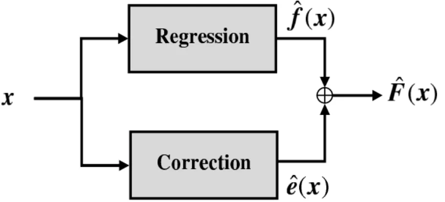
4.1 Block diagram illustrating the training phase of the residual correction. . . 50
4.2 Block diagram of the proposed approach in the global estimation phase. . . 50
4.3 NMSE k -fold cross-validation with respect to the number of selected variables, (a) orange juice and (b) tecator data set. . . 54
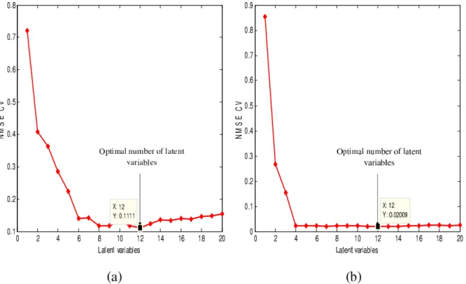
4.4 NMSE k -fold cross-validation with respect to the number of ℓv latent variables, (a) orange juice and (b) tecator data set. . . 55
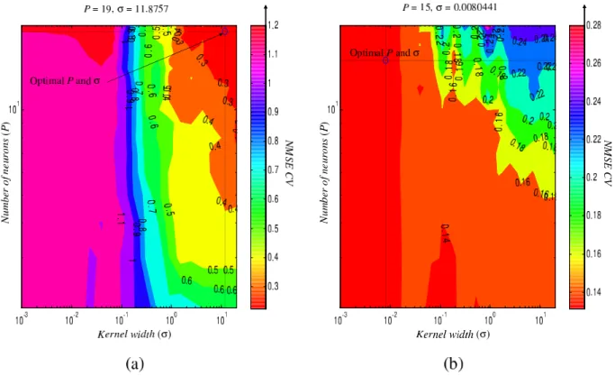
4.5 RBFN-Subset optimization number of neurons in hidden layer (P ) and the width parameter of the Gaussian kernel (σ) for the orange juice data set, (a) Regression and (b) Correction. . . 56
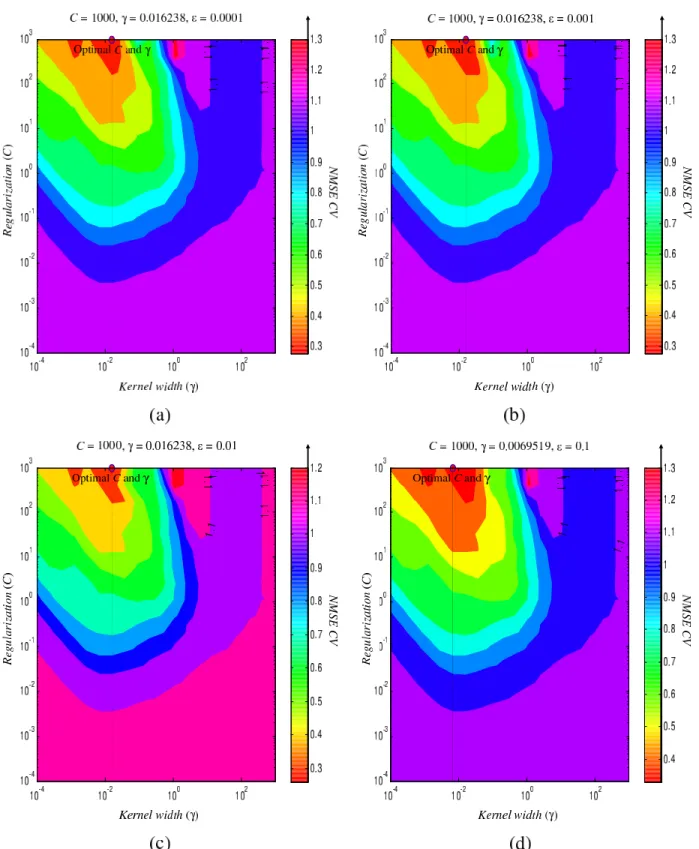
4.6 SVM-Subset optimization of parameters C, γ and ε for the orange juice data set in the case of Regression. (a) ε = 0.0001, (b) ε = 0.001, (c) ε = 0.01, and (d) ε = 0.1. . . 57
4.7 SVM-Subset optimization of parameters C, γ and ε for the orange juice data set in the case of Correction. (a) ε = 0.0001, (b) ε = 0.001, (c) ε = 0.01, and (d) ε = 0.1. . . 58
4.8 RBFN-All optimization number of neurons in hidden layer (P ) and the width parameter of the Gaussian kernel (σ) for the orange juice data set, (a) Regression and (b) Correction. . . 59
4.9 SVM-All optimization of parameters C, γ and ε for the orange juice data set in the case of Regression. (a) ε = 0.0001, (b) ε = 0.001, (c) ε = 0.01, and (d) ε = 0.1. 60 4.10 SVM-All optimization of parameters C, γ and ε for the orange juice data set in the case of Correction. (a) ε = 0.0001, (b) ε = 0.001, (c) ε = 0.01, and (d) ε = 0.1. 61 4.11 Behaviors of the Boosting-PLSR (linear, square and exponential) obtained by iterations for orange juice data set. . . 63
4.12 Behaviors of the Boosting (linear, square and exponential) obtained by iterations for subset orange juice data set. (a) Boosting-RBFN-Subset, (b) Boosting-SVM-Subset, (c) Boosting-RBFN-All, (d) Boosting-SVM-All. . . 64
5.1 Active learning cycle. . . 70
5.2 Performance example of regression. . . 71
5.3 Performance example of regression based active learning. . . 71
5.4 Flow chart of the proposed active learning approach. . . 73
5.5 Block diagram of the method based a pool active learning (PAL). . . 74
5.7 Performances achieved on the diesel data set for (a) PLSR, (b) RR, (c) KRR and (d) SVR in terms of NMSE and standard deviation. Each graph shows the results in function of the number of interactions. All results are averaged over ten runs of the approaches. (PLSR, RR, KRR, SVR)-Full = full, (PLSR, RR, KRR, SVR)-Random = random, (PLSR, RR, KRR, SVR)-PAL = pool of regressors, (PLSR, RR, KRR)-DAL = distance from the closest training sample in features space, SVR-DAL = distance from the support vectors. . . 81 5.8 Performances achieved on the orange juice data set for (a) PLSR, (b) RR, (c)
KRR and (d) SVR in terms of NMSE and standard deviation. . . 82 5.9 Performances achieved on the tecator data set for (a) PLSR, (b) RR, (c) KRR
and (d) SVR in terms of NMSE and standard deviation. . . 83 5.10 Illustration of learning samples, (a) 100 initial training samples, (b) 2419
unla-beled samples, respectively. . . 87 5.11 Illustration of selected samples. (a), (b) and (c) samples selected by PAL, DAL
and RSAL, respectively. . . 88 5.12 Example of active learning of (a) and (b) the evolution of sample selection at the
first to fourth iteration (100, 150, 200 and 250 training samples) by the PAL and DAL, respectively. . . 89 5.12 Example of active learning of (c) the evolution of sample selection at the first
to fourth iteration (100, 150, 200 and 250 training samples) by the RSAL. Each graph shows the results in function of the number of samples to add at each iteration (Ns). . . 90 5.13 Performances achieved by the investigated methods on the (a) Tlemcen and (b)
Chlef data sets in terms of RMSE and standard deviation of RMSE versus the number of selected samples. All results are averaged over ten runs. . . 91 5.14 Performances achieved by the investigated methods on the (a) Alger, (b) Annaba,
(c) Djelfa and (d) Batna data sets in terms of RMSE and standard deviation of RMSE versus the number of selected samples. . . 92 5.15 Performances achieved by the investigated methods on the (a) El Oued,(b) Ghardaia,
(c) Adrar and (d) Tamanrasset data sets in terms of RMSE and standard devia-tion of RMSE versus the number of selected samples. . . 93
List of Algorithms
1 AdaBoost.R . . . 48
2 The t − test for one-sided alternative hypothesis. . . 53
3 Resumes the general steps of the active learning approach. . . 72
4 Resumes the proposed methodology based on the pool of regressors. . . 74
5 Synthesizes the proposed strategy based on the distance from the closest training sample. . . 75
6 Synthesizes the proposed method based on the residual regression. . . 76
Introduction and Dissertation
Overview
Contents
1.1 Context and motivations . . . 2 1.2 Problems and solutions . . . 4 1.3 Organization of the thesis . . . 8
1.1
Context and motivations
In order to face the regression problem from a methodological viewpoint, several approaches to parameter estimation have been proposed. In this context, both linear and nonlinear regression methods have been proposed [1–4]. In the literature, one can find three very well-established approaches to envisage a regression task: 1) the supervised approach; 2) the unsupervised approach; and 3) the semi-supervised approach.
The supervised approach algorithm try to learn the input-output relationship f (x) by using a training data set X = [xi, yi], i = 1, ..., n, x ∈ ℜd where d is the feature space dimensionality and the labels y are discrete (y ∈ {1, ..., T }, T number of considered classes) for classification problems and real (y ∈ ℜ, continuous) value for regression tasks. The supervised learning problem is divided into two types, namely, classification (pattern recognition) and the regression (function approximation). In the regression problem, the task is to find the mapping between input x ∈ ℜd and output y. In this context, the learning task in regression is to find the underlying function between some d-dimensional input vectors xi and scalar outputs yi. There are two phases when applying supervised learning algorithms for problem-solving as shown in Figure 1.1. The first phase is so-called training phase where the learning algorithms design a mathematical model of a dependency, function or mapping in a regression or classification based on the training data given. While the second one is the test (application) phase, the parameters selecting (models developed) by the supervised approach are used to predict the outputs yi of the data which are unknown by the learning algorithms in the learning phase [5, 6].
Figure 1.1: Two Phases of Supervised Learning Algorithms.
In the unsupervised approach, there are only raw data xi ∈ ℜd, no labels data yi are available. Several algorithms to face this issue have been proposed, such as clustering techniques, principal
component analysis (PCA), and independent component analysis (ICA) [7–9].
Another method so-called semi-supervised learning can be considered as an attractive solution. Their underlying idea is to exploit unlabeled samples that are readily available at zero cost from the data sets under analysis, during the design of the regression model to compensate the deficit in labeled samples [10–13]. The cause of an appearance of the unlabeled data points is usually an expensive, difficult and slow process of obtaining labeled data. Thus, labeling brings additional costs and often it is not feasible. As a result, the goal of a semi-supervised learning algorithm is to predict the labels of the unlabeled data by taking the entire data set into account [5]. This thesis focuses firstly on the application of linear and nonlinear regression methods in the field of food industry (near infrared spectroscopy) and secondly on the wind prediction (renew-able energy) in different regions of Algeria.
In the last few years, the field of spectroscopy is continuously working on means to improve, optimize and gain a better understanding of the way food productions are run. The increased focus on food quality creates a big challenge for the industry into development and control of food productions. Ensuring the quality of food products needs monitoring and evaluation of every step from the raw material, to the production, to the final product, and in the distribu-tion [14]. A general system of informadistribu-tion-extracdistribu-tion from near infrared spectroscopy can be described by the block diagram shown in Figure 1.2.
Figure 1.2: Flow chart of a general system of information extraction from Near infrared spec-troscopy.
In the data-acquisition phase, modelling in laboratory where all measurements of variables must be carried out and where parameters of the model (linear or non-linear) must also be estimated. According on the reason of the application, the user may or may not be concerned in the spectral contributions originating from the physical characteristics of the sample. Where these charac-teristics are significant, the user may choose to work with the raw spectral data, otherwise some preprocessing is usually carried out [15]. Several spectral preprocessing methods exist, two cat-egories of the most widely used methods in data preprocessing are scatter correction methods and spectral derivatives (smoothing methods) [16].
In particular, automatic or semi-interactive calibration is a critical process monitoring and con-trol in real time as they provide the data from which relevant process and product information and conclusions should be extracted. Near Infrared spectroscopy is rich in information which is representative of both the physical and chemical characteristics of the sample, these characteris-tics have to be applied to take into account, for instance, pH, pressure, temperature, treatment that can removes or isolates the measurement sample in real time, etc. Recently, automatic ap-proaches to the analysis of spectroscopy data have attracted the attention of several researchers. This is a direct result of both the growing interest of end-users in the capabilities of spectroscopy and the scientific community’s realization that the automation of traditional “manual” analysis techniques (i.e., based on the intervention of human experts) offers great advantages in terms of time and economic cost. In this context, one of the main objectives of this dissertation is to provide a modest contribution to the automatic or semi-interactive techniques. Finally, the resulting preprocessed data can be fed to the analysis stage, which aims at extracting from the data set of spectroscopy information (product) being of interest to a given end user. In analytical chemistry, several linear calibration methods are applied to solve quantitative prob-lems with the argument that the relation between the chemical composition and the measured signal is linear [17]. However, there are many others where nonlinearity is present. In [18] discusses important sources of nonlinearity in near-infrared spectroscopy, namely :1) deviations from the Beer-Lambert law, which are typical of highly absorbing samples; 2) nonlinear detector responses; 3) drifts in the light source; 4) interactions between analytes; 5) nonlinearity between diffuse reflectance/transmittance data and chemical data. When the nonlinearity is significant, one can use truly nonlinear calibration techniques, for example, support vector machine (SVM).
The exploitation of renewable energy and especially of wind power is receiving increased at-tention the last years under the influence of novel guidelines adopted for energy management, and the concerns for global warming and climate change. In this framework the accurate esti-mation of the wind speed for short or long forecasting horizons is of primarily significance but not always easy to be attained due to the variable nature and the complexity of the environ-mental conditions that are implicated. In the literature, several wind speed prediction methods can be found. They can be divided into three categories: statistical methods [19–22], physical methods [19, 23], and machine learning methods including neural networks and support vec-tor machines since the estimation of the wind speed can be designed as a nonlinear regression problem [24–36].
1.2
Problems and solutions
The focus of this thesis is the development of models and algorithms for prediction. In this work, we concentrate our study on two well known issues of the machine learning community:
how to improve the prediction accuracy of a single regressor and how to deal with the issue of a limited labeled training samples.
Concerning the first issue, quality control of production systems and authenticity testing of products are increasing in importance in food industry, since they represent the new required issues to compete in the present-day market. Both production systems and food products can be described as complex systems, where several factors can interact and play a fundamental rule: consequently all these factors should be monitored and their synergic effects controlled. There is also a need in the food industry to rationalise and improve quality and process controls. The modern production systems require fast and automatic on-line monitoring, which should be able to extract the maximum amount of available information, in order to assure the opti-mal system functioning. On the other hand, food products acquire a higher value when their authenticity is protected, controlled and assured: in fact, consumers are more oriented towards purchasing food products of a certified origin. Consequently, during recent years there has been increasing interest in the origin authentication of food products, since authenticity can be often associated with food quality [37].
The use of traditional analytical techniques does not always match with these constraints, be-cause they can be time-consuming and expensive, while fast and cheap methods are essential, in order to assure a continuous monitoring. As a results novel analytical techniques have been used for these issues, since they enable more rapid and non-invasive characterisation of foods: nuclear magnetic resonance (NMR), near infrared spectroscopy (NIR), electronic sensors and image analysis are only a few of the involved analytical methods. A common property of these techniques is also the production of a large amount of spectra, so that several data sets are usually obtained and must be interpreted. Summarising, quality and authenticity control faces with complex systems, described by a large amount of data: hence, specific tools should be used in order to assure an effective prediction. Regression and classification can provide these specific tools: in the last years regression proved to be able to handle a huge amount of data, to process them, and to give useful results that can be explained by the users [38].
• In this context, in general all the three approaches (supervised, unsupervised and semi-supervised) use only a single regressor in order to estimate the prediction. However, using a single regressor usually is not capable of providing high accuracies over the entire input space. This is due to the fact that any estimator provides usually an accuracy depending on the region of the input space to which the analyzed pattern belongs to. In this dissertation a new method based on a residual-based correction (RBC) concept applied in chemometrics field. Its underlying idea is to correct any adopted regressor, called functional estimator, by analyzing and modeling its residual errors directly in the feature space. RBC is therefore not a regressor but a correction method, whose aim is not to reach the best achievable accuracy for a given data set but to possibly improve the estimation model of a given (poor or accurate) regressor. For this reason, we have proposed a regression approach that
consists in correcting a given estimator by exploiting its systematic errors in the feature space [39].
The second interesting field in this dissertation is renewable energy, as a consequence of increas-ing population and higher consumption of energy by developincreas-ing countries, oil resources, natural gas and uranium will be depleted within a few decades. The unavoidable alternative becomes thus the development of renewable energy sources like solar energy, geothermal and wind power. In fact, the best use of renewable energies is an essential factor of development for all countries. Algeria is a country rich in renewable energy resources, thanks to its geographical location and its large area which offer it great opportunities to find renewable energy sources (e.g., solar, wind, and geothermal) [40–42]. Focusing to the particular case of wind power, the estimation of wind speed in the short or the long-term represents an important target to evaluate the possi-bility to create new wind turbines or to predict the wind power production of existing ones [43]. Wind energy is seen as a green power technology for having less impacts on the environment. Wind energy plants generate no air pollutants or greenhouse gases. At the end of 2009, world-wide wind powered generators capacity was 159.2GW. All wind turbines installed worldworld-wide are generating 340 TWh/year, which is about 2 of worldwide electricity usage. Understanding the site-specific nature of wind is a critical phase in planning a wind energy project and detailed knowledge of wind on-site is needed to estimate the utility of a wind energy project [44]. The main reasons for invested and developed of renewable energies in Algeria are: 1) they con-stitute a solution economically viable to provide energy services to the rural isolated populations in particular in the Great South areas, where the demand consists essentially in satisfying basic energy requirements (light, refrigeration, television and radio), 2) they allow a sustainable devel-opment because of their inexhaustible character and of their limited impact on the environment (protection of the environment) and contribute to the safeguarding of our fossil resources, 3) the monetisation of these energy resources can have only positive repercussions as regards of regional balance and creation of jobs [45].
• In the aforementioned works, the regression process is undertaken by assuming that the training set is composed of a sufficient number of samples in order to obtain reliable and accurate estimations. However, from a practical point of view, the process of collecting training samples is not trivial, because the concentration/wind speed measurements have to be performed manually by human experts and thus are subject to errors and costs in terms of time and money. For this reason, the number of available training samples is typically limited and performances can be consequently affected due to data scarcity. A solution to this problem is given by semi-supervised approaches, in which the unlabeled samples are exploited during the design of the regression model in order to compensate for the deficit in labeled samples. By unlabeled samples, we mean samples whose spectral values are known,
but for which the corresponding concentration/wind speed values are unknown. In the data classification context, another solution to the problem of training sample collection is given by the active learning approach [46]. Starting from a small training set, additional samples are selected from a large amount of unlabeled data. These samples are labeled by the expert and added to the training set. The process is iterated until a stop criterion is reached. Active learning strategies have been applied successfully in different fields in classification [46–50]. Similarly, the active learning approach has been studied for regression problems by the machine learning and statistics communities, in which it is also known as optimal experimental design. After the seminal paper by Cohn et al. [51], in which active learning has been applied to two statistically-based learning architectures, such as mixtures of Gaussian and locally weighted regression, several works have appeared in the last few years. For instance, in [52], the authors focus on the problem of local minima in active learning for neural networks, and two probabilistic solutions are proposed. In [53], after introducing the fundamental limits in a minimax sense of active and passive learning for various function classes, some strategies based on a tree-structured partition of the data are presented. In [54], considering linear regression scenarios, a method using the weighted least squares learning based on the conditional expectation of the generalization error is proposed. In [55], the authors apply the query by committee approach in the regression context. The main idea is to train a committee of learners and query the labels of the samples where the committee’s predictions differ, thus minimizing the variance of the learner by training on samples where the variance is largest. In [56], solving the problems of active learning and model selection at the same time is suggested in order to improve further the generalization performance. In [57], a solution to the problem of pool-based active learning in linear regression is proposed. In [58], the authors develop a strategy for kernel-based linear regression, in which the proposed greedy algorithm employs a minimum-entropy criterion, derived using a Bayesian interpretation of RR. Note that while semi-supervised methods integrate unlabeled samples automatically (without the intervention of human experts) in the learning process, active learning works differently. Indeed, its aim is to minimize the number of unlabeled samples to be labeled by human experts. For such a purpose, it resorts to smart strategies for selecting the most significant unlabeled samples, that is, those which, if labeled, would most improve the classification/regression model. For this reason, the second objective of this dissertation is to propose new methodologies of active learning in different application fields. In particular, two main fields have been considered, namely chemometrics [59,60], and wind speed prediction [61]. Our motivation and contribution in this dissertation is that the active learning has not yet been explored for these two fields of interest.
1.3
Organization of the thesis
This thesis is organized into six chapters. In Chapter 2, we present the background information about the utilized data sets, in order to better understand the work present in this dissertation. Specifically, we use two different field data sets: 1) near infrared spectroscopy data sets, and 2) wind speed data sets. In Chapter 3, we present briefly the different methods of linear and non-linear regression that we use in this dissertation. In Chapter 4, we propose a two-stage regression approach, which is based on the residual correction concept. Its underlying idea is to correct any given regressor by analyzing and modeling its residual errors in the input space. We report and discuss results of experiments conducted on two different data sets in infrared spectroscopy and designed in such a way to test the proposed approach by: 1) varying the kind of adopted regression method used to approximate the chemical parameter of interest. Partial least squares regression (PLSR), support vector machine (SVM) and radial basis function neu-ral network (RBF) methods are considered; 2) adopting or not a feature selection strategy to reduce the dimension of the space where to perform the regression task. A comparative study with another approach which exploits differently estimation errors, namely adaptive boosting for regression (AdaBoost.R), is also included. In Chapter 5, we introduce an active learning approach for the estimation of chemical concentrations from spectroscopic data. Its main ob-jective is to opportunely collect training samples in such a way as to minimize the error of the regression process while minimizing the number of training samples used, and thus to reduce the costs related to training sample collection. In particular, we propose two different active learning strategies, developed for regression approaches, based on partial least squares regres-sion (PLSR), ridge regresregres-sion (RR), kernel ridge regresregres-sion (KRR) and support vector regresregres-sion (SVR). The first strategy is based on adding samples that are distant from the current training samples in the feature space, while the second one uses a pool of regressors in order to select the samples with the greatest disagreements among the different regressors of the pool. For SVR, a specific strategy based on the selection of the samples distant from the support vectors is proposed. Similarly, in the active learning approach is used for regression problems in the renewable energy field. In particular, we consider the problem of the estimation of wind speed in Algeria. In this case, the proposed strategies are specifically developed for kernel ridge regression (KRR). In particular, we propose three different active learning strategies. The first strategy uses a pool of regressors, while the second one relies on the idea to add samples that are distant from the available training samples, and the last strategy is based on the selection of samples which exhibit a high expected prediction error. Finally, general conclusions on the methodologi-cal and experimental developments conveyed by the present dissertation are drawn in Chapter 6.
The main contributions of the thesis are:
1. with respect to design of the regressors [39]:
• A new correction method for spectroscopy data set using linear and nonlinear regres-sion is proposed.
2. with respect to the problem of training sample collection [59–62]:
• In order to use and to improve forecasting/concentration systems, the quality of the predictions has to be evaluated, where “quality” and “quantity” refer to a judgement of how good or bad the prediction. In the case of data sets such as wind speed or spectroscopy, the easiest way to get an idea of the quality and quantity sample collection of this data sets is by using the active learning.
• We investigate and develop different techniques and methods for the active learning of spectroscopy and wind speed data sets. In particular, we address several issues associated to different regression tasks of data sets (supervised and unsupervised strategies).
Data Sets Description
Contents
2.1 Introduction . . . 11 2.2 Near infrared spectroscopy . . . 11 2.2.1 Relating absorbance to concentration . . . 13 2.2.2 High-dimensional data . . . 14 2.2.2.1 Orange juice . . . 15 2.2.2.2 Diesel . . . 16 2.2.2.3 Tecator . . . 18 2.3 Wind speed . . . 19 2.3.1 Nature of the wind . . . 19 2.3.2 Geographical variation in the wind resource . . . 20 2.3.3 Long-term wind speed variations . . . 21 2.3.4 Classification according to time horizons . . . 21 2.3.5 Wind prediction . . . 22 2.3.5.1 Physical approach . . . 23 2.3.5.2 Statistical approach . . . 23 2.3.5.3 Machine learning approach . . . 23 2.3.6 Low-dimensional data . . . 24 2.3.6.1 Geographic location of Algeria . . . 24 2.3.6.2 Wind speed data sets in Algeria . . . 25 2.4 Conclusion . . . 31
2.1
Introduction
In this chapter, we give an overview of some data sets used in the following chapters. The goal here is to give all the necessary information to understand the work presented in this thesis. In particular, two main fields have been considered, namely chemometrics, and renewable energy. The first field is the chemometrics data, and more particularly the spectral data, which is a high-dimensional data. Spectra are obtained from the analysis of the absorbance or reflectance of the light at different wavelengths on physical or chemical products. The objective of spectral analysis it to estimated a chemical parameters from product. The second field data set is considered as a low-dimensional data. The renewable energy (wind speed data) depends on meteorological variables such as relative humidity, temperature, etc. We use the data collected from ten stations located in Algeria. In each station, different physical input parameters, such as temperature measurements and average relative humidity, which in turn provides in output an estimate of the mean wind speed (m/s). We are interested in long term wind prediction in Algeria.
Depending on the applied fields, some other information can be needed in order to develop a model.
The organization of this chapter is as follow. Section 2.2 describe the near infrared spectroscopy data sets, while in Section 2.3, we present the wind speed data sets. Finally, we finish by a conclusion.
2.2
Near infrared spectroscopy
Spectroscopy is an important technology for product analysis and quality control in different chemical fields. For example, it has been applied successfully in the pharmaceutical [63, 64], food [65] and textile industries [66]. Chemical analysis by spectroscopy relies on the fast ac-quisition of a large number of spectral data, which can be analyzed in order to yield accurate estimations of the concentration of the chemical component of interest in a given product. Chemometrics can be defined as the chemical discipline that uses the methods and theory devel-oped in mathematical, statistical, and computer sciences to design or select optimal measurement procedures and experiments, and to provide maximum relevant chemical information by analyz-ing chemical data [16, 67, 68].
In analytical chemistry infrared spectroscopy (IR) is mainly used for the analysis of organic com-ponents. The qualitative assessment of organic components is performed for the identification of unknown compounds, or for the determination of the chemical structure of the components. In addition, IR analysis may be used for quantification of the components. IR spectroscopy is also known as vibration spectroscopy, since the spectra arise from transitions between the vibra-tional energy levels of a covalent bond of a molecule. The infrared spectrum, which ranges from 1 µm to 1000 µm, is part of the electromagnetic spectrum and is surrounded by the visible and
microwave regions (Figure 2.1). The IR region may be further subdivided in the near infrared, the Mid infrared and the Far infrared regions [69]. The NIR spectroscopy region is between 700-2500 nm (14300-4000 cm−1). Mid infrared and Far infrared light can be situated in the 2500-10,000 nm and 10-1000 µm range, respectively.
The instruments that measure electromagnetic radiation have several concepts and components in common. Shared instrumental components are discussed in some detail in a later section. Photometric instruments measure light intensity without consideration of wavelength. Most instruments today use filters (photometers), prisms, or gratings (spectrometers) to select (iso-late) a narrow range of the incident wavelength. Radiant energy that passes through an object will be partially reflected, absorbed, and transmitted. Electromagnetic radiation is described as photons of energy traveling in waves. The relationship between wavelength and energy E is described by Planck’s formula [70]:
E = hv, (2.1)
where h is a constant (6.62 × 10⁻²⁷ erg sec), known as Planck’s constant, and v is frequency. Because the frequency of a wave is inversely proportional to the wavelength, it follows that the energy of electromagnetic radiation is inversely proportional to wavelength. Figure 2.2 shows this relationship. Electromagnetic radiation includes a spectrum of energy from short-wavelength, highly energetic gamma rays and X-rays on the left in Figure 2.1 to long-wavelength radio frequencies on the right. Visible light falls in between, with the color violet at 400-nm and red at 700-nm wavelengths being the approximate limits of the visible spectrum [70].
Figure 2.2: Electromagnetic Spectrum.
2.2.1 Relating absorbance to concentration
Spectroscopy deals with the interaction of electromagnetic radiation with matter. Depending on the energy of the electromagnetic radiation, different oscillations are excited. This excita-tion involves absorpexcita-tion of the corresponding energy of the oscillaexcita-tion involved. For example, microwave radiation excites rotational motions of the molecules, infrared radiation excites vibra-tional modes, near-infrared radiation excites overtones and combination frequencies, ultraviolet and visible radiation excite electronic transitions [71]. Spectroscopic methods used within the food industry include ultraviolet and visual spectroscopy, fluorescence spectroscopy, nuclear magnetic resonance, microwave absorption, ultrasound transmission, and infrared techniques such as IR and NIR, and Raman spectroscopy covering most regions of the electromagnetic spectrum (see Figure 2.1). In the present thesis the spectroscopic technique have been applied is Near infraRed spectroscopy (NIR) (see Chapter 4 and Chapter 5). The relationship between absorbance and concentration is given by the Lambert-Beer’s Law:
A = M cd, (2.2)
where A is the absorbance, M is the molar absorptivity, c is the concentration, and d is the sample path length.
In a more practical sense, the absorbance is defined as the negative logarithm of the transmit-tance. This is given mathematically as:
A = − log T = − log I I0
, (2.3)
where I is the intensity of the light beam on the sample, I0is the intensity of the light beam after having passed the sample and T is transmittance. In infrared transmittance the relationship between the absorbance and the concentration logT1 is described by the Beer-Lambert’s law, i.e. this relation is linear [72]. However, that law should not be applied to near-infrared diffuse reflectance logR1, because of the light scattering [73] and the light path length shortening [74], as shown in Figure 2.3.
Figure 2.3: Absorbance according concentration
2.2.2 High-dimensional data
In the past, high dimensionality used to mean four or five attributes. Nowadays, we have to deal with, comparatively, super high-dimensional data, described by thousands of attributes. Data are nowadays complex and high-dimensional. In scene analysis, face recognition, document cate-gorization, speech recognition, optical character recognition, spectral and hyperspectral analysis, and many others, one has to deal with data that are described by many attributes, and con-sequently described with high-dimensional. Each data element is thus viewed as a point in a vector space whose dimension is the number of numerical features necessary to describe each data element [75, 76]. Feature selection is a step of major importance for the high-dimensional data sets. Indeed, learning with high-dimensional data is generally a complicated task due to many undesirable facts denoted by the term curse of dimensionality. Among the various ap-proaches to feature selection, principal component analysis (PCA) is very popular method that is able to adapt to this problem of dimensionality were developed.
In case the number of variables p is larger than the number of observations n, if X contains more variables than observations (p >> n) its covariance structure can be estimated by means of a PCA. In general, PCA constructs a new set of k << p variables, called loadings, which are linear combinations of the original variables and which contain most of the information. These loading vectors span a k-dimensional subspace. Projecting the observations onto this subspace yields the scores ti which for all i = 1, ..., n satisfy [77]. In following are three data sets illustrative of the context and needs of high-dimensional data analysis (This section gives additional information about the near-infrared spectroscopy data sets used in the Chapter 4 and Chapter 5).
2.2.2.1 Orange juice
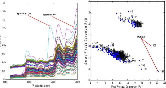
The first data set deals with the problem of determining sugar (saccharose) concentration in orange juice samples by near-infrared reflectance spectroscopy [78]. In this case, training (for model learning and selection) and test (for model assessment) sets contain respectively 149 and 67 samples, with 700 spectral variables that are the absorbance (log 1/R) at 700 wavelengths between 1100 and 2500 nm (where R is the light reflectance on the sample surface). The saccharose concentration ranges from 0 to 95.2% by weight. Figures 2.4-(a) and 2.4-(b) shows the spectra of orange juice used in the training and test sets, respectively. Figure 2.5 shows all the spectra of the orange juice data set. Both spectra 130 and 194 are considered as outliers in figure 2.5, where in Figure 2.6 gives a typical example of a score plot for two first principal components (Pc1-Pc2), after the application of the PCA on the 218 orange juice spectra. In Figure 2.6, two dense regions and few outliers can be seen, and we can consider that samples 130 and 194 are outliers, and can consequently be eliminated from the orange juice data set [79].
Figure 2.5: All the spectra of the orange juice data set.
Figure 2.6: Principal components analysis (Pc1-Pc2) of the orange juice data set.
2.2.2.2 Diesel
The second data set refers to multispectral acquisitions of diesel fuels [80]. It was built by the Southwest Research Institute in order to develop instrumentation to evaluate fuel on battle fields. Along with the spectral acquisitions, different properties are available, such as boiling point at 50% recovery, cetane number, density, freezing temperature, total aromatics and viscosity. The data set contains only summer fuels, and outliers were removed. In our experiments, we consider one of the most difficult prediction tasks in this data set, that is, the prediction of the cetane number of the fuel. All spectra range from 750 to 1550 nm, discretized into 401 wavelength values. The data set contains 20 high leverage spectra, shown in Figure 2.7-(a), and 225 low leverage spectra, the latter being separated into two subsets labeled a and b. As suggested by the providers of the data, we have built a learning set with the high leverage spectra and a subset of the low leverage spectra (thus yielding 133 spectra). Figure 2.7-(b) show the test set is made up of the low leverage spectra of subset b (gathering 112 spectra). In Figures 2.8 and 2.9 the all original spectra and their principal components analysis are shown. Note that the spectra look already pre-processed and no outlier was detected.
Figure 2.7: High leverage spectra (after centering and reduction) from the diesel data set.
Figure 2.8: All the spectra of the diesel data set.
Figure 2.9: Principal components analysis (Pc1-Pc2) of the diesel data set.
2.2.2.3 Tecator
The third data set deals with the determination of the fat content of meat samples analyzed by near infrared transmittance spectroscopy [81]. The spectra have been recorded on a Tecator In-fratec Food and Feed Analyzer working in the wavelength range 850-1050 nm. The spectrometer records light transmittance through the meat samples at 100 wavelengths in the specified range. The corresponding 100 spectral variables are absorbance defined by the measured transmittance. Each sample contains finely chopped pure meat with different moisture, fat and protein con-tents. Those contents, measured in percent by weight, are determined by analytic chemistry and range from 0.9 to 49.1%. The data set contains 172 training samples and 43 test samples (see Figure 2.10). The spectra are normalized according to the SNV method (standard normal variance, mean equal to zero and variance equal to 1). From the 215 original spectra, 2 outliers where detected. Figures 2.11 and 2.12 presents the all original spectra and the outlier detection procedure. It should be noted that the outliers detected in the tecator data set will not be eliminated [82].
Figure 2.11: All the spectra of the tecator data set.
Figure 2.12: Principal components analysis (Pc1-Pc2) of the tecator data set.
2.3
Wind speed
2.3.1 Nature of the windThe energy available in the wind varies as the cube of the wind speed, so an understanding of the characteristics of the wind resource is critical to all aspects of wind energy exploitation, from the identification of suitable sites and predictions of the economic viability of wind farm projects through to the design of wind turbines themselves, and understanding their effect on electricity distribution networks and consumers.
From the point of view of wind energy, the most striking characteristic of the wind resource is its variability. The wind is highly variable, both geographically and temporally. Furthermore this variability persists over a very wide range of scales, both in space and time. The importance of this is amplified by the cubic relationship to available energy. On a large scale, spatial variability describes the fact that there are many different climatic regions in the world, some much windier than others. These regions are largely dictated by the latitude, which affects the amount of insolation. Within any one climatic region, there is a great deal of variation on a smaller scale, largely dictated by physical geography the proportion of land and sea, the size of land masses, and the presence of mountains or plains for example. The type of vegetation may also have a significant influence through its effects on the absorption or reflection of solar radiation, affecting surface temperatures, and on humidity [43].
2.3.2 Geographical variation in the wind resource
The winds are driven almost entirely by the sun’s energy, causing differential surface heating. The heating is most intense on land masses closer to the equator, and obviously the greatest heating occurs in the daytime, which means that the region of greatest heating moves around the earth’s surface as it spins on its axis. Warm air rises and circulates in the atmosphere to sink back to the surface in cooler areas [43]. The tendency of climate remain which lead to clear climatic differences between regions. These differences are tempered by more local topographical and thermal effects [43,83]. The study of geographical distribution of wind speeds, characteristic parameters of the wind, topography and local wind flow and measurement of the wind speed are very essential in wind resource assessment for successful application of wind turbines [84]. The mountains and hills result in local regions of increased wind speed. This is partly a result of altitude - the earth’s boundary layer means that wind speed generally increases with height above ground, and hill tops and mountain peaks may ‘project’ into the higher wind-speed layers. It is also partly a result of the acceleration of the wind flow over and around hills and mountains, and funneling through passes or along valleys aligned with the flow. Equally, topography may produce areas of reduced wind speed, such as sheltered valleys, areas in the lee of a mountain ridge or where the flow patterns result in stagnation points [43]. For example, Figure 2.13 shows a geographical map of the distribution of wind speed in January and July.
The thermal effect is another important factor may also result in considerable local variations. Coastal regions are often windy because of differential heating between land and sea. This effect may also be produced by differences in altitude. Thus cold air from high mountains can sink down to the plains below, causing quite strong and highly stratified ‘downslope’ winds [43].
2.3.3 Long-term wind speed variations
There is evidence that the wind speed at any particular location may be subject to very slow long-term variations. Although the availability of accurate historical records is a limitation [85]. Clearly these may be linked to long term temperature variations for which there is ample historical evidence. There is also much debate at present about the likely effects of global warming, caused by human activity, on climate, and this will undoubtedly affect wind climates in the coming decades. Apart from these long-term trends there may be considerable changes in windiness at a given location from one year to the next. These changes have many causes. They may be coupled to global climate phenomena, changes in atmospheric particulate resulting from volcanic eruptions, and sunspot activity. These changes add significantly to the uncertainty in predicting the energy output of a wind farm at a particular location during its projected lifetime [43].
2.3.4 Classification according to time horizons
The various forecasting models in the literature can be different based on the forecasting hori-zons, which can vary according to the required application and the technique used. The fore-casting system is divided into four categories according to time horizons: very short term, short term, medium term, or long term. The time span is different in various literature descriptions. The specific classification is listed in Table 2.1, this table also presents the application for each prediction horizon [86, 87].
Table 2.1: Classification of different time horizons.
Time Horizon Range Application Purpose
Very short term
Few seconds to 30 minutes ahead • Electricity Market Clearing (in minutes) • Wind Turbine Control Short term
30 minutes to 48(or 72) hours ahead • Economic Load Dispatch Planning (in hours) • Load Increment/Decrement Decisions Medium term
48(or 72) hours to 1 week ahead
• Generator Online/Offline Decisions (in days) (Arrangements for Maintenance)
• Unit Commitment Decisions Long term
1 week to 1 year or more ahead
• Maintenance Scheduling to Obtain Optimal Operating Cost
(in years) • The Feasibility Study for Design of the Wind Farm
2.3.5 Wind prediction
In general, different methods are used for wind prediction. The easiest ones are based on clima-tology or averages of past production values. They may be considered as reference forecasting methods since they are easy to implement. The famous of these reference methods is certainly persistence. This is one of the simplest models. It is very effective for very short term fore-casting. It’s based on the idea that under similar conditions the next forecast data point will be approximately the same or constant to present data point value, due the simplicity, reduced complexity and low cost implementation. This model is very popular. However, this model suffer from a drawback, which is the larger the time horizon is the bigger the prediction error. Advanced approaches for wind power forecasting necessitate predictions of meteorological vari-ables as input. Then, they differ in the way predictions of meteorological varivari-ables are converted to predictions of wind power production, through the so-called power curve [43].
Wind power generation is directly linked to weather conditions and thus the first aspect of wind power forecasting is the prediction of future values of the necessary weather variables at the level of the wind farm. This is done by using numerical weather prediction (NWP) models. Such models are based on equations governing the motions and forces affecting motion of fluids. From the knowledge of the actual state of the atmosphere, the system of equations allows to estimate what the evolution of state variables, e.g. temperature, velocity, humidity and pressure, will be at a series of grid points. The meteorological variables that are needed as input for wind power prediction obviously include wind speed and direction, but also possibly temperature, pressure and humidity. The distance between grid points is called the spatial resolution of the NWPs. The main disadvantage of using this model is that the cost of implementation, complexity in-volved in it takes a long time in processing to train the model [88].
In the literature, several wind speed prediction methods can be found. They can be divided into three categories: physical methods, statistical methods, and machine learning methods.
2.3.5.1 Physical approach
It is based on a detailed physical considerations to predict the future wind speed like terrain, obstacle, pressure, and temperature. Sometimes they are only the first step to forecast the wind, which is supplied as auxiliary input of other statistical models. Numeric weather prediction (NWP) is developed by meteorologists for large-scale area weather prediction. NWP is a physical approach to wind forecasting, it is operate by solving complex mathematical models that use weather data [86, 89].
2.3.5.2 Statistical approach
The statistical approach is based on training with measurement data and uses difference between the predicted and the actual wind speeds in immediate past to tune model parameters, it is not based on any predefined mathematical model and rather it is based on statistical linear and nonlinear models [86, 90, 91].
2.3.5.3 Machine learning approach
Models based on machine learning techniques such as Artificial Neural Network (ANN), bayesian networks, fuzzy logic, support vector machine (SVM) and hybrid models, are used for the wind speed data in recent years, because of their excellent ability to learn non-linear relationships from experience, many researchers found these techniques to be effective for wind speed and power output prediction [24–36].
In this context, different architecture and types of artificial neural network is presented. For instance, Fadare [24] compared three different artificial neural networks (ANNs) applied to wind speed in Nigeria and used different configurations of the ANN. Li [92] investigated a method to do one-step-ahead prediction of wind power generation using recurrent multilayer perceptron neural networks (RMLP). Results showed that the RMLP model performed better in 1-hour prediction than that for 10-min prediction. In [25], three types of neural networks, namely, adaptive linear element, back propagation, and radial basis function, are compared. Mohan-des [29] used neural networks (ANN) to forecast the mean of monthly and daily wind speed. The forecasting accuracy was compared with the autoregressive (AR) model. The results indi-cated that the ANN model outperformed the AR model for all examined forecasting horizons. In [28], introduced the support vector machines (SVM) for wind speed prediction and compared it with the multilayer perceptron neural networks (MLP). The results proved that the SVM model is better than MLP model. In [33], hybridization of linear regression (MLR, SVM-linear) and nonlinear regression (ANN, SVM-Gaussian, SVM-polynomial). Sfetsos [93] examined and
compared various artificial intelligence based forecasting models based on time series analysis. The models examined in this study include ARMA models, feed-forward and recurrent neural networks, Adaptive Neuro-Fuzzy Inference Systems (ANFIS) and Neural Logic Networks (NLN). In [94], used an artificial neural network (ANN) to predict the average hourly wind speed and the related power production.
Among several nonlinear regression approaches, KRR, which is a kernel version of the ridge regression (RR), has a very good generalization performance by selecting the suitable regular-ization parameter [95]. The nonlinear maps can be approximated by means of kernel ridge regression, an extension of linear ridge regression based on kernel functions. KRR offers the advantage of being fast to evaluate, requiring only a single matrix inversion which depends on the number of points but is independent of the number of attributes in the input space [96]. The focus of this thesis lies on machine learning approach for wind speed prediction.
2.3.6 Low-dimensional data
Many data analysis borrowed from statistics or machine learning were designed for low-dimensional, large sample data, based on a scheme that the human mind can apprehend, in this case we do not need to features selection.
Let us consider a set of n training samples X = (x1, ..., xn) with xi = (xi1, ..., xid) represented in the d-dimensional feature space ℜd. In this section of wind speed data set, we assume in addition that the data are low-dimensional. Here, this means that d should at least be smaller than n (This section gives additional information about the wind speed data sets used in the Chapter 5).
2.3.6.1 Geographic location of Algeria
Algeria’s geographic location has several advantages for extensive use of most of the renewable energy (solar and wind). Algeria situated in the centre of North Africa between the 38-35◦
of latitude north and 8-12◦ longitude east, has an area of 2,381,741 km2 [97].
Administratively speaking, Algeria is divided into 48 provinces and lies, in the north, on the coast of the Mediterranean Sea. The length of the coastline is 2400 km. In the west Algeria borders with Morocco, Mauritania and occidental Sahara, in the southwest with Mali, in the east with Tunisia and Libya, and in the southeast with Niger (see Figure 2.14) [41].
Figure 2.14: Algeria’s geographic location.
2.3.6.2 Wind speed data sets in Algeria
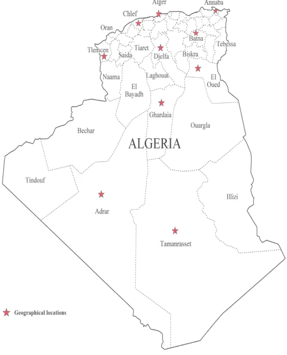
We used different wind speed data measurement stations distributed over the vast Algerian territory, which cover a period of ten years (between January 1st, 2001 to December 31st, 2010) based on ten different stations in Algeria, namely, Tlemcen, Chlef, Alger, Annaba, Djelfa, Batna, El Oued, Ghardaia, Adrar and Tamanrasset. These stations are distributed in different regions of the country as depicted in Figure 2.15.
Figure 2.15: Geographical location of the meteorological stations considered in the experiments.
Table 2.2 provides the exact location of these stations, their altitude as well as the related number of daily measurements used for training and testing the investigated methods. The month number, the day number (within the month), three temperature measurements (average, maximum and minimum temperatures) and the average relative humidity are used as input features for the prediction, which in turn provides in output an estimate of the mean wind speed.
Table 2.2: Information about the meteorological stations considered in the experiments.
Location Data set information
Name Latitude Longitude Altitude # training # test (m) samples samples (days) (days) Tlemcen 35.01 -1.46 247 2519 1095 Chlef 36.21 1.33 143 1679 961 Alger 36.76 3.1 12 965 1013 Annaba 36.83 7.81 4 2514 1090 Djelfa 34.33 3.25 1144 2401 1042 Batna 35.75 6.18 1052 2415 1086 El Oued 33.5 6.11 63 2473 954 Ghardaia 32.4 3.81 450 2486 1092 Adrar 27.88 -0.28 263 2262 1001 Tamanrasset 22.8 5.51 1364 2319 1087
For each station, the wind speed data set was divided into two sets: 1) a training set, from 1st January 2001 to 31st December 2007; and 2) a test set, from 1st January 2008 to 31st December 2010. Figures 2.16-2.19 illustrates ten different wind speed data sets used in the experimental analysis.
Figure 2.16: Daily wind speed behavior for Tlemcen station. The blue curve show the training samples, while the red curve show the test samples.
Figure 2.17: Daily wind speed behavior for (a) Chlef, (b) Alger and (c) Annaba stations. The blue curve show the training samples, while the red curve show the test samples.
Figure 2.18: Daily wind speed behavior for (a) Djelfa, (b) Batna and (c) El Oued stations. The blue curve show the training samples, while the red curve show the test samples.
Figure 2.19: Daily wind speed behavior for (a) Ghardaia, (b) Adrar and (c) Tamanrasset sta-tions. The blue curve show the training samples, while the red curve show the test samples.