Topology optimisation of electromagnetic devices

HAL Id: tel-01818091

https://tel.archives-ouvertes.fr/tel-01818091

Submitted on 3 Jul 2019

HAL is a multi-disciplinary open access archive for the deposit and dissemination of sci-entific research documents, whether they are pub-lished or not. The documents may come from teaching and research institutions in France or abroad, or from public or private research centers.

L’archive ouverte pluridisciplinaire HAL, est destinée au dépôt et à la diffusion de documents scientifiques de niveau recherche, publiés ou non, émanant des établissements d’enseignement et de recherche français ou étrangers, des laboratoires publics ou privés.

Bibi Safoorah Bilquis Mohamodhosen

To cite this version:

Bibi Safoorah Bilquis Mohamodhosen. Topology optimisation of electromagnetic devices. Electro-magnetism. Ecole Centrale de Lille, 2017. English. �NNT : 2017ECLI0028�. �tel-01818091�

CENTRALE LILLE

THESE

DOCTEUR

En

Spécialité : Génie Electrique Par

MOHAMODHOSEN Bilquis

DOCTORAT DELIVRE PAR CENTRALE LILLE

Titre de la thèse :

TOPOLOGY OPTIMISATION OF ELECTROMAGNETIC DEVICES OPTIMISATION TOPOLOGIQUE DE DISPOSITIFS ELECTROMAGNETIQUES

Soutenue le 6 décembre 2017 devant le jury d’examen : Président Betty Semail, Professeur, Polytech Lille

Rapporteur Frédéric Messine, Professeur, ENSEEIHT- Toulouse

Rapporteur Bruno Dehez, Professeur, Université Catholique de Louvain

Directeur de thèse Frédéric Gillon, Maître de Conférences HDR, Centralelille

Co-Directeur de thèse Abdelmounaïm Tounzi, Professeur, Université Lille 1

Membre Stéphane Vivier, Maître de Conférences HDR, UT Compiègne

Invité _{Jean-Claude Mipo, Société Valéo} Thèse préparée dans le Laboratoire L2EP avec le soutien financier de la Région Hauts-de-France

L’établissement Centrale Lille, le laboratoire L2EP, les encadrants de la thèse et moi-même remercions sincèrement la région Hauts-de-France pour le support financier apporté à ces travaux de recherche. Nous remercions également l’état français sans lequel ces travaux de recherche n’auraient pu être réalisés. Je remercie à titre personnel Centrale Lille et le L2EP de m’avoir donné l’opportunité de conduire ma thèse au sein de leur institution.

i

Topology Optimisation (TO) is a fast growing topic that has been sparking the interest of many researchers for the past two decades in the electromagnetic community. Its attractiveness lies in the originality of finding innovative structures without any layout a priori. This thesis work is oriented towards the TO of electromagnetic devices by elaborating on various aspects of the subject. First of all, a tool for TO is developed and tested, based on the ‘home-made’ tools available at the L2EP. As TO requires a FE and an optimisation tool working together, a coupling is done using both. Furthermore, a TO methodology is developed and tested, based on the Density Method. An academic cubic test case is used to carry out all the tests, and validate the tools and methodology. An approach is also developed to consider the nonlinear behaviour of the ferromagnetic materials with our TO tools. Afterwards, the methodology is applied to a 3D electromagnet, which represents a more real test case. This test case also serves to compare the results with linear and nonlinear behaviour of the materials used. Various topologies are presented, for different problem formulations. Subsequently, the methodology is applied to a more complex electromagnetic device: a Salient Pole Synchronous Generator. This example allows us to see how the problem definition can largely affect TO results. Some topologies are presented and their viability is discussed.

ii

The journey of a PhD student towards the glorious day of being awarded the title of Doctor is a long and strenuous one, during which the support and help of others is simply a sine qua non. I wholeheartedly seize this moment to express my gratitude and appreciation towards those who have fuelled my determination, or simply made the road more pleasant.

God, thank You for giving me all the grit I needed to pursue my dreams and attain my goals; You were inarguably the one who knew all of my ups and downs.

Before addressing some words to the people who have been there throughout my PhD, I would like to thank the members of the jury for making the defence day possible despite their numerous commitments. Thank you Pr. Frédéric Messine and Pr. Bruno Dehez for accepting the responsibility of rapporteur to my thesis, for your relevant suggestions and useful interrogations; Stephane Vivier (HDR) and Dr. Jean Claude Mipo for keeping a practical and industrial analysis to the discussion as jury members, and Pr. Betty Semail for her timely presiding of the jury.

I am very grateful to my two thesis directors, Pr. Frédéric Gillon and Pr. Mounaïm Tounzi, for trusting me in undertaking this thesis, which promised to be a challenging one since the very beginning. I can never forget their words of encouragement and conviction which led me to choose this path after my internship with them. I enjoyed working with Frédéric for his patience and passion in transmitting his knowledge to students, his availability, optimism, and invariably good humour. I have learned a lot working with Mounaïm as well who, despite not being on the same Centralelille premises, was always accessible whenever his help was needed. His pertinent analyses and comments have undoubtedly contributed to the good achievement of this work, without forgetting his humane and joyful character. I cannot fail to mention Loïc Chevallier, who has been a huge support during my PhD in terms of

code_Carmel development, utilisation and endless hours of debugging, and Julien Korecki for

providing helpful tips and information on the use of Salome with code_Carmel. In the same way, I am very grateful to Florent Delhaye for his efficient technical help in the utilisation, maintenance and update of Sophemis. I cannot forget the teaching staffs of Centralelille and Université Lille1 who have always provided valuable suggestions and advice whenever they were summoned, and also non-teaching staffs for their pleasant humour and administrative support. But the lively office ambience would not have been the same without my lab mates, whether they were here for a short or long term.

iii

stopped encouraging me and believing in what I could achieve. She has been for all these years and still remains my biggest source of motivation in whatever I undertake. I have warm appreciation towards my two brothers who have always been supportive in good and bad moments. My thanks also goes to my close friends from Mauritius, Master ASE, Erasmus and those I have known via other occasions for their precious friendship, whose names I will not mention here for fear of forgetting someone. Last but certainly not the least, heartiest cheers to a special someone for his love and support, especially during the final stretch.

iv

To Mom,

for your unconditional love and faith in me

& Dad,

for believing your little girl could achieve big things

v

ABSTRACT ... I ACKNOWLEDGEMENTS ... II TABLE OF CONTENTS ... V LIST OF FIGURES ... X LIST OF TABLES ... XIII LIST OF ABBREVIATIONS ... XIV

INTRODUCTION ... 1

CHAPTER I – STATE OF THE ART ... 4

I.1INTRODUCTION ... 5

I.2ORIGIN OF THE TOPOLOGY OPTIMISATION IDEA ... 5

I.3DIFFERENCES BETWEEN MECHANICAL AND ELECTROMAGNETIC STRUCTURES... 7

I.4TOPOLOGY OPTIMISATION METHODS ... 8

I.4.1 Homogenisation Method (HM) ... 8

I.4.1.1 One-Material Microstructures ... 8

Rank Layered Microstructure ... 9

Rectangular Microstructure ... 10

Triangular Microstructure ... 11

Hexagon Microstructure ... 12

I.4.1.2 Bi-material Microstructure ... 12

I.4.1.3 Optimisation Algorithms used with HM ... 13

I.4.1.4 Applications of HM to Electromagnetic Problems ... 13

I.4.2 Density-based Methods ... 14

I.4.2.1 Interpolation Schemes ... 15

I.4.2.2 Density Method for Bi-material ... 19

I.4.2.3 Optimisation Algorithms with Density Method ... 20

I.4.2.4 Application of Density Method to Electromagnetic Problems ... 20

I.4.3 ON/OFF Method ... 21

I.4.3.1 Optimisation Algorithms with ON/OFF Method ... 22

I.4.3.2 Application of ON/OFF Method to Electromagnetic Problems ... 23

I.4.4 Level Set Method ... 23

I.4.4.1 Optimisation Algorithms with Level Set Approach ... 26

I.4.4.2 Application of Level Set Approach to Electromagnetic Problems ... 26

I.5GENERAL COMPLICATIONS WITH TO ... 27

I.5.1 Intermediate Material ... 27

I.5.2 Local Minima ... 28

vi

Choice of TO Method ... 31

I.7NUMERICAL TOOLS ... 31

I.7.1 Code_Carmel – A FE Calculation Code ... 32

I.7.1.1 Maxwell’s Equations ... 32

I.7.1.2 Constitutive Laws of Materials ... 34

I.7.1.3 Boundary Conditions ... 35

I.7.1.4 Formulations ... 36

Electrostatic Formulation ... 36

Magnetostatic Formulation ... 37

I.7.1.5 Finite Elements Approach ... 38

I.7.1.6 Nonlinearity ... 39

I.7.1.7 Movements ... 40

I.7.1.8 Energy ... 41

I.7.1.9 Force ... 41

I.7.2 Sophemis – An Optimisation Platform ... 42

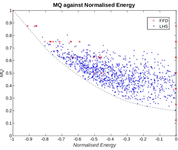
I.7.2.1 Full Factorial Design... 42

I.7.2.2 Latin Hypercube Square ... 43

I.7.2.3 fmincon SQP ... 44

I.7.2.4 Genetic Algorithm (GA) ... 46

I.8SUMMARY ... 47

CHAPTER II – METHODOLOGY AND TOOL DEVELOPMENT ... 48

II.1INTRODUCTION ... 49

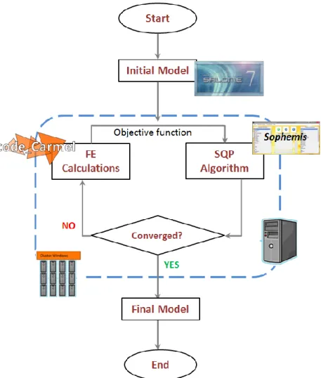
II.2COUPLING OF CODE_CARMEL AND SOPHEMIS ... 49

II.2.1 Overall Process ... 49

II.2.2 Configurations of the Coupling ... 51

1. Local Utilisation ... 51

2. Distant Utilisation ... 51

3. Distant and Distributed Utilisation ... 52

II.3CHOICE OF TOMETHOD –DENSITY METHOD ... 52

Global TO Process with Density Method ... 54

II.4NONLINEAR BEHAVIOUR OF MATERIALS FOR TO USING CODE_CARMEL-SOPHEMIS ... 55

Integrating the Nonlinear Calculation in the TO process ... 57

II.53DELECTROMAGNETIC TEST CASE ... 58

II.6BEHAVIOUR ANALYSIS OF TO USING DESIGN OF EXPERIMENTS ... 60

II.6.1 Cubic_Case_8 ... 60

II.6.2 Design of Experiments ... 62

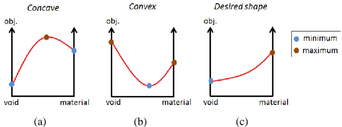
II.6.3 Analysis of the Convexity of the Variables ... 63

vii

II.7.1 Cubic_Case_64 ... 68

II.7.2 Mesh Size Investigation ... 70

II.7.3 Introduction of the Feasibility Factor (FF) in the Methodology ... 72

II.7.4 Using FF in the Optimisation Problem Formulation ... 72

II.7.4.1 FF as Constraint ... 73

II.7.4.2 Proposed Formulation with FF ... 75

II.7.5 Comparison of Proposed Methodology with other Density Mappings ... 78

II.7.6 Comparison with ON/OFF Method ... 83

II.7.7 Repeatability of Solutions ... 84

II.7.8 Using Mesh Elements as Variables ... 84

II.8NONLINEAR BEHAVIOUR OF THE FERROMAGNETIC MATERIALS ... 85

II.9OTHER PROBLEM FORMULATIONS ... 87

II.10SUMMARY AND CONTRIBUTIONS ... 90

CHAPTER III – APPLICATION OF TO METHODOLOGY TO A 3D ELECTROMAGNET ... 91

III.1INTRODUCTION ... 92

III.2STATE OF THE ART ... 92

III.33DFEELECTROMAGNET MODEL ... 95

III.3.1 Finite Element Model ... 95

Optimisation Variables ... 97

III.3.2 Mesh Size Investigation ... 97

Computation of Energy ... 98

Computation of force ... 99

Cross verification with Reluctance Network ... 100

III.4TO OF THE ELECTROMAGNET ... 101

III.4.1 Maximising Energy ... 101

Results ... 102

III.4.2 Maximising Attractive Force ... 103

III.4.2.1 Linear Behaviour of Ferromagnetic Materials ... 104

III.4.2.2 Nonlinear Case ... 109

III.5SUMMARY AND CONTRIBUTIONS ... 115

CHAPTER IV – TO OF A SALIENT POLE SYNCHRONOUS GENERATOR ... 116

IV.1INTRODUCTION ... 117

IV.2STATE OF THE ART ... 117

IV.3SALIENT POLE SYNCHRONOUS GENERATOR (SPSG)MODEL ... 121

IV.3.1 FE Model of the Original SPSG ... 121

viii

IV.4OPTIMISATION OF SPSG... 131

IV.4.1 Recap of TO Process... 131

TO Filter ... 132

IV.4.2 Maximisation of B in the Stator ... 133

IV.4.3 Optimisation of Magnetic Flux Density in Air Gap ... 136

IV.4.3.1 Linear behaviour of Materials ... 137

Example 1 – Average Convergence with Relevant Topology ... 139

Example 2 – Good Convergence with Poor Topology ... 141

IV.4.3.2 Nonlinear Behaviour of Materials ... 143

IV.5SUMMARY AND CONTRIBUTIONS ... 146

CONCLUSION ... 147

SUMMARY AND CONTRIBUTIONS ... 148

PERSPECTIVES ... 149 Methodology ... 149 Tool ... 149 Applications ... 149 REFERENCES ... 151 APPENDICES ... 0 -APPENDIX A ... -1

Calculation of LHS with Sophemis ... 1

-APPENDIX B ... -3

Example of Sophemis Model on Matlab for TO ... 3

-APPENDIX C ... -5

Example of Sophemis windows ... 5

Sophemis window ... 5

Optimisation of a model ... 5

Live visualisation of evolution of iterations ... 6

-APPENDIX D ... -7

Example of files where force is extracted ... 7

Example of file where B is extracted ... 7

-APPENDIX E ... -8

Example of server showing running of code_CarmelSophemis coupling ... 8

-APPENDIX F... -9

Different mesh sizes for 3D FE electromagnet model ... 9

Energy obtained using A and Ω formulations with 3.0 A/mm² ... 9

-ix

Introduction ... I Etat de l’Art ... II Développement de Méthodologie et Outils OT ... III Application à un Electroaimant ... V Application à une Génératrice Synchrone à Pôles Saillants (GSPS) ... VI Conclusion and Perspectives ... VII

x

Figure 1.1 Publications in Electromagnetism from 1992 Till Present [8] ... 6

Figure 1.2 Basic Concept of HM in TO using Square Microcell [11] ... 9

Figure 1.3 Example of Rank-1 and Rank-2 Microstructures [12] ... 10

Figure 1.4 Rectangular Microstructure in 2D and 3D ... 11

Figure 1.5 Plate Optimisation Model and its Microstructure [13] ... 12

Figure 1.6 (a) Hexagonal Microstructure, (b) FE mesh of a Quarter of the Hexagonal Microstructure [10] .. 12

Figure 1.7 Rank Layered Bi-material Microstructures [10] ... 13

Figure 1.8 H-shaped Electromagnet (a) Initial Domain; Volume Constraint of (b) 60%, (c) 70% [15] ... 14

Figure 1.9 Example of 2D domain Ω with Density Method ... 15

Figure 1.10 Comparison of Different Interpolation Schemes ... 18

Figure 1.11 Electrostatic Actuator Design (a) Inital Design, (b) Final Design ... 21

Figure 1.12 Blurring Technique (a) Original Structure, (b) Blurred Structure, (c) Topology Selected according to the Volume Fraction of 0.5 [42] ... 22

Figure 1.13 Contour Representation when a Surface Intersects a Plane [59] ... 24

Figure 1.14 (a) Contour at Zero Level Set, (b)-(d) Evolution of a Contour by Splitting [60] ... 24

Figure 1.15 Representation of Domain Ω and Boundary ... 25

Figure 1.16 Optimised Shape and Flux Distribution (a) ON/OFF (b) Level-set Method [70] ... 27

Figure 1.17 Checkerboard Patterns with (a) Structural Design, (b) Electromagnetic Design ... 29

Figure 1.18 Example of Mesh Dependency of the TO Design [9] ... 29

Figure 1.19 Subgroups of Maxwell’s Equations ... 33

Figure 1.20 Schema of Electromagnetic Domain ... 36

Figure 1.21 B(H) Curve using Marrocco Equation ... 40

Figure 1.22 Latin square Example ... 43

Figure 2.1 Flowchart for Overall TO Process ... 50

Figure 2.2 Local Utilisation Layout ... 51

Figure 2.3 Distant Utilisation Layout ... 52

Figure 2.4 Distant and Distributed Utilisation Layout ... 52

Figure 2.5 (a) Example of Initial Domain, (b) Colour Legend for ρ and µr ... 54

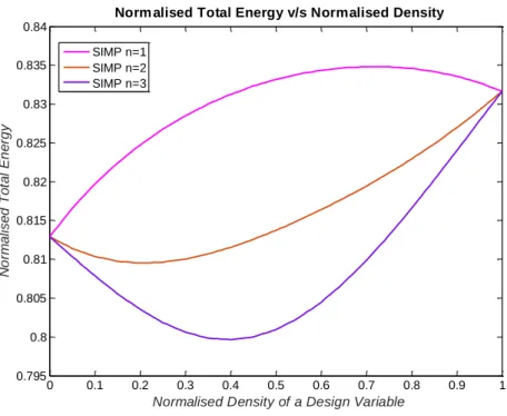
Figure 2.6 Polynomial Mapping for different Penalisation Coefficients n ... 54

Figure 2.7 Block Diagram of TO Process with Polynomial Mapping ... 55

Figure 2.8 µ(H) Curve ... 56

Figure 2.9 H(B) Curve ... 57

Figure 2.10 Block Diagram to Highlight Main Differences using Nonlinear Materials ... 58

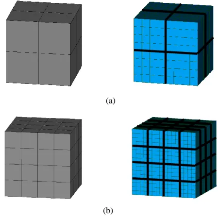
Figure 2.11 Test Cases with respective number of variables (a) 8, (b) 64 ... 59

Figure 2.12 Magnetic Potential Difference Applied to Nodes ... 59

Figure 2.13 Cubic_Case_8 (a) showing 8 zones (variables), (b) showing MPD ... 61

xi

Figure 2.15 (a) Concave, (b) Convex, (c) Desired Shape ... 64

Figure 2.16 Initial Structure with one zone varying ... 65

Figure 2.17 Energy v/s Density for each zone varied ... 65

Figure 2.18 Initial Structure for Two Zones Varied ... 66

Figure 2.19 Energy v/s Density for Two Zones Varied ... 67

Figure 2.20 Example of Continuation Method ... 68

Figure 2.21 Cubic_Case_64 (a) FE Model, (b) Model showing only zones ... 69

Figure 2.22 Magnetic Flux Density Distribution for Maximum Energy (Linear Case) ... 69

Figure 2.23 True Energy v/s Mesh Size of Cubic_Case_64 ... 70

Figure 2.24 Feasibility Factor (FF) w.r.t ρi ... 72

Figure 2.25 Example of biased solution with FF as constraint ... 73

Figure 2.26 Evolution of (a) Energy, (b) MQ, (c) FF w.r.t the Number of Evaluations ... 74

Figure 2.27 Energy and FF against Weightage Coefficient λ... 76

Figure 2.28 (a) Final Topology, (b) Energy, (c) FF, (d) MQ, (e) Sum of Objectives ... 78

Figure 2.29 Comparison of Density Methods with Proposed Methodology for (a) Energy, (b) MQ, (c) FF, against the Number of Evaluations ... 80

Figure 2.30 Magnetic Flux Density Distribution for Topology with Proposed Methodology (Linear Case) ... 81

Figure 2.31 Effect of Initial Points on Optimal Results ... 84

Figure 2.32 Model using Mesh Element as Variable with (a) Geometry, (b) FE Model ... 85

Figure 2.33 Magnetic Flux Density Distribution with Maximum Energy (Nonlinear Case) ... 86

Figure 2.34 Magnetic Flux Density Distribution of Optimal Topology (Nonlinear Case) ... 87

Figure 2.35 Magnetic Flux Distribution with MPD=15 AT (a) Linear Case, (b) Nonlinear Case ... 89

Figure 3.1 (a) H-Shaped Electromagnet, (b) Design Domain, Optimised Shape with Volume Constraint(c) 60%, (d) 70% [15] ... 93

Figure 3.2 (a) C-core Actuator, (b) Initial Domain, Results in (c) Linear Case, (d) Nonlinear Case [18] ... 94

Figure 3.3(a) Initial Domain, (b) Density Method Results (coarse mesh on left & fine on right), (c) LSM (conventional on left and advanced on right) [64] ... 94

Figure 3.4 TO of Magnetic Yoke (a) Design Domain, (b) Optimised Yoke shape, (c) Magnetic Flux Line Plot ... 95

Figure 3.5 (a) Electromagnet Model with Dimensions, (b) Quarter Model, (c) Model with Boundary Conditions ... 96

Figure 3.6 Energy for Different Mesh Sizes ... 98

Figure 3.7 Nodes on which Force is Calculated ... 99

Figure 3.8 Attractive Force v/s Number of Nodes ... 100

Figure 3.9 Reluctance Network for Electromagnet ... 101

Figure 3.10 Case of Maximum Energy in the Electromagnet for Linear Material Behaviour ... 102

Figure 3.11 Optimal Topology while Maximising Energy with MQ = 0.8 ... 103

Figure 3.12 (a) β=0.8, (b) β=0.6, (c) β=0.4, (d) β=0.2 ... 104

xii

Figure 3.14 Convergence Graphs for Linear Case with 𝜷 = 𝟎. 𝟐 ... 108

Figure 3.15 Position of Non-converged Variables ... 109

Figure 3.16 Magnetic Flux Density Distribution in Nonlinear Case with Variables as Iron ... 110

Figure 3.17 Marrocco Saturation Curve ... 110

Figure 3.18 (a) β=0.8, (b) β=0.6, (c) β=0.4, (d) β=0.2 ... 111

Figure 3.19 Nonlinear Case𝜷 = 𝟎. 𝟐 (a) Overall Objective, (b) Force, (c) FF, (d) MQ, (e) Density of Variables ... 114

Figure 4.1(a) Design Region of Machine, (b) Cell Division for TO, (c) Final Results ... 118

Figure 4.2 (a) Initial IPM Motor, (b) TO Domain in Red, (c) Material Removed in the Optimisation process (Green), (d) Optimised Shape, (e) Optimised Radial Component ... 119

Figure 4.3 (a) Initial Domain of IPM, (b) Optimised Topology... 120

Figure 4.4 (a)&(b) Initial Design Space and Positions, Optimised Topologies for (c) 5 Iterations (d) 8 Iterations ... 121

Figure 4.5 SPSG (a) Geometry, (b) Mesh ... 123

Figure 4.6 Spatial Distribution of B in the Machine with (a) Linear, (b) Nonlinear Material Behaviour ... 125

Figure 4.7 Magnetic Flux Density in Air Gap with (a) Linear, (b) Nonlinear Material Behaviour ... 126

Figure 4.8 Domain to be Optimised (a) FE model, (b) Zoom, (c) Geometry ... 128

Figure 4.9 Spatial Distribution of B in the Machine for (a) Linear, (b) Nonlinear Behaviour of Materials ... 129

Figure 4.10 Magnetic Flux Density in Air Gap for (a) Linear, (b) Nonlinear Behaviour of Materials ... 130

Figure 4.11 Block Diagram for Overall TO Process ... 131

Figure 4.12 Zones Numbering ... 132

Figure 4.13 (a) Topology Before Filter, (b) ρsum for each zone, (c) Filtered topology with 𝒗 = 𝟎. 𝟎𝟓 and 𝒘 = 𝟎. 𝟗𝟓, (d) Filtered Topology with 𝒗 = 𝟎. 𝟏 and 𝒘 = 𝟎. 𝟗 ... 133

Figure 4.14 Maximisation of B in the Stator Yoke ... 134

Figure 4.15 Topologies in (a) Linear, (b) Nonlinear, B Distribution in (c) Linear, (d) Nonlinear ... 135

Figure 4.16 Modulus of Sine Curve Imposed ... 136

Figure 4.17 (a) Spatial Points, (b) Convergence of Objective ... 138

Figure 4.18 Unfiltered Resuts (a) Topology, (b) B Distribution, (c) B in Air Gap ... 138

Figure 4.19 Filtered Results (a) Topology, (b) B Distribution, (c) B in Air Gap ... 139

Figure 4.20 (a) Spatial Points, (b) Convergence of Objective ... 140

Figure 4.21 Unfiltered Resuts (a) Topology, (b) B Distribution, (c) B in Air Gap ... 140

Figure 4.22 Filtered Resuts (a) Topology, (b) B Distribution, (c) B in Air Gap ... 141

Figure 4.23 For 13 Spatial Points (a) B in Stator and in Rotor Used in Constraint (b) Objective Convergence, (c) B in Air Gap with 13 points, (d) B in Air Gap with 73 points, (e) Optimal Topology ... 142

Figure 4.24 (a) Convergence of Objective, (b) B in the Air Gap, (c) Unfiltered Topology, (d) B Distribution ... 143

xiii

List of Tables

Table 1.1 Recap of the Interpolation Schemes ... 18

Table 1.2 Combinations for Final Material ... 19

Table 1.3 Example of Full Factorial Design ... 43

Table 1.4 Latin Square Experimental design ... 44

Table 1.5 Recap of Tool Chosen ... 47

Table 2.1 Recap of Mesh Size Investigation Information ... 71

Table 2.2 Biased Solution’s Information ... 73

Table 2.3 Comparison of Different Mappings with Proposed Method ... 82

Table 2.4 Results with GA ... 83

Table 2.5 Results with Nonlinear Behaviour of Materials ... 86

Table 2.6 Comparison of Linear and Nonlinear Cases... 88

Table 3.1 Information about the TO Results with Energy ... 103

Table 3.2 Additional Information about the TO Results ... 105

Table 3.3 Additional Information for Nonlinear Case ... 112

xiv

List of Abbreviations

Abbreviation Full Form

BLDC Brushless DC Motor

DoE Design of Experiments

FE Finite Element

FF Feasibility Factor

FFD Full Factorial Design

GA Genetic Algorithm

HM Homogenisation Method

IPM Interior Permanent Magnet

LHS Latin Hypercube Square

LSM Level-Set Method

MPD Magnetic Potential Difference

MQ Material Quantity

RAMP Rational Approximation of Material Properties

RN Reluctance Network

SIMP Solid Isotropic Material with Penalisation

SPSG Salient Pole Synchronous Generator

SQP Sequential Quadratic Programming

1

We are currently living in a very demanding era, pushing the human intelligence towards the invention of more effective technologies and the improvement of existing ones in the pursuit of optimality, if not excellence. We, research scientists, are the most active players in this quest for superiority. With the help of other technologies such as computers, which have now become ineluctable tools, we are capable of engaging into more tedious calculations and simulations, drawing us closer to our goals. This has brought a big boost in engineering in general, including the electrical field which is our main concern.

The electrical engineering laboratory (Laboratoire d’Électrotechnique et d’Électronique de Puissance, L2EP), within which this thesis was carried out, has many ongoing works on the optimisation of electromagnetic devices, such as electrical machines, amongst others. This thesis was therefore oriented towards this same mind-set. Optimisation of machines, for example, is a vast subject which can extend from the optimisation of one simple parameter to the whole machine. Classically, engineers start off from already existing structures and optimise some dimensions to yield a better design. But in doing so, the optimisers always find themselves constrained by the initial shape of the structure, and thus reduces the degree of freedom. Moreover, in a constant search of new structures, we are very often biased by existing ones which can obstruct our sense of innovation. For this reason, we will use a different approach to this type of problem: the Topology Optimisation (TO).

TO is an original way of finding new designs of structures without having any layout a priori on the latter. This infers that the optimisation problem is defined in such a way that the existing structures are not considered in the problem, but the TO process is rather free to find the optimal structure it judges the best, according to the information specified. Scientific researchers in the mechanical/structural field are the pioneers in TO, and have taken many decades before coming up with such a methodology. The results were so interesting that they attracted researchers from various other fields, including electromagnetism.

TO remains till date amongst the most complex forms of optimisation as it requires equal expertise in optimisation algorithms, as well as numerical modelling of structures. In our case, the numerical modelling method used is Finite Element (FE) Analysis. Moreover, depending on the nature of the models, which are electromagnetic in our case, extensive knowledge is also desired in the same field to be able to interpret the results obtained, and hence redirect the works on the right path.

The main aim of this thesis is to develop and acquire the necessary skills and proficiency to be able to optimise the topology of any electromagnetic device, whether simple or complex.

2

To achieve this, a number of stepwise objectives must be enacted to successfully reach our goal.

The first objective is to develop and test a functional tool for TO of electromagnetic devices. The development of the TO tool will be based on the 'home-made' tools available at the L2EP, namely code_Carmel for solving FE numerical models, and Sophemis for solving optimisation problems. A coupling of both will have to be done to create a functional TO tool. To test the latter, it is important to have a simple, yet effective test case to assess its characteristics. For this purpose, an academic 3D test case will have to be developed and parameterised. Its electromagnetic nature should be straightforward and easily understood, and the FE model should also be solved rapidly.

The second objective is to develop a methodology for TO, based on the existing ones such as Density Methods, ON/OFF Methods and so on. The proposed methodology should allow us to overcome the problems usually met with the other methods, for a more effective TO. For a paramount testing of the latter, the academic test case will again be used.

Furthermore, the consideration of the nonlinear behaviour of the ferromagnetic materials is often overlooked in TO due to its tedious setting and high computation time, despite being a very important aspect of electromagnetic modelling. If the electromagnetic device is operating at or near saturation point, and the latter is not considered in the TO process, this might yield incorrect optimal structures. Therefore, the third objective is to adapt the TO tool so that it takes into account the nonlinear behaviour of the materials, and hence allow us to analyse its effects. It will also have to be compared with cases of linear material behaviour to put forward its importance. A 3D electromagnet will be used for this purpose as it represents a more real test case, and hence a more judicious appraisal. The FE model of the electromagnet will also have to be developed and parameterised.

Last but not least, the fourth objective of this thesis work is to apply the developed tools and methodology to a more complex, electrical engineering device: a Salient Pole Synchronous Generator (SPSG). It is desired to see the different topologies obtained w.r.t various optimisation problems. The assessment of the process’s behaviour can help us gather enough information to strive towards better solutions in the future.

We will see throughout this manuscript how all these objectives contribute to approach the main aim of this thesis work. The TO process is a complex one, as mentioned before, and should be tackled step by step for productive results. A plan of the work accomplished in the manuscript to guide the reader on the course of the latter is presented here. The manuscript is mainly divided into four chapters:

3

1. Chapter I: A state of the art of the various existing TO methods is done. The method used to complement the proposed methodology of this thesis work is justified. The 'home-made' numerical tools for FE analysis and optimisation are elaborated, as they will further be used to compose the TO tool developed.

2. Chapter II: The development of the TO tool is detailed, as well as the coupling between code_Carmel and Sophemis. A methodology for TO based on the existing methods is proposed. The academic test case is used to test and validate the latter. The consideration of the nonlinear behaviour of the ferromagnetic materials in the TO calculations is developed and explained in this chapter, and tested on the academic test case. Additional investigations are made on various aspects of TO with this model, serving to identify strengths and limitations of the methodology. 3. Chapter III: The TO tool and methodology are used to optimised the topology of the

iron core of the 3D electromagnet. Various cases of optimisation problems will be presented. Calculations for linear and nonlinear behaviour of materials are both done, and the results are compared and analysed.

4. Chapter IV: The TO of the rotor top of the SPSG is done w.r.t different optimisation problems, and the viability of the various topologies are analysed.

We will conclude the manuscript with some opinions and assertions we have built up on TO during this thesis work, and with some interesting perspectives for future works on the topic.

4

5

I.1 Introduction

TO has sparked a sudden interest amongst researchers in the past two decades, owing to its originality and ability to produce innovative designs. Before heading to any kind of computation, it is interesting to step into the history of TO to understand its evolution, and the methods associated with it.

The first segment of this chapter is dedicated to the history of Topology Optimisation (TO) over time, and how the different methods evolved till present day. Some TO methods were developed from existing ones, while others were established from popular optimisation methods initially designed for different purposes in other fields. Firstly, the main TO methods shall be introduced without focusing on the field for which it was conceived, whether mechanical, electrical and so on. Afterwards, the main applications w.r.t electrical engineering will be evoked with some examples and findings.

In the second segment, the numerical tools used to carry out the TO process are encompassed. This englobes the classical Finite Element (FE) methods and algorithms mainly used for the purpose of modelling and optimisation. Both tools used are developed at the L2EP within the OMN (Outils et Méthodes Numériques) team. TO normally requires the use of both tools coupled together, but this section will focus on them individually as the coupling is a significant part developed during this PhD work, and hence to be presented in the next chapter.

Finally, the conclusion will hint at the methods retained for the rest of this thesis work, and briefly uncover the content of the following chapter.

I.2 Origin of the Topology Optimisation Idea

The desire to generate optimal structures dates a long way back when numerical tools did not even exist. Works were already being carried out in the mechanical field to find the limits of reducing the amount of material present in frame structures without degrading the former’s tensile stress and strain.

In 1904, Michell [1] proposed a mathematical study to sustain given forces in structures attaining the limits of economy of material. The idea was definitely in a TO mind-set, but was

left unexploited for many decades before Rozvany [2] published his work on the optimisation

of perfectly plastic and elastic grillages of maximum stress and stiffness with minimum weight solutions . But as for the previous case, the study was essentially a mathematical formulation without practical applications. Later in 1972, Rozvany and Prager [3] studied the

6

minimum weight design of grillage of perfectly plastic beams that are on the verge of plastic collapse under given loads. They proposed a discretisation of the beams constituting the grillage, but the study was mostly based on changing the number of discretisation, and hence beams. The idea of discretising the optimisation domain was hence introduced.

In 1988, Bendsøe and Kikuchi [4] innovated with the Homogenisation Method (HM) applied to a generalised mechanical TO problem, revolutionising the subject and inspiring the sheer interest of other authors. Afterwards, Bendsøe introduced the Direct approach [5] based on the HM, but easier in application, and therefore more engineer-oriented. The idea was further elaborated in [6] where the authors adapted the Direct Method into SIMP (Solid Isotropic Material with Penalisation) Method for intermediate densities, which will be detailed in the future sections. But it wasn’t until 1996 that TO was introduced in the electromagnetism community by Dyck and Lowther [7], presenting the OMD (Optimised Material Distribution) Method.

According to Scopus [8], various fields such as mechanics, electromagnetism, computer science, physics and astronomy, energy, chemistry, neuroscience and econometrics use TO, amounting to some 3600 publications since 1986. The number of papers on TO in electromagnetism holds a fair share as shown in Figure 1.1, for year 1992 till present. This includes conference and journal papers, and we can see a steep rise from around 2007. As for the leading countries in TO in electromagnetism, Scopus surveys the greater number of works from Japan, USA, China and South Korea.

Figure 1.1 Publications in Electromagnetism from 1992 Till Present [8]

The state of the art in the next sections will focus on the TO methods in electromagnetism, but also a few in mechanical since the methods for the former were actually derived from the latter. Despite not having the same way of formulating the problem, they are closely related. The next section will concisely enumerate the main differences between TO in mechanical

7

and electromagnetism to justify why the methods cannot be directly translated from one to the other.

I.3 Differences between Mechanical and Electromagnetic Structures

Regarding TO, the main dissimilarity is that in mechanical structures, it is often desired to have lighter designs while respecting the given mechanical constraints like tensile stress and strain, whereas in electromagnetic structures, it is rather required to have magnetically optimal structures w.r.t the magnetic force, magnetic flux density, EMF and so on.

Another essential difference is that in electromagnetism, the nonlinearity of the ferromagnetic materials constituting the majority of the devices must be taken into account. Since we are dealing with the permeability of materials, we must take into account the saturation effect. This implies a limitation of the material to allow flow of more magnetic flux at some point due to their saturation. After this point, there is also a change in the material’s behaviour. These effects do not have to be considered in mechanical structures, but can be a turning point in electromagnetism.

We can also evoke the importance of the movement of electromagnetic devices such as in motors and generators to produce the expected output, while in mechanical devices such as beams, bridges, frames or housings, they are usually required to be stationary and withstand the prescribed load.

The above factors alone represent a substantial hindrance to TO as they largely increase the computation time for the resolution of the models. Computation time usually varies from model to model, and can take several hours to several days. It could be a good practice to keep a step-wise procedure of finding the optimal topology of electromagnetic structures by gradually increasing the difficulty. For instance, a TO using linear materials is usually the stepping stone due to its relative rapidity. Once the correct problem formulation is found, and the solution obtained corresponds to a suitable one, a TO using nonlinear materials can afterwards be envisaged. Subsequently, if the electromagnetic device involves movements (such as in electric machines), the latter can also be added to the TO calculations for a closer consideration of real conditions.

Before getting into these details, it is fair to first introduce the various existing TO methods to later narrow down our choice for this work.

8

I.4 Topology Optimisation Methods

Since the introduction of TO, various authors have proposed diverse methods of tackling the problem. This section reviews the most popular methods in literature. The Homogenisation Method (HM) is covered first, introducing its different variants. Thereafter, the Density Method is presented and its clear relation with the HM is evoked. Subsequently, the ON/OFF Method is discussed, and its link with the Density Method is also explained. Last but not least, the Level-set Method is outlined to see its completely different background when compared to the first 3 methods. For each method, the algorithms used for optimisation, and the applications in electromagnetism are shortly illustrated to provide a wider overview of what has been done in literature.

I.4.1 Homogenisation Method (HM)

HM was one of the first and most pioneering TO methods introduced in literature by Bendsøe and Kikuchi [4]. It was basically developed for mechanical/structural designs with the aim of reducing material constituting the structures for lighter and stronger ones. It deals essentially with anisotropic/ composite materials, with an interpolation between void and full material. It was founded on theoretical work that proved the existence of solutions could be resolved by modifying the design space to include relaxed designs, for instance in the form of composites [9]. These design spaces made of composites can be modelled by materials with microstructures, and it exists in different types such as rotated, layered or rectangular microstructures amongst others. Hence, this involves the consideration of other parameters such as orientation and dimensions of each microstructure. In a TO problem, each microstructure would normally represent a variable to be optimised, and therefore we have more than one parameter for each variable depending on the microstructure type. The optimal design of structures is closely connected with the study of microstructures and finding the effective homogenised material properties for composite microstructures [4]. The following section reviews some of the existing microstructures.

I.4.1.1 One-Material Microstructures

In one-material microstructures, the material model contains one material with one or more voids. If a portion (or percentage) of a region is made of voids, material is not placed there. Otherwise, if there is no porosity in an area, material is placed in that area [10]. An example is given in Figure 1.2 to show the basic concept of HM in TO using a square microcell with centrally placed rectangular hole as the material model. The top of the figure shows the

9

domain before optimisation, and the bottom, after optimisation. The black area represents material, the white represents void, and the grey area represents intermediate materials. This means that the material found these types of regions is neither fully solid nor void, but is instead consists of a certain percentage of solid and void. This makes it an intermediate material which is not manufacturing-friendly, and hence usually undesired in the final solution. We will go deeper into this matter throughout this thesis work.

Figure 1.2 Basic Concept of HM in TO using Square Microcell [11]

Various one-material microstructures exist, and some are presented below. They can also directly be implemented into a FE code to be used as main elements of the domain. For instance, instead of using tetrahedral elements, which is the most common practice, it could also be interesting to use the one-material microstructures, and the different parameters of each microstructure would represent the variables of the optimisation problem.

Rank Layered Microstructure

The basic idea of this category is to find extremal microstructures with maximum rigidity (or equivalent minimum compliance). A layered microstructure of rank-p can be used, with p ranging from 1 and above, but usually ranks 1 and 2 are used for simplicity. Usually, in a rank-p, there are alternating layers of void and solid material, with layers of the ranks being orthogonal to each other. For example, in rank-1 material, there are only alternating layers of solid material and void in one direction. In rank-2 material, in addition to the initial alternating layers, there are orthogonal alternating layers of solid material. Figure 1.3 illustrates a rank-1 and rank-2 layered microstructure.

10

Figure 1.3 Example of Rank-1 and Rank-2 Microstructures [12]

In TO, rank-2 layers are most commonly used. In this case, the elements of the matrix of elasticity coefficients are functions of 3 parameters: γ, ϑ and θ (as in Figure 1.3), where ϑ and γ lie between 0 and 1, limits included. The parameter γ represents the width of the layers in rank-1 material, while ϑ represents the width of the orthogonal layer in a rank-2 material. The

parameter θ gives the orientation of the layers. The volume Ωs occupied by the solid is given

in (I-1):

𝛺𝑠 = ∫ (𝜗 + 𝛾 − 𝜗𝛾)𝑑𝛺

𝛺

(I-1)

and the density of the composite can be written as in (I-2):

𝜌 = 𝜌(𝜗, 𝛾) = (𝜗 + 𝛾 − 𝜗𝛾)𝜌_𝑠 (I-2)

where ρs is the density of the solid [12]. It must be noted that it is possible to vary the cell

relative density from 0 to 1 by changing the value of ϑ and γ.

The advantage of rank layered material is that the effective material properties can be derived analytically. The main weakness is that the material cells do not provide resistance to shear stress in between layers.

Rectangular Microstructure

In this category, the microstructure is a square cell with a centrally placed rectangular hole in 2D, whereas in 3D, it is represented by a cubic cell with a rectangular parallelepiped hole, as in Figure 1.4.

11

Figure 1.4 Rectangular Microstructure in 2D and 3D

Rectangular microstructure is one of the most commonly used for TO with HM. The area

Ωc is occupied by the solid material in the base cell as given in (I-3), and the volume Ωs is

occupied by the solid material in the design domain as given in (I-4).

𝛺_𝑐 = 1 − 𝑥_𝑎. 𝑥_𝑏 (I-3)

𝛺𝑠 = ∫ (1 − 𝑥𝑎. 𝑥𝑏)𝑑𝛺 𝛺

(I-4)

where xa and xb lie between 0 and 1, limits included. The angle of orientation is also θ. For

different orientations, the properties of elastic constitutive matrix are changed.

The main strength of rectangular microstructures making it popular in TO with HM is due to the smaller number of variables required if a square void is chosen. The main drawbacks are that, on one side the homogenisation equation has to be solved by numerical techniques, and on the other side the optimisation results often contain intermediate regions.

Triangular Microstructure

Not very popular in TO, the triangular microstructure is a very complicated one, making it more tedious in numerical implementation and hence increasing computational cost. An example of the plate model setup for triangular microstructure is given in Figure 1.5. The main strength is that the true strain energy can be calculated numerically, which is not always the case with the other microstructures.

12

Figure 1.5 Plate Optimisation Model and its Microstructure [13] Hexagon Microstructure

Initially presented in [12], this type of microstructure is also called honeycomb based cell and is given in Figure 1.6(a), along with the dimensions. They have the same advantage and disadvantage as the triangular microstructure. Figure 1.6(b) depicts a FE mesh for a quarter of the honeycomb cell.

Figure 1.6 (a) Hexagonal Microstructure, (b) FE mesh of a Quarter of the Hexagonal Microstructure [10]

I.4.1.2 Bi-material Microstructure

Bi-material microcells involve two solid materials, whether voids are included or not. The geometry parameters of the hard materials, soft materials and voids are set as the design variables of the optimisation problem. As for the one-material microstructure, if a region consists of voids only, material is not placed there. Likewise, if a region has no porosity (no voids), a solid material is placed there. Rank layered microstructures are most commonly used for bi-material microstructures [10]. Figure 1.7 shows examples of bi-material microcell with rank layered microstructures. The black and blue areas represent different solid materials, while the white area represents void. In the case of Figure 1.7(a), optimisation is done only between two solids. The variables shown in the figure are allowed to vary between 0 and 1, limits included. The effective material properties can be derived analytically, and the method can be applied to both 2D and 3D models.

13

Figure 1.7 Rank Layered Bi-material Microstructures [10]

The volumes occupied by solid material Ω1 (black) and solid material Ω2 (blue) are given in

(I-5) and (I-6) respectively [12].

𝛺𝑠 = ∫ (𝜗 + (1 − 𝜗). 𝛾1. 𝛾2)𝑑𝛺 𝛺 (I-5) 𝛺𝑠 = ∫ ((1 − 𝜗). (1 − 𝛾1). 𝛾2)𝑑𝛺 𝛺 (I-6)

Despite the numerous ways of formulating the optimisation domain using HM, it remains more popular in the mechanical field than in electromagnetism. The main reason would be the relative complexity of defining an optimisation problem with HM because of the various variables needed for one microstructure. Other methods, more adapted to electromagnetism were developed from HM, and will be seen in the later sections.

I.4.1.3 Optimisation Algorithms used with HM

Due to the high dimension of the optimisation problem using HM as described above with multiple variables per cell, it narrows the choice for algorithm classes. Most works with HM apply sensitivity-based approaches using analytical derivatives calculated directly from the definition of the homogenisation problem [14]. Amongst the popular algorithms are the Sequential Linear Programming (SLP), Method of Moving Asymptotes (MMA) or a variety of iterative update rules based on explicit optimality conditions.

I.4.1.4 Applications of HM to Electromagnetic Problems

The HM, being primarily derived for mechanical/structural designs has mostly been applied to the topology optimisation of cantilever beams, bridges and trusses. Its application to electromagnetic problems is quite rare and remains much dreaded due to the large number of variables. One of the few works that has been presented on TO using HM is [15], where the authors determine the optimal material distribution in a design domain .by changing the inner

(b)

14

hole size and rotational angle of the unit cell. The objective is to maximise the magnetic mean compliance of an H-shaped magnet, which is the same as maximising the magnetic vector potential, and therefore improving the electromagnet performances, according to the authors. Different volume constraints are applied to the design domain to see the behaviour, and the materials used are assumed to be linear. Examples of the topologies obtained are given in Figure 1.8.

Figure 1.8 H-shaped Electromagnet (a) Initial Domain; Volume Constraint of (b) 60%, (c) 70% [15]

I.4.2 Density-based Methods

Derived from the HM, the Density-based Method was elaborated to overcome some difficulties with the former. Firstly, the generation of areas with porosity were not quite desirable, due to their problematic tendency for manufacturing. An example of porosity would be during the use of rectangular microstructures in HM (Figure 1.2), where the cell would not completely be made of solid material or void. In the advent of many such microcells occurring adjacently, this would form a porous structure, which would be challenging to homogenise for any manufacturing purpose. Another issue could be the need for various design variables for one microcell. Since the process of topology optimisation is already known to be a long one, this would only add up to the lengthy calculation time. For instance, if the rectangular microstructure is again considered, there are 3 design variables in 2D

namely xa, xb and θ, while there are additional ones in 3D. Regarding practicability, the HM is

also known to be tedious in implementation, whether for mechanical or electromagnetic problems. To limit the aforementioned difficulties, the Density Method was introduced. It must be pointed out that Direct Approach, Engineer’s Method or SIMP Method are the different names given to Density Method.

In [5], the Direct Approach was initiated and tested on a mechanical support structure. An artificial density function ρi was introduced, with 0 ≤ 𝜌𝑖 ≤ 1, and used to calculate the Young’s Modulus E of cell i as in (I-7). The Young’s Modulus of the solid material is given by E', the penalisation coefficient by n, and i is an element of optimisation domain Ω. Figure 1.9 depicts a typical 2D domain used in Density Method.

15 𝐸_𝑖 = |𝜌_𝑖|𝑛_{. 𝐸}

𝑖′ (I-7)

Figure 1.9 Example of 2D domain Ω with Density Method

The artificial density values of ρi lying between 0 and 1 essentially represent a proportion of

solid material or void. Of course, it is desired to have either solid material (ρ=1), or void (ρ=0) as final material in the cell, instead of having intermediates unless they are defined in the library of materials of the optimisation problem. The main interest here is that the material properties between the solid and void are interpolated with a smooth continuous function which depends on the material density ρ. The penalisation coefficient n is used to change the interpolation behaviour with n ≥ 1, and actually apply a ‘penalty’ on the design variable ρ to transform it to either solid material or void. This part will be detailed in the following sections. The term SIMP (Solid Isotropic Material with Penalisation) was adopted in [16] by Rozvany et al. to refer to this same method and is today the most commonly used in literature. But the equation relating the various above mentioned parameters can differ in nature. Throughout time, many of these equations or so-called Interpolation Schemes have been introduced in literature, and the main ones are presented in the next section. All the equations will be given in terms of relative permeability.

I.4.2.1 Interpolation Schemes

In [7], the Direct Method is revisited for application in the electromagnetic field. The authors propose a new philosophy of considering the method as a distribution of material in space, and called it OMD (Optimised Material Distribution). This point of view is still used today, as it is a more practical way of establishing the problem. In a domain to be optimised,

ρi = 1 _{ρi = 0}

0 < ρi < 1 Domain Ω

16

the material properties are defined at every point in space. Hence, for efficient distribution, the domain has to be discretised into cells. For magnetic devices, parameters such as permeability, permittivity and conductivity are used to represent the materials, where each cell can take these characteristics. For an optimisation, it is possible to consider many properties at the same time, or one at a time. The most common case is to consider only permeability as the material properties, as it is usually desired to optimise the topology of ferromagnetic materials. The relationship between the material density and the permeability was very much inspired from (I-7) and is given in (I-8), dubbed as Geometric Mapping in [7]. The main difference is that in the latter, the density is used as a power so that the minimum relative permeability (air) is always 1.

𝜇𝑟_𝑖 = 𝜇𝑟_𝑎𝑖𝑟𝜇𝑟_{𝑖𝑟𝑜𝑛}𝜌𝑖 _(I-8)

The relative permeability and material density in cell i are given by µri and ρi respectively,

and the relative permeability of free space and the solid material are given by µrair and µriron

correspondingly. Following this work, other authors proposed different interpolation schemes

between µri and ρi. For example in [17] and [18], the Polynomial Mapping is introduced, as

given in (I-9), and is clearly inspired from (I-7) and (I-8):

𝜇𝑟𝑖 = 𝜇𝑟𝑎𝑖𝑟+ (𝜇𝑟𝑖𝑟𝑜𝑛− 𝜇𝑟𝑎𝑖𝑟)𝜌𝑖𝑛 (I-9)

where 0 ≤ 𝜌_𝑖 ≤ 1 and 𝑛 ≥ 1. For 𝑛 = 1, the function is a linear one, and normally referred

to as Permeability Mapping in literature. The higher the value of n, the greater will be the variation of the gradient of the curve. This actually helps in the ‘penalisation’ of the intermediate density values to 0 and 1. The authors in [17] test the mapping using permittivity of a dielectric material instead of permeability, to be consistent with the nature of their problem. In [18], the authors test the interpolation scheme by optimising an electromagnet.

In [19] and [20], the authors initially propose an interpolation scheme with the inverse of

the Young’s Modulus E, as given in (I-10), for ith

cell. In [9], the authors revisit the function and illustrate it as a Rational Function, or RAMP (Rational Approximation of Material Properties), as it might have been named in other circumstances. The RAMP Function is given in (I-11). 1 𝐸_𝑖 = 1 𝐸_𝑚𝑖𝑛+ 𝜌𝑖( 1 𝐸₀ − 1 𝐸_𝑚𝑖𝑛) (I-10)

17 𝐸𝑖 = 𝐸𝑚𝑖𝑛+

𝜌_𝑖

1 + 𝑞(1 − 𝜌_𝑖)(𝐸0 − 𝐸𝑚𝑖𝑛) (I-11)

Of course, the function can also be adapted to electromagnetics by using permeability

instead of Young’s Modulus, as in (I-12). Usually 𝑞 ≥ 0, but the authors suggest that if Emin is

much smaller than E0, then it is wise to use a very large of q so that the final design is free of

intermediate densities. It must be noted that, if 𝑞 = 0, the interpolation scheme is linear. 𝜇𝑟𝑖 = 𝜇𝑟𝑎𝑖𝑟+

𝜌𝑖

1 + 𝑞(1 − 𝜌𝑖)(𝜇𝑟𝑖𝑟𝑜𝑛− 𝜇𝑟𝑎𝑖𝑟) (I-12)

In [21], the authors proposed the use of reluctivity instead of permeability, hence the

Reluctivity Mapping as in (I-13). The topology optimisation of an electromagnet is treated in

the same paper using this mapping. The resulting permeability when the cell i take the properties of iron or air should be the same when using reluctivity in the equation, except that the shape of the curve for intermediate materials (between 0 and 1) will be different. This is depicted in the next section.

𝜇𝑟_𝑖 = ₁ 1

𝜇𝑟_𝑎𝑖𝑟 + (𝜇𝑟1_{𝑖𝑟𝑜𝑛}−𝜇𝑟1_𝑎𝑖𝑟) 𝜌𝑖

(I-13)

In [22], the authors propose mathematical sequences as interpolation schemes where the

Uniform Sequence, Geometric Sequence and Arithmetic-geometric Sequence are evoked.

An example of the Uniform Sequence adapted to the permeability is given (I-14).

𝜇𝑟_𝑖 = 𝜇𝑟_𝑎𝑖𝑟+ (𝜇𝑟𝑖𝑟𝑜𝑛− 𝜇𝑟𝑎𝑖𝑟

𝑚 ) ∑ 𝜌𝑖𝑘

𝑚

𝑘=1

, ∀𝜌 ∈ [0,1] (I-14)

The value of m can be varied according to the order of the summation terms desired.

Table 1.1 recaps the different interpolation schemes and Figure 1.10 illustrates the curves obtained with each, for 𝜇𝑟𝑎𝑖𝑟 = 1, and 𝜇𝑟𝑖𝑟𝑜𝑛 = 2000. The next chapter will compare their efficiency with an academic test case.

18

Table 1.1 Recap of the Interpolation Schemes

Interpolation Scheme Equation Penalty Coefficient Polynomial 𝜇𝑟_𝑖 = 𝜇𝑟_𝑎𝑖𝑟 + (𝜇𝑟_{𝑖𝑟𝑜𝑛}− 𝜇𝑟_𝑎𝑖𝑟)𝜌_𝑖𝑛 n Geometric 𝜇𝑟_𝑖 = 𝜇𝑟_𝑎𝑖𝑟𝜇𝑟_{𝑖𝑟𝑜𝑛}𝜌𝑖 _- Reluctivity 𝜇𝑟_𝑖 = ₁ 1 𝜇𝑟𝑎𝑖𝑟+ ( 1 𝜇𝑟𝑖𝑟𝑜𝑛− 1 𝜇𝑟𝑎𝑖𝑟) 𝜌𝑖 - RAMP _𝜇𝑟 𝑖 = 𝜇𝑟𝑎𝑖𝑟+ 𝜌𝑖 1 + 𝑞(1 − 𝜌_𝑖)(𝜇𝑟𝑖𝑟𝑜𝑛− 𝜇𝑟𝑎𝑖𝑟) q Uniform Sequence 𝜇𝑟_𝑖 = 𝜇𝑟_𝑎𝑖𝑟+ (𝜇𝑟𝑖𝑟𝑜𝑛− 𝜇𝑟𝑎𝑖𝑟 𝑚 ) ∑ 𝜌𝑖𝑘 𝑚 𝑘=1 𝑤ℎ𝑒𝑟𝑒 ∀𝜌_𝑖 ∈ [0,1] m

Figure 1.10 Comparison of Different Interpolation Schemes

, ρi

19

These mapping equations represent a way of linking the artificial density ρi (variable) to the

property of the cell i by showing their evolution over the range of ρi. These mappings are

useful during optimisation as the density ρ is taken as variable instead of the permeability. Given the smaller range of 0 ≤ 𝜌𝑖 ≤ 1, it renders the optimisation process more efficient. Also, since the evolution of the materials during the optimisation process is represented by continuous values, the transition is smoother from one material to another.

I.4.2.2 Density Method for Bi-material

As for the HM, the Density Method can also consider the use of bi-material models, i.e. a hard and a soft material, and void. In mechanical structures, (I-15) can be used.

𝐸(𝜌𝑒_{) = (𝜌}

1𝑒)𝑛. ((𝜌2𝑒)𝑛𝐸(1)+ (1 − 𝜌2𝑒)𝑛𝐸(2)) (I-15)

The elasticity matrix of element e is E, and those of material 1 and 2 are E(1) and E(2) respectively. The density ρ1 indicates the presence of material or void, while the density ρ2

indicates the presence of material 1 or 2. The penalisation coefficient n is common for both materials [10], [23]. The combinations of ρ values to indicate the different materials are given in Table 1.2.

Table 1.2 Combinations for Final Material

ρ1 ρ2 Final Material

0 0/1 Void

1 0 Material 1

1 Material 2

In [23], the author proposes the use of Density Method for bi-material modelling, and suggests invoking each property independently, and writing them as constraints. This principle can also be replicated in electromagnetism to optimise the topology of a structure with hard and soft magnetic material, as given in (I-16). More details will not be provided here as it goes beyond the scope of this work.

𝜇𝑟(𝜌𝑒_{) = (𝜌}

20

I.4.2.3 Optimisation Algorithms with Density Method

With the Density method, the variables are made continuous, varying between 0 and 1. This allows the use of gradient-based optimisation algorithms, which are quite rapid as compared to discrete variable algorithms. Sequential Linear Programming (SLP), Sequential Quadratic Programming (SQP), or steepest descent are commonly used, as in [24] and [25]. Usually in the Density Method, since there is one variable per cell, the domain can be more finely discretised as compared to HM, with the same calculation time. The common practice is to use each finite element as a variable, hence having as much degree of freedom as the number of finite elements. Some authors [26], [27], [28] also use the analysis tools derived for the finite element formulation to obtain information about the design sensitivity, technique which is most commonly known as the Adjoint Variable Method (AVM). The sensitivity of the objective function to changes in the material properties at each element is calculated, at the expense of a single extra evaluation of the objective function.

I.4.2.4 Application of Density Method to Electromagnetic Problems

Various applications have been inventoried from literature, with many proposing rather straightforward examples such as C-core electromagnets while others suggesting applications to more complex electro-technical structures such as electrical machines.

In [18], Wang & Kang propose to investigate the effect of nonlinearity of materials using a C-core electromagnet as example, for different volume constraints. Using the Polynomial Mapping as well, the authors propose their own code development for FE modelling and nonlinearity consideration. In [29], the same authors propose to optimise the topology of the C-core magnet with coil and magnet as materials as well. In [30], Choi and Yoo propose to use the SIMP Method with AVM and Sequential Linear Programming (SLP) to also optimise the topology of a C-core actuator. In [31], Okamoto et al. propose to revisit the nonlinearity of materials used with Stabilised SLP for a magnetic shield and a magnetic actuator (electromagnet). The energy stored in the systems are maximised, and the effect of taking nonlinearity into consideration is also investigated.

In [32], Byun et al. optimise the topology of an electrostatic actuator that can be manufactured by microelectromechanical system (MEMS) technology. The Polynomial Mapping is used, with the permittivity used as material characteristic in the optimisation process. It is desired to maximise the torque during operation of the actuator. An example of the initial design domain is given in

21

Figure 1.11(a). For torque maximisation, the difference of the system energy between rotor position A and position B is maximised. The variables coincide with the elements of the FE mesh.

Figure 1.11(b) shows one of the resulting topologies, depending strongly on the initial conditions as commented by the authors.

Figure 1.11 Electrostatic Actuator Design (a) Inital Design, (b) Final Design

In [33], the rotor topology of a single phase induction motor for a rotary compressor is optimised. The magnetic energy in the domain to be optimised is maximised, and the volume is also constrained. In [34], the use of Soft Material Composites (SMCs) for the topology optimisation of the outer rotor of a Brushless DC motor (BLDC) was investigated. SMCs are commonly described as ferromagnetic powder particles surrounded by an electrical insulating film offering advantages such as unique 3D isotropic ferromagnetic behaviour and very low eddy current, as compared to conventional laminated steel sheets [35]. The cogging torque was minimised for the BLDC by using a difference in co-energies between two specific positions. In [36], Labbé et al. propose to maximise the torque-to-weight ratio of a Permanent Magnet Synchronous Motor. Choi et al. [37] also attempted to minimise the cogging torque of an Internal Permanent Magnet Motor by using the Reluctivity Mapping. One of the latest applications found in literature is the topology optimisation of a Hall Effect Thruster using the Rational Mapping and Augmented Lagrangien Method to solve the problem [22].

Some other electromagnetic applications using Density Method can also be found such as design of a patch antenna [38] and piezoelectric multi-actuated microtools [39].

I.4.3 ON/OFF Method

The ON/OFF Method uses the same mode of discretisation of the domain as in Figure 1.9, except that the variable cells can only take binary/discrete values of 0 or 1, unlike with Density Method which allows continuous values. Consequently, every point within the design

22

space is filled with either material or void, without any intermediates. Among the first works using this method were [40] where the authors used discrete variables for the design of the structure, albeit the name ‘ON/OFF’ was not yet given.

This method has the advantage of not producing intermediate materials at the end of the optimisation process, and hence avoiding the ambiguity in choosing to place material or void in a grey region. On the other hand, such a method can yield topologies with checkerboard patterns, i.e. regions with a void surrounded by a solid material (or vice versa). These phenomena will be encompassed in the next sections with some examples. This problem can nevertheless be overcome with the use of filters or smoothing operators during or after optimisation. For example, in [41], the authors suggest the use of a topology smoother to enhance the final design, and eliminate the above described phenomena for 3D TO. On the other hand in [42], the blurring technique is introduced as shown in Figure 1.12, by creating giant structural clusters. The weights are allocated to the cells and their neighbourhood in the original structure. Then, the giant clusters are obtained by selecting elements according to the volume fraction constraint.

Figure 1.12 Blurring Technique (a) Original Structure, (b) Blurred Structure, (c) Topology Selected according to the Volume Fraction of 0.5 [42]

I.4.3.1 Optimisation Algorithms with ON/OFF Method

Based on the previous works, evolutionary algorithms remain the most popular optimisation algorithms used with the ON/OFF Method. Genetic Algorithms (GA) are often used, whether directly or coupled with some local search procedures [43]. Other stochastic approaches such as Immune-based optimisation algorithms [44] [45] [46], Particle Swarm Optimisation [47], Branch & Bound [48] and Simulated Annealing [40] were used in TO of electromagnetic devices. The main advantage of these approaches is that the global optimum is more likely to be found, as compared to the use of gradient-based algorithms. Nonetheless, a higher number of generations/evaluations are generally needed, and this can increase the calculation time to a higher extent.