HAL Id: tel-00609672
https://tel.archives-ouvertes.fr/tel-00609672
Submitted on 19 Jul 2011
HAL is a multi-disciplinary open access
archive for the deposit and dissemination of sci-entific research documents, whether they are pub-lished or not. The documents may come from teaching and research institutions in France or abroad, or from public or private research centers.
L’archive ouverte pluridisciplinaire HAL, est destinée au dépôt et à la diffusion de documents scientifiques de niveau recherche, publiés ou non, émanant des établissements d’enseignement et de recherche français ou étrangers, des laboratoires publics ou privés.
returns in emerging markets
Hafiz Imtiaz Ahmad
To cite this version:
Hafiz Imtiaz Ahmad. Association between sotck returns and accounting returns in emerging mar-kets. Business administration. Université du Droit et de la Santé - Lille II, 2011. English. �NNT : 2011LIL20004�. �tel-00609672�
L’Université Lille 2
Pour obtenir le grade de Docteur en sciences de gestion
Présentée et
Association entre rentabilités
rentabilités
Directeur de thèse : Monsieur
Co-directeur de thèse Rapporteur Rapporteur Suffragant Suffragant
Thèse délivrée par
L’Université Lille 2 – Droit et Santé
N° attribué par la bibliothèque
__|__|__|__|__|__|__|__|__|
THÈSE
Pour obtenir le grade de Docteur en sciences de gestion
Présentée et soutenue publiquement par
Hafiz Imtiaz AHMAD Le 8 février 2011
Association entre rentabilités boursières et
rentabilités comptables sur les marchés
émergents.
JURY
Directeur de thèse : Monsieur Michel LEVASSEUR
Professeur, Université de Lille 2 (F.F.B.C)
directeur de thèse : Monsieur Pascal ALPHONSE
Professeur, Université de Lille 2 (F.F.B.C) Rapporteur : Madame Isabelle MARTINEZ
Professeure, Université de Toulouse - Rapporteur : Monsieur Paul ANDRE
Professeur, ESSEC Business School Suffragant : Monsieur Yves DE RONGE
Professeur, Université catholique de Louvain Suffragant : Monsieur Sébastien DEREEPER
Professeur, Université de Lille 2 (F.F.B.C)
N° attribué par la
__|__|__|__|__|__|__|__|__| __|
Pour obtenir le grade de Docteur en sciences de gestion
boursières et
ur les marchés
Professeur, Université de Lille 2 (F.F.B.C)
Université de Lille 2 (F.F.B.C)
Paul Sabatier
Université catholique de Louvain
Acknowledgements
I would like to thank my supervisor Professor Michel LEVASSEUR and co-supervisor Professor Pascal ALPHONSE for their guidance, encouragement, availability, dedication, punctuality and commitment that enable me to accomplish this thesis in time.
I am deeply grateful to the members of the jury Professor Isabelle Martinez, Professor Paul André, Professor Yves de Rongé and Professor Sébastien Derepeer for accepting to review this work. Their comments and suggestion will help me to evolve this work in future.
I wish to express my warm and sincere thanks to all the members, both academic and administrative, of LSMRC, FFBC and Skema Business School for their support and reciprocity. My special thanks go to Professor Eric De Bodt and Professor Frédéric Lobez for their comments and critics that have always beneficial in the development of this work. Thanks are given to Prof. John Hall for informatics. The exchange of ideas in the laboratory (LSMRC) with present and old doctorate students has always been a source of enrichment. I thank them all. Thanks to Marieke, Ingrid, Helen, Doha, Irina, Xia, Jean Gabriel,Wisal, Pauline, Manel, Fatima, Celina, Marjorie, Gael, Hicham, Marion, Felix, Sebrina, Hiba, Hassan, Meriam, Jean-Yves, Ludovic, Saqib and Asad for all their precious ideas and thoughts.
I owe my sincere thanks to my family members specially my respected father and beloved late mother to whom I dedicate this thesis. They have shown a great deal of patience during my stay in France. My loving thanks are due to Madame Anne LEVASSEUR for the furtherance and motivation.
The financial support of Consiel Régional Nord-Pas de Calais is gratefully acknowledged.
Table of contents
Acknowledgements 3
Table of contents 5
General Introduction 11
Chapter 1: Residual Income (R.I.V.) and Abnormal Earnings Growth (A.E.G) Models 21
Section1 1. Introduction 22
Section2 2. The Ohlson Model 26
2.1.1 The present value of expected dividends 26
2.1.2 Residual Income Valuation 26
2.1.3 Linear Information Model 28
2.1.4 Discounted cash flows (under risk neutrality) and Ohlson model 31 2.2 Feltahm- Ohlson (1995) Model 32
2.2.1 Relation between value and expectations about future accounting numbers 33
2.2.1.1 Clean surplus accounting 34
2.2.1.2 Net interest relation 34
2.2.1.3 Pt equal PVED 34
2.2.1.4 Unbiased versus conservative accounting for operating assets 34
2.2.2 Relation between value and current accounting numbers 35
2.2.3 Asymptotic relations among value, value changes and contemporaneous accounting numbers 36
2.2.3.1 Price/earnings relation 37
2.2.3.2 Relation between change in value and accounting earnings 37
2.2.3.3 Relation between book value and accounting earnings 37
2.2.4 Comparative dynamics : cash earnings versus accrued earnings 38
2.2.5 Conservative accounting and zero net present value investment 39
2.3 Some particular cases 39
2.3.1 Growth and firm value for shareholders 40
2.3.2 Rent and firm value for shareholders 41
3. Modeling with probability of survival 45
Section 3 3 Inflation and inflation accounting 46
3.1 Inflation Adjustment of RIV 53
3.2 Residual Income-based valuation using historical cost numbers 53
3.3 Residual Income using inflation adjusted numbers 55
3.4 RIV on a nominal current cost basis 56
3.5 RIV on a real current cost basis 57
3.6 Empirical inquiries on RIV from nominal, real and pure accounting angle 59
Section 4 4 Abnormal earnings growth 63
4.1The OJ model: An overview 63
4.2Basics of the model 63
4.2.1 Adding structure to AEG 66
4.2.2 Properties of OJ formula 68
4.2.3 A special case of OJ model: the market to book model 71
4.2.4 Another special case of OJ model: Free cash flows and their growth 74 4.3The OJ model and dividend policy irrelevancy 75
4.4The labeling of Xt as expected earnings 77
4.4.1 The analytical properties of Xt 77
4.5 Capitalized expected earnings as estimate of terminal value 80
4.6 The OJ model and cost of equity capital 82
4.7 Accounting rules and the OJ formula 83
4.8 Information Dynamics that sustain the OJ model 85
4.9 Operating versus financial activities 87
4.9.1 Proposition 88
4.9.2 Information dynamics for operating and financial activities 88
Conclusion 90
Chapter 2: The effects of growth on the equity multiples: An international comparison 97
Section 1 1. Introduction 98
Section 2 2. Problematic and model 102
2.1The source of the model 102
2.2The valuation model based on residual income and dirty surplus 103
Section 3 3. Data and descriptive statistics 108
3.1Constitution of the samples 108
3.2Descriptive statistics 112
Section 4 4. Estimation of other explanatory variables 115
4.1Measurement of the growth phase 115
4.3 Measurement of the income and variable representing other
information 118 Section 5
5. Regression analysis: results 120 5.1The role of book value of equity in association with market value 120 5.2The association between phases of development, level of indebtedness
and stock market values. 124 5.3The contribution of information provided by the table of jobs and
resources 132 5.4The contribution of the variables of forecast of net income 135
Conclusion 140
Chapter 3: What is the impact of abnormal earnings growth on the market
valuation of companies? An international comparison. 149
Section1
1. Introduction 150 Section 2
2. Problematic and model 153 2.1The source of model 153 2.2The valuation model from abnormal earning growth and growth
opportunities 154 2.3The specification of the model tested 157 Section 3
3. Data and descriptive statistics 158 3.1Constitution of the samples 158
3.2Descriptive statistics 162
Section 4 4. The empirical results 166
4.1 Association between market values and expected earnings without taking into account dividends 166
4.2 Quality of forecasts and association of variables 170
4.3 Estimation of expected implied rate of return by country over the period 176
Section 5 5. Robustness tests 179
5.1Implied rate of return and risk factors 180
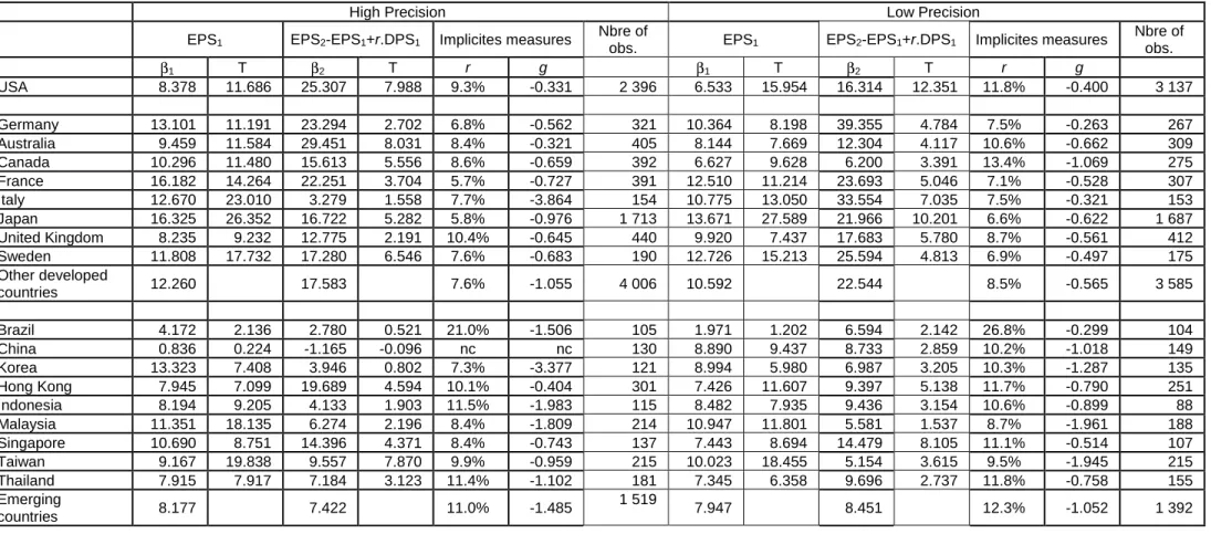
5.2Implied return and precision of forecasts 184
5.3Measure of association and implied rate of return when expected variation of earnings is positive 187
5.4Direct estimates of the rates of persistence of abnormal earnings growth 190
Conclusion 192
General conclusion 201
Summary 206
Annexes 207
Tables and figures 208
General Introduction
This dissertation on emerging markets is driven by the one fundamental question, i.e., is there any association between accounting data and market values in the high-risk and volatile emerging market countries? This topic is important because the investment flows to emerging markets are material1.Net portfolio investment to emerging markets was very small before 1980, the investment started escalating after words. Financial liberalization in 1989 served as lubricant and private portfolio investment exceeded the US$ 10 billion and reaching to US$14.9 billion. Many factors contribute to this rapid development, like; (i) macro economic development and poverty reduction. (ii) cross border capital flows to emerging markets2. According to Dominic Wilson and Roopa Purushothaman of Goldman Sachs3:
• In less than 40 years, the BRICs economies together could be larger than the G6 in US$ terms. By 2025 they could account for over half the size of the G6. They are currently worth less than 15% of the current G6, only the US and Japan may be among the six largest economies in US$ terms in 2050.
• The largest economies in the world (by GDP) may no longer be the richest (by income per capita), making strategic choices for firms more complex.
• As today’s advanced economies become a shrinking part of the world economy, the accompanying shifts in spending could provide significant opportunities for global companies. Being invested in and involved in the
1 Bruner Robert F., Conroy Robert M., Wei Li, O’Halloran Elizabeth F., Lleras Miguel Palacios. (2003).
“Investing in Emerging Markets.” The research foundation of AIMR (CFA Institute). (2003).
2
Global development finance.(2005) p.33-34,p.14.
Capital flows to emerging market economies. (2005). Institute of International Finance. September 24, 2005. Global Financial Stability Report. (2005). International Monetary Fund. September, 2005.
Recent FDI Trends in Emerging Market Economies.(2005) Standard & Poor’s .November 10, 2005.
Battat Joseph and Dilek Akyut.(2005).”Southern multinationals: A growing phenomenon.” IFC, October, (2005).
3 Wilson Dominic, Purushothaman Roopa. (2003). “Dreaming with BRICs: The Path to 2050.” Global
right market – particularly the right emerging markets– may become an increasingly important strategic choice.
In a recent Harvard Business Review article4, Jeffery R. Immelt, Vijay Govindarajan and Chris Trimble have said:
• The model that GE and other industrial manufacturer have followed for decades – developing high-end products at home and adapting them for other markets around the world-won’t suffice as growth slows in rich nations.
• To tap opportunities in emerging markets and pioneer value segments in wealthy countries. Companies must learn reverse innovation: developing products in countries like China and India and then distributing them globally.
• If GE doesn’t master reverse innovation, the emerging giants could destroy the company.
These facts, findings and projections set the stage to understand the investment dynamics in emerging markets. Accounting data plays pivotal role in this regard. In this research, we have studied the link between accounting data and market values mainly Ohlson (Ohlson J., 1995), Feltham and Ohlson (Feltham & Ohlson, 1996), Ohlson & Juettner-Nauroth (Ohlson & Juettner-Nauroth, 2005), and Ohlson & Zhan Gao (Ohlson & Gao, 2006) models keeping in view the specific conditions that prevail in emerging market economies and important to the rest of the world.
According to Ohlson (Ohlson J., 1995) model, the present non-accounting information affects the future abnormal or residual income, autoregressively. The confabulation about the Ohlson model for equity valuation starts from the present value of expected dividend, equating it to price. This is also known as
4 Jeffery R. Immelt, Vijay Govindarajan, Chris Trimble. (2009). “How GE is Disrupting itself.” Harvard
the first assumption of the Ohlson model. Clean surplus relation, that relates book value to net earnings and dividends is cardinal to accounting based valuation models, is the second assumption of the Ohlson (Ohlson J., 1995) model. Linear information model is the third assumption of the model and according to this both abnormal earnings and non-accounting information are autoregressive. To ring the curtain down, the firm’s market value equals its book value adjusted for the current profitability as measured by abnormal earnings and future profitability as measured by other information. In the same token, the Feltham-Ohlson (Feltham & Ohlson, 1996) dissertate how accrual accounting relates to the valuation of firm’s equity and goodwill. Ohlson Juettner-Nauroth OJ (2005) and Ohlson & Zhan Gao (2006) papers’ discuss the relationship of market value to earning and earnings growth.
The interest in this subject is primarily motivated by practical considerations. Investments in the international equity markets have become significant for fund managers worldwide. The use of methods based on comparison of basic observed ratios, for listed companies, between stock prices and expected earnings per share is often considered the most powerful: “EPS forecasts represented substantially better summary measures of value than did OCF forecasts in all five countries examined, and this relative superiority was observed in most industries ” (Liu, Nissim, & Thomas, 2007). Understanding the link between market value and expected earnings is likely to illuminate the investment process in countries where information is more difficult to collect for foreign investors.
The second motivation is theoretical in nature. It focuses on the relationship between book values and market values. The valuation models based on residual earning (R.I.M.) and abnormal earnings growth (A.E.G.) provide a supportive link between expected future earnings, book value of equities and their market
value in the case of RIM, and between expected future earnings, expected dividends and market values in the instance of A.E.G. The pioneer models of Ohlson (Ohlson J., 1995) or of Feltham and Ohlson (Feltham & Ohlson, 1996), for example, suggest a linear relationship between market value, book value of equity per share, expected earnings per share and finally a variable summarizing the effects of other information on the future earnings. The question is whether an extension of the R.I.M models likely to capture the abnormal growth of earnings enabling to establish a link between the book value and market value of equity, at least in certain circumstances.
In case of A.E.G., the pioneering model of Ohlson and Juettner-Nauroth (Ohlson & Juettner-Nauroth, 2005) claims that only the expected earnings for the next two-years and expected dividend are sufficient. The empirical evidence is not conducive to this hypothesis (Gode & Mohanram, 2003), (Penman, 2005). The question is whether an extension of the model A.E.G.(Abnormal Earnings Growth) proposing more fine decomposition of the abnormal earnings growth in volume and intensity provides a better estimate of the link between expected earnings and stock price of a share.
From the perspective of R.I.M., we begin our study by extending the theoretical R.I.M. models. The objective is first to integrate the evolution of abnormal earnings depending upon the type of growth experienced by the firm. The modeling takes into account the possibility of change in the regime of growth at a point in time. It also supposes that the capacity of the firm to conserve the profit for its shareholders, the largest share of wealth created by growth opportunities, depend upon the importance of equity in the balance sheet. Finally, we have been careful not to accept the hypothesis of the relationship called "clean surplus.” By integrating these elements, we hope to improve the
measurement of the relationship between book value of equity and its market value.
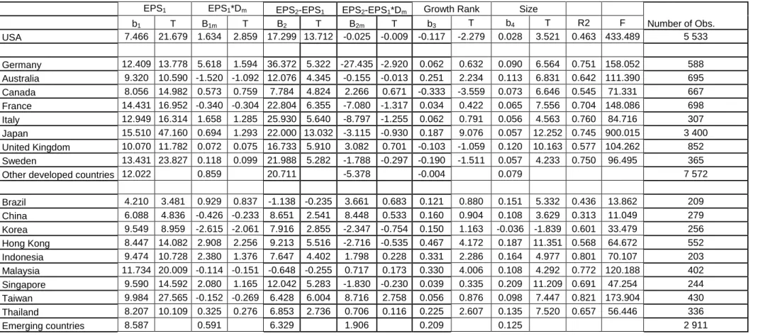
From the empirical stand point, three samples are constructed for the period 1997-2007. They include companies from the United States, other developed countries (Australia, Canada, France, Japan and United Kingdom) and a set of emerging countries (China, Korea, Hong-Kong, India, Malaysia, Singapore, Taiwan and United Kingdom). Our goal is to propose a comparison at international level. From historical accounting data, we construct a synthetic indicator of growth by company. We then proceed to estimate our model by including these variables of growth and other control variables (size, no dividends, year and country). The objective is to verify that the inclusion of the book value of equity not only improves the explanatory power but also the specification of the estimated regression.
From the point of view of A.E.G., we begin our study with a theoretical extension of the model A.E.G. Aware of the fact that the models of type AEG are complex in their inner mechanics (Brief, 2007), we want to make development of the profitability in the form of a progressive realization of a set of growth opportunities. To do this, we take an idea developed by Walker and Wang (2003) in a different context, that of R.I.M. (Residual Income Models). As Walker and Wang, we bring together the microeconomic analysis and modeling of accounting earnings. But we do so as a part of valuation based on taking into account expected earnings and especially their growth.
On the empirical side, three samples are formed over the period 1998-2008. They include American companies, firms from other developed countries (Germany, Australia, Canada, France, Japan, and the United Kingdom) and a set from emerging countries (China, Korea, Hong Kong, India, Malaysia,
Singapore, Taiwan and Thailand). Our objective is to provide an international comparison. From historical accounting data, we build a synthetic indicator of growth by company. We, then, proceed to estimate our model by incorporating the variables of expected earnings (in level and in variation), this synthetic variable of growth and other control variables. The objective is to verify (1) that the anticipated effects of abnormal earnings growth are limited in time, (2) that the inclusion of the synthetic variable for growth makes a significant correction when the variable of growth in the short-term alone is insufficient, (3) that the values implicit of cost of capital are acceptable from an economic stand point.
Emerging market economies is a term coined by Antoine W. Van Agtmael of the International Finance Corporation in 1981of the World Bank, an emerging, or developing market economy is defined as an economy with low-to-middle per capita income. Such countries constitute approximately 80% of the global population, representing about 20% of the world’s economies. Initially, in 1981, the International Finance Corporation’s emerging market index includes only 9 countries; by 20075, the total number of countries had reached to 36. Standard and Poor’s acquired the IFC indexes in January, 2000. The S&P/ IFC index consider a market “emerging”, if it meets the following two criteria:
• It is a low, lower middle, or upper- middle-income economy as defined by the World Bank.
• Its investable market capitalization is low relative to its most recent GDP figures.
The first chapter of this dissertation is theoretical in nature. This chapter presents an introduction to Residual Income valuation (R.I.M.) model and
Abnormal Earnings Growth (A.E.G.) model as put forward by Ohlson (Ohlson J., 1995), Feltham Ohlson (Feltham & Ohlson, 1996), Ohlson & Juettner-Nauroth (Ohlson & Juettner-Nauroth, 2005) and Ohlson Gao (Ohlson & Gao, 2006).This presentation is supported by specific expansion to the model like inflation, default risk and growth opportunities. In the second section of this chapter, we discuss in detail Ohlson (Ohlson J., 1995) and Feltham Ohlson (Feltham & Ohlson, 1996) models with their specific assumptions. This section also contains some particular cases of Ohlson (Ohlson J., 1995) model like growth and firm value, shareholders’ rent and firm value and probability of survival and firm value. In the third section, we discuss inflation, inflation accounting and inflation adjustment of residual income valuation (RIV) as proposed by John O’Hanlon and Ken Peasnell (2004). In the last part of this section, we present through example that the distortion of residual income depends upon the distortion of depreciation which leads us to the conclusion that the more volatile the inflation is, the more uncertain the value of residual income gets, because the accounting system undertaken will be having less time to adapt itself to the abrupt changes of inflation, i.e., the force of Ohlson (Ohlson J., 1995) model diminishes in the volatile inflationary environment. The fourth section of this chapter presents the abnormal earnings growth (A.E.G.) model. The Ohlson Gao (Ohlson & Gao, 2006) paper has been thoroughly discussed.
The second and third chapters are two separate papers. In the second chapter with the title, “The effects of growth on the equity multiples: An international comparison.” We seek answers to two research questions. (i) Is the degree of association between book value and market value of equity a function of growth conditions and mode of financing of the company? (ii) Are these forms of association invariant around the world? The first section of this chapter is an introduction that carries motivation for the research sample selection and
principal findings. The second section presents problematic and model. The source and evolution of Ohlson (Ohlson J., 1995) model to effectuate empirical work has detailed in this section. The third section presents data and descriptive statistics. The number of companies retained are growing from 7149 in 1997 to 17, 376 in 2007. Finally, the observations retained are 10,657 for U.S.A., 21, 290 for other developed countries and 20,604 for emerging countries. Descriptive statistics for the variables; Market value cum Dividend/Total Assets, Book value cum Dividend/Total Assets, Net Income/Total Assets , size and absence of dividend are presented for the three samples, i.e., U.S.A., other developed countries and emerging countries. Section 4 of this chapter extends the estimation of other explanatory variables like synthetic variable of growth inspired by the methodology of Haribar and Yehuda (Hribar & Yehuda, 2008) and the proportion of the phases of growth of the firms in three samples, i.e., U.S.A., other developed countries and emerging countries. The next part of this section introduce to methodologies used to calculate the dirty surplus and breakdown of observations by classes of dirty surplus and geographical zones. The section 5 presents the regression results. At first instance we observe that the irrespective of geographical zone net income is the variable most strongly associated with the market value. And, the introduction of book value of equity increases the explanatory power of the model but also modifies significantly the estimate of earnings and market value of equity. Two results emerge internationally, the low debt and high growth firms are better valued by the investors during the period. When companies are in debt, the growth in earnings does not systematically reflect by the increase in market value of equity. These empirical results confirm the prediction of our theoretical model.
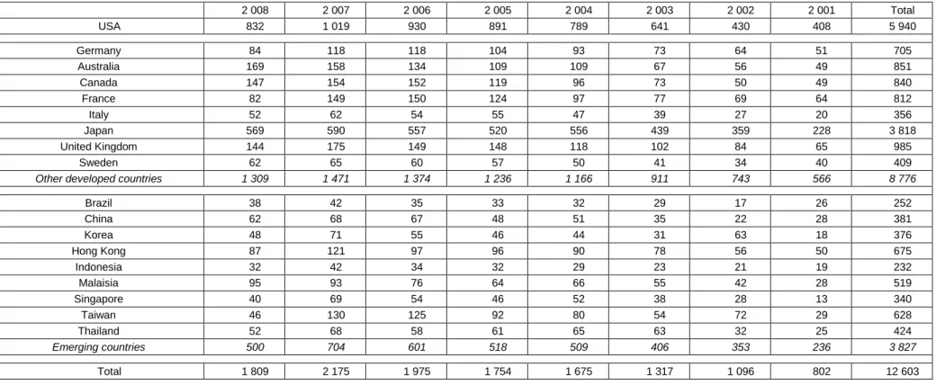
Chapter 3 with the title, “What is the impact of abnormal earnings growth on the market valuation of the companies: An International comparison,” focuses on the following two research questions. (i) Knowing that the form of association
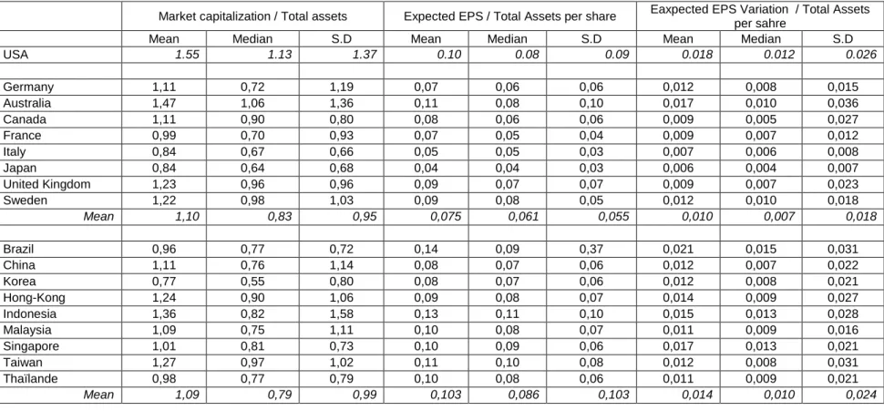
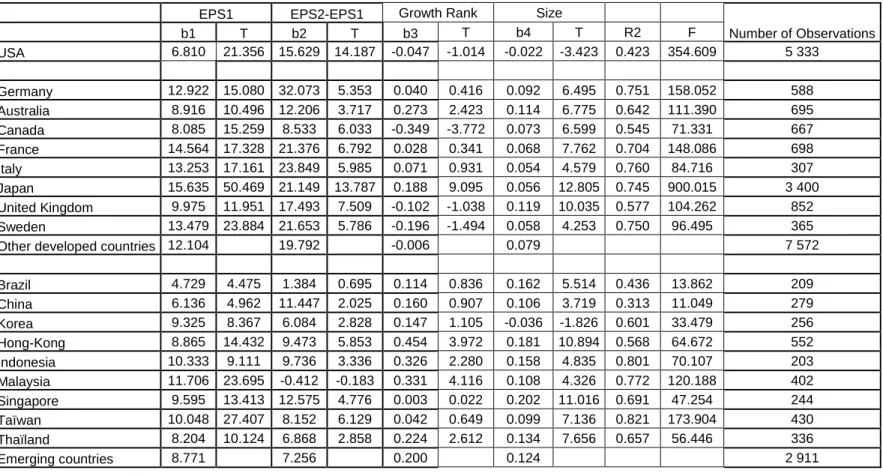
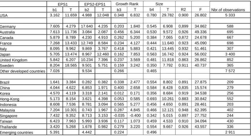
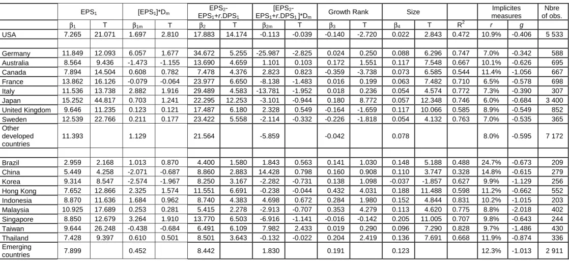
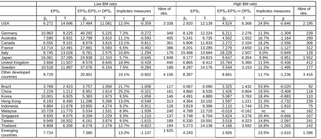
between stock price and expected earnings per share depends on the type of growth of the company, that brings short term increase in expected earnings by financial analysts to explain differences in stock market value. (ii) Can an indicator of growth build on historical accounting data corrects the bias introduced by previous measure? Like chapter 2, the second section of the chapter contains the problematic and model. It introduces the idea developed by Walker and Wang (2003) to A.E.G. (Abnormal Earnings Growth) model to capture growth dynamics of the earnings. The second part of this section holds the development and the third part carries the empirical specification of the model. Data and descriptive statistics have been discussed in the section 3 of the chapter. The data is for the period 1998-2008 and include countries (Germany, Australia, Canada, France, Italy, Japan, United Kingdom, Sweden and USA) and emerging countries (Brazil, China, Korea, Hong Kong, India, Malaysia, Singapore, Taiwan and Thailand). In total, we have 12 603 firm years distributed for 8 776 to other developed countries and 3 827 for emerging countries. The number of observations are increasing over the period : 802 in 2001 and 1809 in 2008. The descriptive statistics are presented in Table 2 of this chapter and discussed in the second part of this section w.r.t., 3 samples and countries. The variable studied include: Market capitalization/Total Assets, Expected EPS/Total Assets per share, Expected EPS variation /Total assets per share, size, variation of sales over 2 years in %, variation of book value of equity in excess of net income over 2 years in % and ratio of investment over 2 years compared to depreciation allowances. Section 4 and Section 5 of this chapter presents the empirical results and robustness tests. The main findings from this research are: irrespective of geographical zone, expected earnings per share remains the variable most strongly associated with the stock market values. But, coefficients are high in developed countries than in emerging countries. At the second instance we note that the PER and PEG ratios combine in valuation, essentially, with in developed countries. These two indicators must be supplemented to
avoid either over valuation or under valuation. Finally, at international level, the expected implied rates of return are significantly higher in emerging countries than in developed countries.
Chapter1: Residual Income (R.I.M.) and Abnormal
Earnings Growth (A.E.G.) Models
Chapter1: Residual Income (R.I.M.) and Abnormal Earnings Growth (A.E.G.) Models
1. Introduction:
This chapter discusses the Residual Income Valuation Model (RIM) and Abnormal Earnings Growth model (AEG) as proposed by Ohlson (1995), Feltham Ohlson (1995), Ohlson & Juettner-Nauroth (2005) and Ohlson and Zhan Gao (2006), respectively. Beside this principal discussion, in this chapter, we propose different expansion to these models with special reference to inflation, default risk and growth opportunities. A long stream of literature on Ohlson (1995) and Ohlson-Feltham (1995) has been sought to understand the theoretical as well as empirical aspects of the models. Before embarking on our journey for the proposed models in this chapter, it is better to understand the Ohlson (1995) and Ohlson-Feltham (1995) models and to know where actually the models stand on evolutionary tree for capital market research.
Fundamental analysis involves study of a firm’s current activities and prospects for the purpose of estimating its value. The objective here is that we know the factors like product demand, corporate strategy, industry outlooks etc. which are not incorporated in the accounting data also affects the firm value. But accounting remains as a base for all firm related decision making and research in accounting data help us to comprehend the fundamental analysis by providing us a link between firm accounts and its value. Hence, the Ohlson (1995) Model.
The technology presented in Ohlson (1995) Model is remarkably simple in nature and very interesting. It is about residual income and non accounting information which are autoregressive. The present non accounting information generates shocks which affect the future abnormal or residual income. Thus, in
plain language, non accounting information generates shocks auto regressively which affects the abnormal earnings auto regressively.
Like Ohlson (1995) Model, the Feltham-Ohlson (1995) Model (FO) concerns how one conceptualizes a firm’s expected growth with the accounting data reflecting its recent performance. As discussed in detail (later) in this chapter, the model presents the market value in terms of financial assets (liabilities), the expected changes in operating earnings, current operating assets and the expected change in operating assets.
While talking of historical background of the Ohlson (1995) and Ohlson-Feltham (1995) models, we find that the work done during 1960’s provided a base for these models. The work of Edward and Bell (1961), Modigliani and Miller (1958), (1961), and Preinreich (1938) is worth to mention in this regard. Later, the contribution by Penman (1997) focuses the capital market research on the relation between accounting data and firm value, i.e., fundamental analysis. Numerous empirical studies based on the models purposed by Ohlson (1995) and Ohlson-Feltham (1995) validate the authenticity of the models. To quote some of them includes the work done by Dechow et al.(1999); Myres (1999) and Morel (2003); etc. Despite the fact that the researchers take some assumption while experimenting the models, the validity and authenticity of the models remains unquestionable.
The third section of this chapter examines Residual Income Valuation (RIV) model in inflationary environment of emerging markets. Various studies, up till now, have demonstrated the accuracy and superiority of RIV on other valuation models. In transitory and growth economies of emerging market countries, inflation is unavoidable. Hyperinflation in some of these countries makes accounting numbers unreliable to infer any sort of investment decision.
Valuation is at the centre-stage and in the spot light for all such decision making. This is the context that forces us to verify the authenticity of RIV in the inflationary and uncertain environment of emerging markets. Discussions about inflation are as perennial as changing climatic conditions. As soon as there is a price hike, intellectuals and professionals resume talking about the issue. Historically, we find that the issue remained in discussion during seventies and eighties quite frequently. Now, the studies on inflation appear once in a blue moon.
Accounting statements provide the input data for all sort of decision making. In the period of inflation, this information has been criticized on the ground that it reflects the number of dollars while the value of the dollar is changing. In short, “Inflation creates an earning illusion by mismatching of expenses based on allocation of historical cost with current revenues in determining earnings. This mismatching distorts mapping of aggregate earnings and book value into equity value such that value relevant information is lost.” Hughs, Liu and Zhang (2004). This comparison of apples with oranges must be avoided. And, to have fair view apples must be compared with apples. Hence, inflation adjustment is necessary.
As for the question of whether residual income valuation (RIV) should be written in terms of inflation adjusted residual income rather than historical cost residual income. Two very recent studies are worth to mention, in this regard. First is the study by Ritter and Warr (RW) (2002) that claims that this practice can lead to miss valuation of firms. RW claim that for residual income models to produce accurate measures of true economic value “they should use real required returns, adjusted depreciation for the distorting effects of inflation, and make adjustment for leverage-induced capital gains” (Ritter and Warr, 2002, pp.59-60). Second, interesting work in this area is by O’Hanlon and Peasnell
(2004). Their work contradicts the work carried out by RW. They argue that in a setting in which accounting numbers and forecasts are normally presented in historical cost terms, the inflation adjustment of RIV is likely to bring unnecessary complications to the valuation process, which increased scope for errors. Their findings are briefly discussed, later, in this chapter.
Emerging market countries are growth economies. This phenomenon of growth makes it impossible to avoid inflation. Countries like Turkey used to have an exceptionally high inflation rate. This difference matters because inflation affects forecasted local cash flows and local discount rates. This is the reason that in certain countries of Latin America for example Brazil, financial statements are published both in nominal and inflation adjusted forms so that the readers can draw the rational inferences.
Comparative to residual income valuation model, which takes historical accounting data as input for equity valuation, earnings, earnings growth is frequently used by analysts for the same purpose. The relationship of market value to earnings and earnings growth is studied through two recent papers, i.e., Ohlson & Juettner-Nauroth (OJ) (2005) and Ohlson and Zhan Gao (2006). The fourth section of this chapter discusses the Ohlson and Gao (2006) paper. This paper is comprehensive in nature in a sense that it discusses the OJ (2005) valuation model and amplifies the results.
The rest of the chapter is arranged as follows. In section two we discuss Ohlson (1995) model and Feltham-Ohlson (1995) model with some particular cases. Section 3 presents the inflation and inflation, inflation adjustment of RIV and empirical inquiries of RIV from nominal, real and pure accounting angles. Section 4 covers the relationship of earnings growth and value and section 5 concludes this chapter.
2.1) The Ohlson Model
In this section we present the relationship between Ohlson Model and classical valuation models, i.e., present value of expected dividend and discounted cash flow and observe that all these models convert to Ohlson (1995) Model.
The discussion about the Ohlson Model for equity valuation starts from the present value calculation of expected dividends.
2.1.1) The Present Value of Expected Dividends.
Under the neo-classical multi-period framework (Fisher 1930), the market value of a firm's equity P (t) at year t equals the present value of expected dividends d (t) discounted at a constant factor R:
[
]
1 ( ) ( ) (PVED) (1) (1 ) E d t P t R τ τ τ ∞ = + = → +∑
Where E [] denotes the expectation operator. This model permits negative d (t) that reflects capital contributions. The d (t) should in fact be referred to as dividends net of capital contribution but we will keep referring it to simply dividends for the sake of brevity. PVED is an equilibrium condition. It is no-intertemporal arbitrage price that results when interest rates are non-stochastic, beliefs are homogeneous and individuals are risk neutral. PVED is also known
as first assumption of Ohlson Model. 2.1.2) Residual Income Valuation:
Central to the accounting based valuation models is the clean surplus relation (CSR) that relates book value bv (t) to net earnings x (t) and dividends.
( ) ( 1) ( ) ( ) (CSR) (2) ( ) ( 1) ( ) ( ) ( ) ( 1 ) ( ) (3) bv t bv t x t d t d t bv t x t bv t d t τ bv t τ x t τ = − + − → ⇔ = − + − ⇔ + = − + + + →
CSR is the second assumption of the Ohlson Model. All the variables on the right hand side of CSR are primitive, so that the current dividend d (t) has no effect on current earnings x (t)
We, now, define residual income ax (t) as the difference between net income and capital charge at the discount rate R:
( ) ( ) ( 1) ( ) ( ) ( 1 ) (RI) (4) ax t x t R bv t ax t τ x t τ R bv t τ = − − ⇔ + = + − − + → → Putting (4) in (3) ( ) ( 1 ) ( ) ( 1 ) ( ) d t τ bv t τ ax t τ R bv t τ bv t τ ⇒ + = − + + + + − + − + ( ) ( 1 ) ( ) ( 1 ) ( ) ( ) (1 ) ( 1 ) ( ) ( ) d t bv t ax t R bv t bv t d t R bv t ax t bv t τ τ τ τ τ τ τ τ τ ⇒ + = − + + + + − + − + ⇔ + = + − + + + − +
Combining (PVED) and (RI) leads us to an alternative representation of the firm’s equity known today as the residual income valuation.
[
]
1 (1 ) ( 1) ( ) ( ) ( ) (1 ) E R bv t bv t ax t P t R τ τ τ τ τ ∞ = + + − − + + + = +∑
[
]
[
]
[
]
1 1 1 ( 1) ( ) ( ) ( ) + 1 (1 ) (1 ) (1 ) E bv t E bv t E ax t P t R R R τ τ τ τ τ τ τ τ τ ∞ ∞ ∞ = = = + − + + ⇔ = − − + + +∑
∑
∑
Residual income is very similar in nature to a project’s NPV and Stewarts’s (1991) EVA (Economic Value Added), i.e., they are a measure of whether the company is creating or destroying value, with the difference that EVA is written
in terms of operating income and book capital while residual income is written in terms of total income and book value.
[
]
[
]
[
]
1 1 1 ( ) ( ) ( ) ( ) ( ) + (1 ) (1 ) (1 ) E bv t E bv t E ax t P t bv t R R R θ τ τ θ τ τ θ τ τ ∞ ∞ ∞ = = = + + + ⇔ = + − + + +∑
∑
∑
[
]
1 ( ) ( ) ( ) (RIV) (5) (1 ) E ax t P t bv t R τ τ τ ∞ = + ⇔ = + → → +∑
This result was originally presented by Preinreich (1938).Equivalently to PVED, RIV shift focus from wealth distribution (dividends) to wealth creation (residual income). Equity valuation reconciles with Modigliani-Miller (1961) theory of dividend irrelevancy through RIV. Residual income valuation also looks attractive to accountants as it reconnects (financial) equity valuation to their long known concept of (accounting) good will, defined as the difference between the market value and book value of a firm.
Directly from the RIV, one can derive the following expression for the firm’s good will g (t):
[
]
1 ( ) g(t) ( ) ( ) (6) (1 ) E ax t P t bv t R τ τ τ ∞ = + ⇔ = − = → +∑
2.1.3) Linear Information Model:
Ohlson contribution lies in the additional specification of the time-series behavior of residual income. A simple linear information model formulates the dynamics of residual income and of information “other than” residual income
( )t
1 2 ( 1) ( ) ( ) ( ) (7) ( 1) ( ) ( ) (8) ax t ax t t t t t t ω ν ε ν γν ε + = + + → + = + →
Where the disturbance terms ε1( )t and ε2( )t are two zero-mean random variable and where the parameters ω and γ are fixed and known in the sense that the firm’s economic environment and accounting principles determine ω and γ .We restrict ω and γ to be positive and less than 1 for stability.
The equation ν(t+1) =γν( )t +ε2( )t also know as the assumption three of the
Ohlson (1995) model. According to this assumption both abnormal earnings and
non accounting information are autoregressive. Further, non accounting information is an additive shock to next period’s abnormal earnings. The non accounting information can be completely unpredictable (γ =0) or partially predictable (γ =1), but it must flow through abnormal earnings in the next period. The distinction between ν( )t and ε1( )t is that the ν( )t is partially forecastable while ε1( )t is completely non-forecastable. Note also that the non accounting shocks to abnormal earnings in period t becomes part of autoregressive process for abnormal earnings (ax (t+1)) going forward. Hence, non accounting information generates shocks auto regressively and these shocks flow through future abnormal earnings autoregressively. In this way the model handles non accounting information very nicely.
More specifically, ν( )t can be re-written as:
[
]
( )t E ax t( 1) ax t( )
ν = + −ω
And thus primarily interpreted as unpredicted growth.
One property of assumption 3 is that paying dividend reduces next periods earning by the amount the rate of interest the firm could have earned on the
assets. To see this, substitute the definition of abnormal earnings into the (ax (t+1) process and rearrange to get the “normal” earning process.
1 ( 1) ( ) ( ) ( ) 1 1
t t
x+ = −R bv t +ωax t +υt +ε +
Recall that paying dividend reduces the current book value but has no effect on current earnings (by the clean surplus relation), so we have:
1 ( ) ( 1) ( ) t E x R d t + ∂ = − − ∂
A dollar of dividends reduces next period’s expected earnings by the interest that could be earned on that dollar. (This last result is also sometimes referred to as Modigliani /Miller or MM property).
Let’s define the 2-by-2 matrix.
(
)
( )
(
)
( )
( )
(
)
( )
1 1 0 1LIM can be expressed as :
ax(t+1) ( )
1 t+1
Under the expectation operator:
ax(t+1) ( ) E 1 t+1 M R ax t R M t ax t R M t ω γ ν ν ν ν = + = + = +
( )
(
)
( )
( )
1 Recursively, we have: ax(t+ ) ( ) E 1 t+ Thus, ( ) ( ) ( ) ax t R M t ax t P t bv t M t τ τ τ τ τ ν τ ν ν ∞ = = + = + ∑
The characteristic roots of the trignol matrix M are and
1+R 1+R
Because the maximum charateristic root is less than one , the above M series converges and:
(
)
( )
(
)
(
)(
)
(
)
(
)(
)
1 1 ( ) ( ) ( ) 1 where 1 1 1 1-M 0 1 1 1Finally the Ohlson Model for equity valuation can be written as: (1 ) ( ) ( ) ( ) ( ) (OM) (9) 1 1 1 ax t P t bv t M M t R R R R R R P t bv t ax t t R R R ν γ ω ω γ ω ν ω ω γ − − = + − + − + = + − + − + − + = + + → → + − + − + −
We conclude that the firm’s market value equals its book value adjusted for current profitability as measured by ax (t) and for future profitability as measured byν( )t .
2.1.4) Discounted cash flows (under risk neutrality) and Ohlson Model:
By definition, ( ) ( ) ( ); ( ) ( ) ( ); ( ) . ( 1); ( ) ( ) ( ) ( 1) ( ) ( 1) ( ) ( ) ( ) (1 ) ( 1) ( ) ( ) bv t oa t fa t x t fx t ax t fx t r fa t c t ox t oa t oa t fa t fa t fx t c t d t R fa t c t d t = + = + = − = − + − = − + + − = + − + −
Where fa t( ) denotes the financial assets net of debt (most probably negative) and oa t( )the operating assets (As from FO Model).
Each asset contributes to earnings:
( ) ( ) ( )
x t = fx t +ax t
Where fx t( ) denotes the financial income and ax (t) the operating income, net of tax. Under risk neutrality, the risk less interest rate r is the rate to be used
throughout the firm. Then, ( ) . ( 1)
fx t =r fa t−
At the end of the period, free cash flow c (t) from operation (net of capital expenditure)
( ) ( ) ( ) ( 1)
c t =ox t −oa t +oa t−
Are transferred to financial assets, leading to the following financial asset relation:
( ) ( 1) ( ) ( ) ( ) (1 ) ( 1) ( ) ( )
fa t = fa t− + fx t +c t −d t = +R fa t− +c t −d t
Finally, PVED and FAR lead to the well-known discounted cash flow formula:
[
]
1 (1 ) ( 1) ( ) ( ) ( ) (1 ) E r fa t fa t c t P t r τ τ τ τ τ ∞ = + + − − + + + = +∑
[
]
[
]
[
]
1 1 1 ( 1) ( ) ( ) ( ) + 1 (1 ) (1 ) (1 ) E fa t E fa t E ax t P t r r r τ τ τ τ τ τ τ τ τ ∞ ∞ ∞ = = = + − + + ⇔ = − − + + +∑
∑
∑
[
]
[
]
[
]
1 1 1 ( ) ( ) ( ) ( ) ( ) + (1 ) (1 ) (1 ) E fa t E bv t E ax t P t fa t r r r θ τ τ θ τ τ θ τ τ ∞ ∞ ∞ = = = + + + ⇔ = + − + + +∑
∑
∑
[
]
1 ( ) ( ) ( ) (DCF) (15) (1 ) E c t P t fa t r τ τ τ ∞ = + ⇔ = + → → +∑
DCF is thus formally equivalent to PVED and RIV under risk neutrality.
2.2) Feltham-Ohlson (1995) Model
The FO paper models how a firm’s market value relates to accounting data that discloses results from both operating and financial activities. Broadly speaking the paper discusses how accrual accounting relates to the valuation of firm’s equity and goodwill. The model takes four “flow” variables: operating earnings, (net) interest revenues(expenses), cash flows, and dividends and three “stock” variables from the balance sheet comprising of (net) operating assets (i.e., marketable securities minus debt), and book value (fa + oa).
Four kinds of analyses are presented in the model. The first set deals with values as it relates to anticipated realization of accounting data. The second set checks
how value depends on contemporaneous realizations of accounting data. The third set verifies asymptotic relations comparing market value to earnings and book values, and how earnings relate to the beginning of period book values. The fourth set examines how conservative accounting influences the response of value to increments in various components of earnings and assets, subject to debits equals credits. Conservatism results in unrecorded goodwill and fundamentally affects the relations examined in the analysis presented in the paper. Goodwill can reflect either the understatement of the value of existing assets or the anticipation of future positive net present value investments.
2.2.1) Relation between value and expectations about future accounting numbers
In this model a firm, in a neo-classical setting, discloses accounting data at date t (t = 0, 1 …), pertaining to its operating and financial activities. The following variables are representative of data:
book value of the firm's equity , date t earnings for period (t-1,t)
dividends , net of capital contributon , date t = financial assets, net of financial obligation, date t
interest reve t t t t t bv x d fa i = = =
= nues , net of interest expenses , for period(t-1, t) operating assets, net of operating liabilities , date t
t
oa =
operating earnings for period (t-1, t)
cash flows realized from operatig activities ,net of investments in those activities , date t
t t ox c = =
Market value of the firm's equity, date t.
t
P =
The model segregates the firm’s activities into financial and operating activities. The book value at date t is bvt = fat +oat and its period (t-1, t) earnings are xt = +it oxt
2.2.1.1) Clean surplus accounting:
The income statement and balance sheet reconciles via the clean surplus relation which is also the first assumption of the FO model and can be given from the
following set of equations:
1 1 1
(CSR) (2) (As presented previously) (FAR) (10) (OAR) (11) t t t t t t t t t t t t t bv bv x d fa fa i d c oa oa ox c − − − = + − → = + − + → = + − →
2.2.1.2) Net interest relation
Net interest relation is the second assumption of the FO model and can be
expressed from the following equation:
1
( 1) (NIR) (12)
t t
i = −R fa− →
It determines the accounting for financial assets so that their book and market value coincide to equal fat for all t.
2.2.1.3) Pt equals PVED:-
[ ]
1 (1) ( presented previously) t t t P R E dτ τ As τ ∞ − + = =∑
→PVED is the third assumption of the FO model, the interpretation is same as of
Ohlson (1995) Model.
Value of equity = Value of Financing Activities + Value of operating Activities = fat +
[
oat +gt]
Goodwill imply towards accounting for operating assets. This is because the financial activities have zero abnormal earning due to NIR.
Unbiased accounting obtains if : E gt
[ ]
t+τ →0 as τ → ∞[ ]
Conservative accounting obtains if: E gt t+τ ⊃0 as τ → ∞
Regardless of the dividend policy and the date t information.
2.2.2) Relation between value and current accounting numbers
This relationship is presented with linear information (fourth assumption of FO
model) dynamics as below:
1 11 12 1 1 1 1 22 2 2 1 1 1 1 2 3 1 2 1 2 2 4 1 (13); (14); (15); (16) a a a t t t t t t t t t t t t t t t ox ω ox ω oa υ ε oa ω oa υ ε υ γ υ ε υ γ υ ε + + + + + + + + = + + + → = + + → = + → = + →
The random terms, εjt+τ satisfy the non-predictability, mean zero, condition
t
E εjt+τ=0, j=1,..., 4 t and τ ⊃0.and a realization of these terms updates the information vector from ( , , 1 , 2 ) to ( 1, 1, 1 1, 2 1)
a a
t t t t t t t t
ox oa υ υ ox+ oa+ υ υ+ + via four above equations.
To make sure the convergence / divergences of these variables, the following restrictions are imposed:
11 12 12
(1)γh p1,h=1, 2; (2)0≤ω p1; (3)1≤ω pR and (4) ω ≥0.
Condition (1) ensures that the random events influencing other information have no long run effect on future other information, i.e., as
[
]
0 , 1, 2.t ht
E υ +τ → as τ → ∞ =h
Condition (2) restricts the (marginal) persistence in abnormal earning. The lower bound ω11 ≥0eliminates implausible persistence. The upper bound ω11 p1, permits positive or zero persistence but that vanishes with time.
Condition (3) restricts growth in operating assets. The lower bound, implies
[
]
[ ]
0 asa
t t t t t t
E oa +τ =E ox+τ = E c+τ = τ → ∞. The upper bound ω22 pR i.e., the requirement is necessary for absolute convergence in the present value calculations of expected abnormal operating earnings and expected cash flows. Condition (4) represents the dichotomous possibilities of unbiased
(
ω12 =0)
versus conservative
(
ω12 f0)
accounting.The valuation function can be expressed as:
(
)(
)
(
) (
)(
) (
)
1 2 11 12 2 1 2 1 2 11 22 11 11 1 2 . (17) where ; , a t t t t t P bv ox oa R R and R R R R R R α α β υ ω ω α α α β β β ω ω ω ω γ γ = + + + → = = = = − − − − − − The valuation function coefficients for operating assets and earnings, α1 andα2 are more important where as coefficient for other information β1 and β2are less significant.
In the same way goodwill can be expressed as:
1 2 . (18)
a
t t t t t
g = +P bv =αox +α oa +β υ →
Unbiased accounting is equivalent to α ω2 = 12 =0;conservative accounting is equivalent toα ω2, 12 f0.
2.2.3) Asymptotic relations among value, value changes, and contemporaneous accounting numbers:
The use of asymptotic relations permits us to abstract from the idiosyncratic effects of information, thereby identifying on average relation. The following three relations are observed in the article:
1) Price/earnings relation; 2) Relation between change in value and accounting earnings;
3) Relation between book value and accounting earnings.
2.2.3.1) Price /earnings relation:
In a world of the conservative accounting, growth firms tend to have larger P/E ratios than no growth firms, and no growth firms tend to have the same ratios as firms using the unbiased accounting.
Conservative accounting
(
ω12 f0)
and growth( )
ω22 imply :(
)
t
E Pt+τ +dt+τ −φxt+τ f0 as τ → ∞
(
)
t
Unbiased accounting or no growth imply
E 0 as : 1 t t t P d x R where R τ τ φ τ τ φ + + + − + → → ∞ ≡ −
2.2.3.2) Relation between change in value and accounting earnings
Conservative accounting
(
ω12 f0)
and growth( )
ω22 imply:(
)
t 1
E Pt+τ +dt+τ −Pt+ −τ −xt+τ f0 as τ → ∞
Unbiased accounting or no growth implies
(
)
t 1
E Pt+τ +dt+τ −Pt+ −τ −xt+τ→0 as τ → ∞
2.2.3.3) Relation between book value and accounting earnings
[ ]
(
)
[
]
(
)
[ ]
(
)
[
]
(
)
[ ]
[
]
t t t t t t t t 11 11 t t ta)E 1 implies ,E 0 and E 0;
)E 1 +K ,K (0, ) implies,E 0 and E 0; 1 )E impliesE 0 and E t t t t t t t t t t t t t t t t t x R bv P bv P d x b x R bv P bv P d x R K R c x P bv P τ τ τ τ τ τ τ τ τ τ τ τ τ τ τ φ φ ω ω + + + + + + + + + + + + + + + → − − → + − → → − ∈ ∞ − + − → − = − → ∞ − f f
(
t+τ +dt+τ)
−φxt+τ f0;Part (a) provides the bench mark relating price in an unbiased fashion to book value and earnings. Part (b) shows a bias in price relative to book value, but not in price relative to earnings. This is because the (expected) goodwill is positive but bounded due to no growth. Part (c) shows biases in both price relative to book value and price relative to earnings, i.e., goodwill grows exponentially, and this leads to understand change in book value.
2.2.4) Comparative dynamics: cash earnings versus accrued earnings
This section examines how an incremental dollar of cash operating earnings versus an incremental dollar of accrued operating earnings affects price. Please consider the following set of equations:
) 1, 1, 0 1. ) 1, 1, 1 0. ) 0, 1, 1 1. t t t t t t t t t t t t t t t t t t a ox c oa x bv fa b ox c oa x bv fa c ox c oa x bv fa ∆ = ∆ = ∆ = ⇒∆ = ∆ = ∆ = ∆ = ∆ = ∆ = ⇒∆ = ∆ = ∆ = ∆ = ∆ = − ∆ = ⇒∆ = ∆ = ∆ = −
The impact of three types of changes on value and future expected earnings depends on whether the accounting is unbiased or conservative. Consider the following statements:
a) the accounting is unbiased;
[ ]
1[ ]
1[ ]
1 ) ; ) 0; ) ; ) 0. t t t t t t t t t t t t t t P P P b caccrued earnings cash earnings investment
E x E x E x
d e
accrued earnings cash earnings investment
+ + + ∂ = ∂ ∂ = ∂ ∂ ∂ ∂ ∂ ∂ = = ∂ ∂ ∂
One replaces the ‘=’ signs in statements (b) through (e) with ‘ f ’ signs if accounting is conservative.
2.2.5) Conservative accounting and zero net present value investments
Goodwill can reflect either the understatement of the value of existing assets or the anticipation of future positive NPV investments. In this case unbiased accounting results in capitalization of the initial investment in operating assets. Conservative accounting, in contrast, results in capitalization of only a fraction of that investment and expensing of the remainder. As a result, conservative accounting, on average, results in low earnings in the early periods and large earnings in the later period.
2.3) Some Particular Cases:
From Ohlson (1995) model presented above we can derive the following set of equations: Noting that 0
[ ]
1 0 0 ~ v X XE a =ω⋅ a + , we can write that
[ ]
a aX X
E
v0 = 0 ~1 −ω⋅ 0. (OM) equation becomes:
(
)
[
]
ω[
ω] [
γ]
[
[ ]
]
[
ω] [
γ]
ω ω − ⋅ − ⋅ ⋅ − + − ⋅ − ⋅ − − ⋅ + − ⋅ − + = R R R BV r X E R R R R D X B r X BV MV0 0 0 0 0 0 0 ~1 0Please note that: 0
MV= Market value of equity
0
BV =Book value of equity.
Rearranging:
[
]
[
] [
]
[
] [
]
[
] [
]
[
] [
]
0 0 0 0 0 1 1 (19) R r R r MV BV X D R R R R R R R E X R R ω γ ω γ ω γ ω γ ω γ ω γ ω γ − ⋅ ⋅ ⋅ ⋅ ⋅ ⋅ = ⋅ − − ⋅ + ⋅ + − ⋅ − − ⋅ − − ⋅ − ⋅ % − ⋅ −The above model present the advantage of attaching market value with two well-known accounting values, i.e., equity and net income, one financial variable total dividend and finally one estimated variable well followed by the analysts, i.e., estimated earnings. It may work for empirical results.
Noting, finally, only the price and some rearrangements the same model can be written as:
[
]
0 1 1[
] [
]
1 0 0 1 (20) E X X X r r r R MV BV R ω r R ω r R ω R γ − ⋅ = ⋅ − + ⋅ + ⋅ − − − ⋅ − % Where X1 =ω⋅[
X0 +(
X0 −D0)
⋅r]
+BV0⋅r⋅(
1−ω)
.We can notice that this model is nothing but an extension of the OM equation.
2.3.1) Growth and firm value for shareholders:
The two preceding models have been developed from the hypothesis about the dynamics of total earnings expressed in monetary units but it is normal to decompose earnings as a product of a volume capital invested and rate of return.
In the previous models, the appraisal is done through capital invested BV. But nothing has been said about evolution of return on equity ROE.
The first model permitting the evolution of ROE. In fact, we can write:
1 and a a t t t t t t t t X X ROE r ROE r B X D B ω + ⋅ = + = + − +
Noting t t t t D X B B c + − = +
1 , the estimated growth in the capital, we get:
[
]
[
ROE r]
c r ROEt ⋅ t − + = − + 1 1 ωIt is clear that nothing is supposed in the previous model on dynamics of c. It may be varying. However, if c varies, it implies a negative variation and perfectly compensates the persistence of increase in ROE and the increase of the growth factor on cost of capital. Is it a reasonable hypothesis? This question can be answered only empirically.
2.3.2) Rent and Firm value for its shareholders:
One of the major critics on the previous modeling is in choosing an autoregressive model for residual income. One supposes that this residual income tends to 0 with time, meanwhile it is difficult to accept this idea that the company can generate investment opportunities at NPV zero. This supposes extremely strong condition of competition.
We purpose the following modeling in terms of ROE.
Posing:
[ ]
[
]
1 0 ~ − ⋅ + = t t t a t k h BV X EWhere kt is the part of ROE in increase of the cost of capital
subject to disappear. And, ht is permanent part.
t h h k k t t t ∀ = ⋅ = + 0 1 δ
Finally supposing constant growth in capital:
( )
c t BVBVt = t−1⋅1+ ∀
And we can write: