July 2011
Institut Supérieur de l’Aéronautique et de l’Espace
Structural Optimization of a
Flexible Wing:
Reduced Model Approach
Final Project
Internship tutors Dr. Joseph Morlier (ISAE/DMSM)
Dr. Miguel Charlotte (ISAE/DMSM)
“Try not to become a man of success
but rather to become a man of value”
4
Abstract
This project contains two parts that the first one is about sizing a wingbox throughout analytical formulas, from a wing of a commercial narrow-body airliner. It is based on structural criteria for a cruise load case taking into account the major forces applied in the wing. It is a useful tool to quickly get first results for an optimization process and a worthy start for a numerical optimization in Nastran/Patran as well, since great results are directly related with right inputs. Beyond the MATLAB codes, a friendly interface from MATLAB has been used, so the user can choose the inputs and then view the results through graphics and table data.
The second part is the construction of a response surface (Surrogate Model) of a wingbox versus a NACA airfoil from sampled NACA parameter. Those surrogate models can be used as a first approach to the final wing thickness results, since they are fast and cheap. The response surfaces are made for the analytical and numerical approaches. Before the surrogates, the Design of Experiments are made with the main objective of analyze the impact of each variable in the outputs. Then, with this study, maybe some variables can be neglected compared with others more critical; consequently, the response surfaces can be created faster than if it was used all inputs.
The entire project is developed with metallic materials; nevertheless, the method for doing the optimization with composites is approximately identical. Remembering that composites are largely used nowadays in aeronautical field.
Keywords: Wingbox, structural optimization, NACA airfoil, Surrogate Model, Design of Experiments
Contents
1 Introduction ... 16
1.1 DMSM ISAE/SUPAERO ... 17
1.2 Internship goals ... 17
2 Wingbox Optimization: Analytical approach ... 18
2.1 Wingbox definition ... 18
2.1.1 NACA airfoils, types, advantages, disadvantages ... 19
2.1.2 Aircraft parameters/ Wing geometry ... 21
2.2 Materials ... 25 2.3 Load Cases ... 26 2.4 Criteria ... 40 2.5 Wingbox Centers ... 44 2.6 Wingbox Sizing ... 46 2.7 Wingbox Analysis ... 51
3 Wingbox Surrogate Model ... 60
3.1 Theory/ Introduction ... 61
3.2 Design of Experiments (DoE) ... 63
3.3 Surrogate Model ... 71
4 Conclusion and Perspectives ... 79
5 References ... 81
6 Appendix ... 83
6.1 Appendix A – MATLAB code of CG and SC ... 83
6.2 Appendix B – Wingbox evolution ... 87
6.3 Appendix C – Function create airfoil in MATLAB ... 91
6.4 Appendix D – Complement Graphics of the wingbox analysis ... 92
6.5 Appendix E – Tables used in the Surrogate Model ... 97
6
Table of Figures
Figure 1 - Non-dimensional wingbox position in airfoil ... 18!
Figure 2 - Wingbox restrictions ... 19!
Figure 3 - NACA parameters represented in NACA 2412 ... 20!
Figure 4 – Schema of WB definition ... 21!
Figure 5 - Wing Geometry parameters [11] ... 23!
Figure 6 - Wing sweep angles ... 23!
Figure 7 - Schema showing the lift coefficient procedure ... 24!
Figure 8 - Framework for the wing geometry definition ... 25!
Figure 9 - Dimensioning load case example [12] ... 27!
Figure 10 – Structural limitation according to the flight envelope [2] ... 28!
Figure 11 - Basic loads [2] ... 29!
Figure 12 - Shear Force, Bending Moment and Torsion positive senses in the Shear Center . 30! Figure 13 – Wing geometry with the references adopted ... 30!
Figure 14 - Fuselage-engine position [4] ... 31!
Figure 15 - Loads creates by the elliptic lift distribution in the wing [4] ... 34!
Figure 16 - Mass distribution in the wingspan [4] ... 36!
Figure 17 - Engine's position in relation with the shear center [4] ... 37!
Figure 18 - Shear Force distribution for a wing with NACA 2420 ... 38!
Figure 19 - Bending moment distribution for a wing with NACA 2420 ... 39!
Figure 20 – Torque distribution for a wing with NACA 2420 ... 40!
Figure 21 - Dimensioning sizing criteria [12] ... 43!
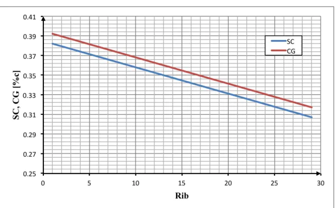
Figure 22 - SC and CG of the Wingbox (Station 16 of a wing with NACA 4420) ... 44!
Figure 23 - Shear Center and Center of Gravity versus Rib ... 45!
Figure 25 - Shear force applied in the wingbox ... 49!
Figure 26 - Wingbox mass, wing span and wing area of the NACA 24XX, with XX=10 to 50 (Case 1) ... 52!
Figure 27 - Wingbox mass, wing span and wing area of the NACA 2X20, with X=1 to 6 (Case 2) ... 53!
Figure 28 - Wingbox mass, wing span and wing area of the NACA X420, with X=1 to 9 (Case 3) ... 54!
Figure 29 - Thickness of each part of the WB in function with the Max Airfoil Thickness and the Station ... 54!
Figure 30 – Wingbox mass of the NACA 2XYY, with X=1 to 6 and YY=10 to 50 (Case 4) . 55! Figure 31 - Wingbox mass of the NACA XY20, with X=1 to 9 and Y=1 to 6 (Case 5a) ... 56!
Figure 32 - Wingbox mass of the NACA XY20, with X=1 to 5 and Y=1 to 6 (Case 5b) ... 56!
Figure 33 - Wingbox mass of the NACA X4YY, with X=1 to 9 and YY=10 to 50 (Case 6a) 57! Figure 34 - Wingbox mass of the NACA X4YY, with X=1 to 4 and YY=10 to 50 (Case 6b) 57! Figure 35 - WB Thickness along the wing for the NACA 2415 ... 59!
Figure 36 - WB Thickness along the wing for the NACA 2620 ... 59!
Figure 37 - WB Thickness along the wing for the NACA 3415 ... 60!
Figure 38 - Surrogate Model purpose ... 61!
Figure 39 - Surrogate-based optimization framework [8] ... 62!
Figure 40 - Design of Experiments GUI ... 65!
Figure 41 - Main Variables’ influence in the Upper Skin ... 66!
Figure 42 - Main Variables’ influence in the Lower Skin ... 66!
Figure 43 - Main Variables’ influence in the Front Spar ... 67!
Figure 44 - Main Variables' influence in the Rear Spar ... 67!
Figure 45- Variable's influence in the Upper Skin ... 68!
Figure 46 - Variable's influence in the Lower Skin ... 69!
Figure 47 - Variable's influence in the Front Spar ... 69!
Figure 48 - Variable's influence in the Rear Spar ... 70!
8
Figure 50 – Slices of the Response Surface of each part of the wingbox ... 72!
Figure 51 - Relative Error distribution for the Upper Skin Surrogate Model ... 74!
Figure 52 - Relative Error distribution for the Front Spar Surrogate Model ... 74!
Figure 53 - Relative Error distribution for the Rear Spar Surrogate Model ... 75!
Figure 54 - Relative Error for the Upper Skin with 2 surrogate models ... 76!
Figure 55 - Relative error of the Upper Skin Surrogate Model of the Numerical Results ... 78!
Figure 56 - Relative error of the Lower Skin Surrogate Model of the Numerical Results ... 78!
Figure 59 - GUI of WB Version 1.0 ... 87!
Figure 60 - GUI of WB Version 2.0 ... 88!
Figure 61 - GUI of WB Version 3.0 ... 89!
Figure 62 - Sub GUI of WB Version 3.0 ... 89!
Figure 63 - WB Thickness along the wing for the NACA 2420 ... 92!
Figure 64 - WB Thickness along the wing for the NACA 2520 ... 92!
Figure 66 - WB Thickness along the wing for the NACA 4415 ... 93!
Figure 67 - WB Thickness along the wing for the NACA 4420 ... 94!
Figure 68 - WB Thickness along the wing for the NACA 4430 ... 94!
Figure 69 - Upper Skin Thickness along wing for 9 airfoils ... 95!
Figure 70 - Lower Skin Thickness along wing for 9 airfoils ... 95!
Figure 71 - Front Spar Thickness along wing for 9 airfoils ... 96!
Figure 72 – Rear Spar Thickness along wing for 9 airfoils ... 96!
Figure 71 - Relative error of the Front Spar Surrogate Model of the Numerical Results ... 99!
Tables
Table 1 - NACA 4 digit-series characteristics ... 20!
Table 2 - Weight breakdown ... 21!
Table 3 - Non-dimensional wing ... 21!
Table 4 - Material's properties ... 25!
Table 5 - Load Cases ... 26!
Table 6 - Load Case adopted ... 27!
Table 7 - Airworthiness Requirements for determining the maximum load factor ... 28!
Table 8 - Historical motors position ... 31!
Table 9 - Criteria for each part of the WB ... 41!
Table 10 - Input variables levels ... 64!
Table 12 - Main Variables' influence ... 68!
Table 13 - Reduced Model Coefficients for each part of the WB ... 73!
Table 14 - Root Mean Square Error of each part of the WB ... 73!
Table 15 - Root Mean Square Error of the surrogate ... 77!
Table 15 - Taguchi's Table ... 97!
10
Abbreviations
CERFACS Centre Européen de Recherche et de Formation Avancée en Calcul Scientifique
CNES Centre National d'Études Spatiales
DMSM Département Mécanique des Structures et Matériaux
DoE Design of Experiments
EADS European Aeronautic Defence and Space Company
FAR Federal Acquisition Regulation
GUI Graphical User Interface
IMT Institut de Mathématiques de Toulouse
ISAE Institut Supérieur de l’Aérinautique et de l’Espace ITA Instituto Tecnológico de Aeronáutica
LE Leading Edge
NACA National Advisory Committee for Aeronautics
ONERA Office National d'Études et de Recherches Aéronautiques
OSYCAF Optimisation d'un système couplé fluide-structure représentant une aile flexible
SNECMA Société Nationale d'Étude et de Construction de Moteurs d'Aviation
RMSE Root Mean Square Error
STAE Sciences et Technologies pour l’Aéronaqutique et l’Espace
TE Trailing Edge
Nomenclature
AC Aerodynamic center AR Aspect ratio b Wing span BM Bending moment CG Center of gravity CL Lift coefficientAirfoil slope lift coefficient Wing slope lift coefficient Cmprofil Airfoil moment coefficient
Cr Root chord
Ct Tip chord
D Drag
df Vertical distance between engine center of thrust and shear center
dm Horizontal distance between engine center of mass and shear center
E Young elastic modulus
F Engine thrust
g Gravity
H Altitude
12
J Current rib in study
Kc Buckling coefficient due to compression
Ks Buckling coefficient due to shear
L Lift
Lcg-sc Shear center-center of gravity distance LSL-AC Shear center-aerodynamic center distance
m Maximum camber in percentage of the chord
Ma Bending moment due to aerodynamic efforts
Mengine Engine mass
Mfuel Fuel mass
Mm Bending moment due to inertial efforts
MN Normal mach
MTOW Maximum takeoff weight
Mwing Wing mass
Cruise mach
n , nz Critical load factor
NR Number of ribs
nz cl Extreme load factor
p Position of maximum camber in percentage of the chord Front Spar Shear Flow
Rear Spar Shear Flow
QT Shear flow due to torsion force
r Skin-stringer area retro
S Wing area
Sa Shear force due to aerodynamic efforts
SC Shear center
SF Security factor
SF Shear force
Sm Shear force due to inertial efforts
T Torque
t Maximum Thickness in percentage of the chord
Front Spar Thickness Rear Spar Thickness
Ta Torque due to aerodynamic efforts
te Effective stringer-skin thickness
tSK Skin thickness
Va ,V Speed
W Weight
XL Lower skin horizontal coordinate of the airfoil XU Upper skin horizontal coordinate of the airfoil
y Coordinate along spanwise
Y Normalized coordinate along spanwise
Yc Vertical Coordinate of the camber line (mean line) YL Lower skin vertical coordinate of the airfoil
14
YM Engine position along spanwise
Yt Relative Position of the airfoil skin related to the mean line YU Upper skin vertical coordinate of the airfoil
Geometric angle of attack
0 Zero angle F Fuselage angle Dihedral angle Wingbox area A Angle fuselage-wing SK Skin area ST Stringer area Taper ratio
c Plasticity reduction factor
s Plasticity reduction factor
θ Local angle of the camber line
Taper ratio
Wing sweep angle at 25% of the chord
LE Wing sweep angle in the leading edge
Poisson ratio
Density
Tension stress
comp Compression stress
( comp)cr Critical compression stress
m Torque due to inertial efforts
max Maximum stress applied under tension and shear
y Yield strength of material
Twist angle
xy Shear stress
16
1
Introduction
In order to achieve a structural optimization of a flexible wing, it is developed here two important tools for that: an analytical approach and the development of a reduced model. It is worth to know that this project is just a piece of OSYCAF, which is a huge scientific project, co-funded by the STAE foundation. OSYCAF is a 36 months project started in 2010 supported by some partners based in Toulouse such as CERFACS, IMT, ISAE and ONERA.
Following the aim of structurally optimize a wingbox of a narrow-body commercial airliner, the first part of this study is to get the first good results by analytical formulas. In that way, it will give a wingbox sizing for any airfoil chosen. Before going directly in the point, it is indispensable to have a good background study and to take decisions that define what this optimization are dealing with. For that, the initial chapters contain researches, ideas and judgments that validate the analytical approach made afterwards.
More specifically, this project starts with the definition of which wingbox is going to be studied and the evaluation of the airfoil type to be used, until this time everything is non-dimensional. Then, the airplane details and wing geometry used are exposed and well discussed. After that, it is presented the study of materials, load cases and criteria, defining the conditions and restrictions applied in the wing leading the study to almost a real case.
Later, it is estimated the position of shear center and center of gravity, that impacts on the loading application in the wing. Finally, the results are reached in wingbox sizing, showing an overview of the wingbox evolution study in appendix and a coherent analysis of these results for further discussions. It is relevant to stress that these analytical results are extremely vital for the numerical optimization process using Sol200, whereas this algorithm has high sensibility answers according to the inputs, for this reason, they should be the most accurate as possible.
Throughout the second part, the idea is to build up a surrogate model (response surface) that provides a faster wingbox result if it is given the inputs parameters: the airfoil variables and the wing station. Although, previously, a good strategy is to analysis the variables impact in the outputs, viewing a worthy opportunity to eliminate an input parameter and predicting some conclusions. All that is helpful to achieve a global understanding and most of times save time and reduce costs.
After the Design of Experiments (DoE), usual designation for this first phase of a response surface construction, the surrogate model is constructed. The goal of that is to get fast wingbox results, avoiding time processing in a numerical and analytical approach, therefore the optimization process will be better progressed.
1.1 DMSM ISAE/SUPAERO
The department has the aim of providing skills for ISAE in solid mechanics, so it has an important educational purpose. Although the laboratory is also well known by its researches. They are basically separated in four areas: Damage to composite materials in aerospace structures; Fatigue of metal materials and structures; Dynamics of Structures; Advanced numerical methods for mechanics.
Allying competence and ability, DMSM is a reference on its area being granted by many partnerships. The researches have contracts and collaboration of industries such as Airbus, Astrium, CNES, EADS, Eurocopter, ONERA, SNECMA, Thales Alenia Space.
1.2 Internship goals
The objectives of this project is logically related with the reasons of the OSYCAF project, but more than that, it is strongly connected with the numerical optimization made by other member of this subject in DMSM office, Francisco Habib, who shared and discussed many points, keeping a natural development and coherence to the two internship programs.
As announced before, the goals consist mainly in two. The first of them is to provide realistic analytical results for the wingbox of a flexible wing, which are used for the input numerical optimization. Throughout that tool, it is possible to build a wingbox from any airfoil, remembering that here the focus is on NACA airfoils, nevertheless it is quite easy to modify for any other airfoil.
18 The second goal is the construction of the response surface (surrogate model) that relates the NACA parameters input and variables with the wingbox thickness. It is a useful instrument that can save a lot of time in an optimization process and it is widely used in the industry since its feasibility and simplicity.
2 Wingbox Optimization: Analytical approach
2.1 Wingbox definition
In the process of wingbox (WB) construction, it is imperative the definition of parametric functions and the freezing of some properties and variables. For that, it has been chosen NACA airfoils and a simplified wingbox that is compound by 2 spars and 2 skins (reinforced by stringers). With the aim of parameterize the wingbox, the front spar is defined as 20% of the airfoil chord distance from the leading edge (LE), and the rear spar is at 40% of the airfoil chord distance from the trailing edge (TE). Then, the upper and lower skins are just bars connecting upper and lower corners, respectively. The following figures 1 and 2 better illustrates the non-dimensional wingbox constructed.
Figure 2 - Wingbox restrictions
2.1.1 NACA airfoils, types, advantages, disadvantages
For this study, it was essential to well delineate the airfoils to be studied. The idea of NACA airfoils is pleasant since they are well known and easy to be constructed. Another reason for that choice is the simple integration of the analytical model with the numerical model, because it can better deal with closed equations of NACA variables. All it should be done is set the parameters that create them. For the case of NACA four-digit series is simply defined by the maximum camber (m), position of maximum camber (p) and maximum airfoil thickness (t), so then, the airfoil surface is found by using these three parameters in the following analytical equations.
20
Figure 3 - NACA parameters represented in NACA 2412
The first digit of the NACA four-digit series represents the maximum camber (m) in percentage of the chord (airfoil length); the second specifies the position of the maximum camber (p) in percentage of the chord divided by ten; the last two numbers indicates the maximum airfoil thickness (t) of the airfoil in percentage of chord. By this definition is quite easy to identify the name of those NACA airfoils:
NACA XYZZ, where X = m, Y = p/10 and ZZ = t
This family of NACA airfoils has some advantages, disadvantages and applications associated, all that information is presented in the table 1.
Table 1 - NACA 4 digit-series characteristics
Advantages Disadvantages Applications
Good stall characteristics Low maximum lift coefficient General aviation
Small center of pressure movement across
large speed range Relatively high drag Horizontal Tails
Roughness has little effect High pitching moment Supersonic jets
Figure 4 – Schema of WB definition
2.1.2 Aircraft parameters/ Wing geometry
A general study should also focus in a few variables, letting the other parameters fixed. In this case, it is chosen an airplane, classified into the general aviation, so it is known the weight breakdown, speed, engines power and others elements which will be exposed in the appropriate part of this project. Although it is important to note that the wing is not fixed, since it is variable according to the airfoil chosen. In that way, the Matlab code has the freedom of quickly change the airfoil, and consequently, the wing as well.
It is considered that the airfoil is the same all over the wing. Another restriction is that the number of ribs is fixed as 29, which means 28 wing sections equally spaced.
Table 2 - Weight breakdown
MTOW [kg] Wing [kg] Fuel [kg] Engine [kg] Empty weight [kg]
54229 4510 0 to 13643 2710 40586
Before explaining the reason that a wing is modified every time that an airfoil is changed, it is essential to design the non-dimensional wing by using the following parameters:
i. Taper ratio ( ) ii. Aspect ratio (AR) iii. Dihedral angle ( ) iv. Twist angle
v. Wing sweep at 25% of the chord ( )
Table 3 - Non-dimensional wing
Taper Ratio Aspect Ratio Dihedral Angle [°] Twist Angle [°] Wing sweep at 25%c [°]
22
After that, if the wing area is known, all wing dimensions are defined by the equations below and by the geometric relations, which are exposed in the following figures, giving a complete wing sizing.
Figure 5 - Wing Geometry parameters [11]
Figure 6 - Wing sweep angles
However, the major problem at this time is the wing area, since it has dependence with the airfoil choice. By the assumption of lift equals weight in cruise level, it should find the wing area and lift coefficient that provides the necessary lift. Therefore the way to solve that is: first, choose an airfoil which can be assumed as thin airfoil and so the airfoil slope lift coefficient is 2π; second, calculate the wing slope lift coefficient by the equation 14. After that, knowing the geometric angle of attack and the zero angle, it is possible to calculate the
24 wing lift coefficient, equation 17. The geometric angle of attack is the sum of the fuselage angle (angle between fuselage axis and horizontal axis) and the angle between the wing neutral axis and the fuselage . Both of them is adopted as 1°, usual values for the narrow-body commercial airliner, so then, the geometric angle used is 2°.
Finally, the wing area is given by the equation 18 – the following diagram shows all that method. Reminding that the zero angle is calculated by equation 15, just with the NACA coordinates points.
Figure 8 - Framework for the wing geometry definition
2.2 Materials
It is really important to be aware of what materials are used. Proceeding a search of the previous aircrafts and what is the current tendency, the traditional materials for this class of airplane is metallic, although the latest airplanes are using composites more and more. So then, two materials have been chosen for the wing box:
i. Al 7150 T7751 – Upper Skin and Upper Stringers
ii. Al 2024 T351 Bare – Lower Skin, Lower Stringers, Front Spar, Rear Spar and Ribs Their properties are expressed in the table below:
Table 4 - Material's properties
E [MPa] σy [MPa] ρM [kg/m3]
Al 7150 T7751 71016 - 2823
Al 2024 T351 Bare 73774 290 2768
26
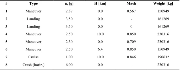
2.3 Load Cases
Naturally, a detailed design phase normally use a huge number of load cases, nevertheless just a few cases of them are actually important for a preliminary design. Moreover, between the eight static cases in the table below, only one of them is used in this study. The purpose of that is to achieve a faster result and also less complex computations. In contrast, this simplification does not invalidate the study, because the option of cruise load case is among the most relevant load cases, which can be seen in the figure 9, in other words, it is a trade-off between precision and time. Besides that, it will also be imposed a minimum thickness limit for all parts of the wingbox, 1mm [6]. As a result, the wingbox sizing will be a great first overview of the wingbox thickness in this project’s phase.
Table 5 - Load Cases
# Type nz [g] H [km] Mach Weight [kg]
1 Maneuver 2.87 0.0 0.567 150949 2 Landing 3.50 0.0 - 161269 3 Landing 3.50 0.0 0 161269 4 Maneuver 2.50 10.0 0.850 230316 5 Maneuver 2.50 0.0 0.709 230316 6 Maneuver 2.50 6.4 0.850 150949 7 Cruise 1.00 10.0 0.846 190632 8 Crash (horiz.) 6.00 0.0 - 230316 Ref. [5]
Figure 9 - Dimensioning load case example [12]
According to the table above, the load case considered here would be the fourth case: Maneuver, load factor of 2.5, cruise altitude, cruise Mach and MTOW, but it was verified that if we consider empty fuel, the loads applied in the wings are more critical then earlier, since the fuel relieves the efforts of bending moment. Thus, it is consider the MTOW to evaluate the necessary lift, even if the wing fuel is zero. After these considerations, the load case implemented is in the next table but it should still specify many aspects before showing the final equations employed.
Table 6 - Load Case adopted
# Type nz [g] H [km] Mach Weight [kg]
1 Maneuver 2.5 12.5 0.79 54229
It is worthy to see the distribution load factor (figure 10) to get an idea of what efforts the airplane is exposed in maneuvering. As showed in the graphic, between the limit load factor and the ultimate load factor, it is the structural damage area and after the ultimate load factor, it is the structural failure.
28
Figure 10 – Structural limitation according to the flight envelope [2]
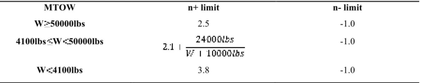
So then, observing the n-V diagram, the aircraft in the cruise speed is limited by structural limit. Therefore, by the table below, the positive critical load factor (nz) of 2.5 is coherent for a cruise phase. As the standard regulation in aeronautical structures, it is assumed a security factor of 1.5, with this in mind; the extreme load factor (nz ce) is 3.75, following the FAR 25.303 regulation and equation 19.
SF
Table 7 - Airworthiness Requirements for determining the maximum load factor
MTOW n+ limit n- limit
W 50000lbs 2.5 -1.0
4100lbs W 50000lbs -1.0
W 4100lbs 3.8 -1.0
The aircraft suffers the influence of several loads arising different origins and reasons, and the heart of the aircraft, wings, suffers as well. Pondering the field of study, it is wise to concentrate in some of them. To give an example, it has the drag, an aerodynamic force, but as it is known the L/D ratio of a commercial airliner is between 15 and 20, so it is evident a significant difference between the drag and lift force. As a consequence, it is reasonable the assumption of not consider the drag in this work. Moreover, the torsional moment due to drag is negligible comparing with the one caused by the lift, because the lever arm of the lift is bigger than the lever arm of the drag.
By computing the aerodynamic, fuel, engine forces and structure weight then it is possible to acquire the wingspan distribution of the basic loads with defined referential points. The basic loads are:
i. Shear ii. Torsion iii. Bending
iv. Axial (Tension and Compression)
The aircraft structures are exposed by different loads, that can be just the influence of basic loads or the association of them, the last case is the most common and for that, it should have a special attention of how to manage the structures sizing computing these loads at once.
30 In the wing, these loads are spread-out, especially in the wingbox, where the intensity and importance of them is vital for the airplane workout, since it holds the most part of loads applied in the wing. Along the wingspan, it has the distribution of shear force, bending moment and torsional moment, parameters that later will define the wingbox thickness. As mentioned before, it should measure the aerodynamic loads, inertia loads such as fuel, landing gear and engine to obtain these distributions.
Figure 12 - Shear Force, Bending Moment and Torsion positive senses in the Shear Center
The wing is studied with a reference in the leading edge of the wing root. As the wing behavior is symmetric, then the results are just for one wing, and so, it is used the semi-span. As a consequence, the equations are based on the y coordinate that is the non-dimensional distance from the origin adopted as the following equation and figure explain.
Figure 13 – Wing geometry with the references adopted
S
FT
BM
SC
y
x
b/2
C
rC
tAnother important non-dimensional parameter is the fuselage-engine distance, which is generally around one third of the semi-span as follows.
Figure 14 - Fuselage-engine position [4]
Table 8 - Historical motors position
Airplane Ym B737-200 0.35 B757-200 0.34 B767-200 0.34 B777-200 0.33 DC10 0.34 MD11 0.31 A300 0.35 A310 0.35 A318 0.34 A319 0.34 A320 0.34 A321 0.34 A330 0.30 Bi-motors average 0.34 Ref. [4]
Finally, all loads will be placed in the shear center of the section, which means that it should know the centers positions of: center of gravity, aerodynamic center and shear center. For that, a MATLAB code is developed, but it has dependence with the wingbox results, as a result, at a first moment these parameters will be estimated based on historical airplanes data.
32 AERODYNAMIC LOADS
The wing that generates an elliptic lift distribution has the minimum induced drag. In order to precisely make it, the wing should have an elliptic geometry, but it is also possible to achieve this lift distribution by the construction of a trapezoidal wing, which has adequate values of taper ratio, twist angle and wing sweep. In other words, for the trapezoidal wing, it ought to find a chord law and an airfoil lift coefficient that give an elliptic behavior.
For the aerodynamic loads, just the lift is taken in account, so the shear force due to aerodynamic efforts is simply the integration of the lift distribution.
The integration in equation 24 is possible through Maple and so then, the aerodynamic shear force can be analytical expressed.
Adding the equation 20, the equation above becomes like:
For the aerodynamic bending moment, the elliptic lift distribution creates a bending moment in all points y as follows.
34
Figure 15 - Loads creates by the elliptic lift distribution in the wing [4]
For the torque due to aerodynamic efforts computation, it needs the knowledge of the centers positions (shear center and aerodynamic center) of each section. Although, only after the construction of the wingbox, the centers can be found, so the way-out of this issue is to suppose 25% of the chord for the aerodynamic center (AC) and an initial approach of 39% of the chord for the shear center (SC), then, this value will be replaced by the equation developed in the Wingbox Centers (section 2.5).
The mathematical approach here is much more complicated, then, as well done in the reference [4], just the final equation is presented. It is compound of two terms: one due to the
airfoil coefficient moment and the other one is due to the lift force position (in the AC) compared with the SC, because all the loads are analyzed in the shear center.
INERTIAL AND ENGINE LOADS
The goal is to optimize the wing mass through a better wingbox, but in this section is clearly evident that for the application of inertial loads, it should specify the wing mass, even if all sizing is not ready for precisely know that. Consequently, it is estimated as the preliminary design in the airplane project, an approach totally confident and highly accurate.
For the distribution of wing mass and fuel mass, it should choose a valid expression and, if possible, easy to implement. The idea is to get the same distribution used for the lift, since more a wing resists heavier efforts, more it will support the inertial loads. By the way, this method is used for the airplanes HALE in the reference [9].
So, for the mass shear load and the mass bending moment the analytical expression is as follows. Recalling that the engine position is placed at one third of the semi-span, for this reason, the distributions are different before and after this point.
36
Figure 16 - Mass distribution in the wingspan [4]
About the torsion due to the mass distribution, it must know the distances between the center of gravity and shear center, the point reference for this approach. Those centers are initially approximated as 38% and 39%, respectively, and as mentioned before these values will be improved by the equations in Wingbox Centers (section 2.5). But in fact, the center of gravity calculated from the wingbox has a systematic error of 4% of the local chord in relation of the center of gravity of the section [4], so the actual equation is presented below. Moreover, the engine generates torsion, since its placement clarified in the figure below, which is not at the same line of the shear center.
Figure 17 - Engine's position in relation with the shear center [4]
Remembering that the engine thrust is 14358 N for each and the values of its position
are: and .
FINAL EQUATIONS
In order to simplify the previous equations and better understand the case as a global view, the following equations summarize all the study made in this chapter. Before that, the lift is considered, as explained before the amount of MTOW times the extreme load factor as follows.
Shear Force
38
Figure 18 - Shear Force distribution for a wing with NACA 2420
Bending Moment
Figure 19 - Bending moment distribution for a wing with NACA 2420
Torque
40
Figure 20 – Torque distribution for a wing with NACA 2420
The study of the wingbox, based on the assumptions and conclusions of the previous chapters, clearly indicates the stress experienced by each part of the wingbox. All of them have the shear stress, and then, the upper skin and lower skin have compression and tension stress, respectively. Founded on that and the reference [5], the succeeding criteria have been chosen for an analytical approach.
Table 9 - Criteria for each part of the WB
Stress Criteria Formula
Upper Skin Compression Stress + Shear Stress
Material yield or local buckling Lower Skin Tension Stress + Shear
Stress
Maximum distortion energy yield Front Spar Shear Stress Shear criterion
Rear Spar Shear Stress Shear criterion
For a more detailed explanation, the following paragraphs explain the formulas adopted.
Upper Skin
The buckling criteria for a combination of stresses is measured as presented in [2].
The critical buckling stress in compression, , is the lowest value among the allowable yield stress of material, the local skin buckling compression and the crippling stress. For the critical buckling stress in shear, , it is the inferior value between the allowable shear stress of material and the local skin buckling shear.
42 The criteria chosen for the lower skin is to meet the requirement of maximum distortion energy yield (failure) under tension and shear stress.
is the yield strength of material and the is the maximum stress applied under the combination of tension and shear stress.
Front Spar and Rear Spar
The criteria adopted for the rear and front spar is the identical, using the shear criterion.
Where the critical stress in shear, which is the smallest value of the allowable shear stress of material and the local buckling shear.
Just for validate the criteria used in this study the following figure shows the dimensioning criterion of the wing from the reference [12]. It indicates that the buckling criteria and the minimum technological thickness of the material define the majority of the thickness wingbox sizing. Therefore, the criteria adopted are coherent for further analyses.
44
2.5 Wingbox Centers
The application of forces in the wing requires the knowledge of its position, for well evaluate the torsional moments. For that information, as mentioned in the Load Cases chapter, for each section, it has three important points:
i. Aerodynamic center (AC) ii. Center of gravity (CG) iii. Shear center (SC)
Figure 22 - SC and CG of the Wingbox (Station 16 of a wing with NACA 4420)
In the AC, the lift force is applied. Then, in the CG, it has the wing and fuel loads. In a first moment, these parameters AC, CG and SC are not correctly known for the computation of the load cases. So, the alternative is to give a first approach for them, calculate the wingbox and then, find the real placement of each factor with a MATLAB code presented in appendix A.
One significant detail to mention is the assumption of just considering the horizontal position of the wingbox centers for the wingbox sizing afterwards. Even if the vertical position of these points are not at the airfoil neutral line, it not changes the forces and moments, except for the amount of moment generated by the engine thrust, nevertheless, it is considered that the difference would be not so relevant among actual moments calculated.
By the first results of the wingbox, the CG and SC were found for each section, and a parameterized equation was made with the intention of replace the initial shots. It was analyzed different airfoils and the sensibility of these parameters with the change of airfoils. After that, a reasonable methodology was found to be a linear fit regression that passes nearby
for all the cases studied, and will allow a faster MATLAB code without recurring to a iterative method which would take longer and results approximately quite the same. Therefore, the equations used are exposed below and a graphic represents it as well.
46
2.6 Wingbox Sizing
After defining the criteria and load case to be used, the analytical approach is ready for use. The goal is to find the thickness for each part of the wingbox. So the idea is to apply the criteria and find an expression for the thickness and what is done below is that.
An essential aspect here is that, although the considered wingbox to optimize is compound of skins and spars, the stringers cannot be neglected. As a result, it is taken from the literature the usual stringer-skin area ratio of 1. In other words, in a section, the upper skin area is equal to the sum of area of all stringers at that section. The stringers have an essential role of taking a great part of the bending moment efforts, minimizing the efforts that go to the skins, so the skins are relieved.
Upper Skin
With the equation 52 from the Criteria chapter, it should take the limit case, so:
Figure 24 - Upper Skin dimensions for sizing
y1 y2 θ t d a Reference Axis
By the utilization of the equations below, the final equation to find the upper skin thickness can be achieved with the material defined in section 2.2.
Compression stress at the upper skin:
Second moment of inertia:
Combining the previous equations:
The critical local buckling stress is defined as follows, using , = 4 and .
For the shear stress, the equation is:
And for the critical shear buckling stress, with , = 5.4 and .
48
Lower Skin
As made for the upper skin, the lower skin has to take the limit case of the criteria and then find the thickness equation as follows.
The yield strength of material is 290 MPa as mentioned in the section 2.2. Then, with the maximum tension stress:
After that, like for the upper skin, the tension and shear stress are found from the equations 61,66 and 67. So, as before:
Front Spar and Rear Spar
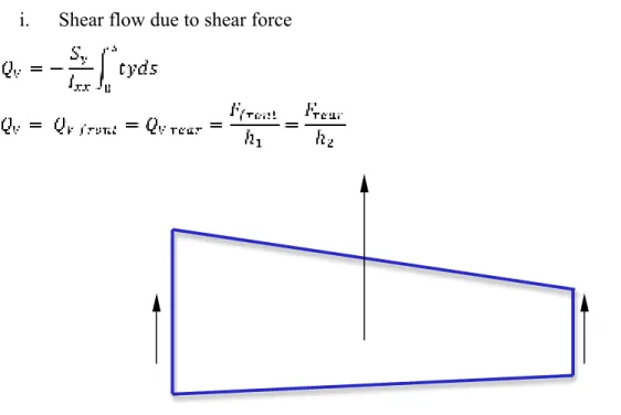
The criteria used for the front and rear spar is the same, so, for the thickness approach is also quite the same as follows. The spars are dimensioned by the shear flows. Actually, there are two sources of them:
i. Shear flow due to shear force
Figure 25 - Shear force applied in the wingbox
ii. Shear flow due to torsion force (equation 67)
Although, the senses of the shear flow due to torsion force are different for the front and rear spar, so, the total flow becomes:
As a result, the shear stress is:
50 Through the criteria and the critical shear buckling stress, with , = 5.4 and
, the thickness equation for the front and rear spar are below.
Finally, the equations for the thickness of each part of the wingbox are ready. So now, giving the input parameters to create the airfoil, the thickness of the upper skin, lower skin, front spar and rear spar of the entire wing are found. Then, the wingbox mass is calculated as follows.
In the next chapter, a wingbox analysis is made in order to choose the more adequate airfoils to study, not only for the analytical approach, but also for the numerical approach, made in reference [16].
2.7 Wingbox Analysis
The analytical approach is ready and the goal now is to find the regions that the program can build light wings, without compromising the wing geometry and aerodynamic effects as well, such as the drag force.
The NACA 4-digit airfoils have three parameters, being the input variables for the wingbox construction. For an analysis, it can have 7 cases:
i. Fix two parameters and vary the third one (3 cases). ii. Fix one parameter and vary the two others (3 cases). iii. Vary the three parameters at same time.
First of all, it is presented the cases of fixing two parameters, and the purpose is to discover the limitations of each variable and their sensibilities.
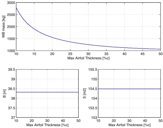
i. Case 1 – NACA 24XX, with XX = 10 to 50 ii. Case 2 – NACA 2X20, with X = 1 to 6 iii. Case 3 – NACA X420, with X = 1 to 9
So, for all them, the following graphics show the distribution of wingbox mass, the wingspan and the wing area, with the objective of understand the behavior of each parameter and so, catch the cases which the airplane has reasonable wing geometry and, if possible, the lightest weight as possible.
When the variation of maximum thickness is performed in case 1, it is detected that the wing geometry does not change, although the wing mass is modified. The reason for that consists in the fact of the lift generated by two NACA 4-digits airfoils with different maximum thickness is the same. But the change of maximum thickness also modifies the moment of inertia, then the efforts in the structure are not the same, as a result, the wing thickness is different, consequently, the mass as well.
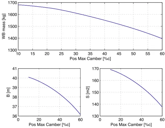
The cases 2 and 3 have the variation of wing geometry as expected. In relation with the wingbox mass, in one hand, the case 2 does not presents a huge variation of mass with the
52 variation of the position of maximum camber. In the other hand, the case 3 has a parabolic behavior, although it also not changes a lot in terms of mass.
10 15 20 25 30 35 40 45 50 1000 1500 2000 2500 3000
Max Airfoil Thickness [%c]
WB mass [kg] 10 20 30 40 50 37 37.5 38 38.5 39 39.5
Max Airfoil Thickness [%c]
B [m] 10 20 30 40 50 153 153.5 154 154.5 155 155.5
Max Airfoil Thickness [%c]
S [m2]
10 15 20 25 30 35 40 45 50 55 60 1300 1400 1500 1600 1700
Pos Max Camber [%c]
WB mass [kg] 0 20 40 60 36 37 38 39 40 41
Pos Max Camber [%c]
B [m] 0 20 40 60 130 140 150 160 170
Pos Max Camber [%c]
S [m2]
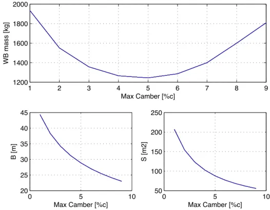
54 1 2 3 4 5 6 7 8 9 1200 1400 1600 1800 2000 Max Camber [%c] WB mass [kg] 0 5 10 20 25 30 35 40 45 Max Camber [%c] B [m] 0 5 10 50 100 150 200 250 Max Camber [%c] S [m2]
Figure 28 - Wingbox mass, wing span and wing area of the NACA X420, with X=1 to 9 (Case 3)
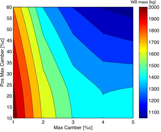
After analyzing these cases, the variation of two parameters have also a great relevance in order to achieve coherent conclusions and help in the decision of a few airfoils to be optimized in the numerical approach [16]. So, the variations chosen here are:
i. Case 4 – NACA 2XYY, with X = 1 to 6 and YY = 10 to 50 ii. Case 5 – NACA XY20
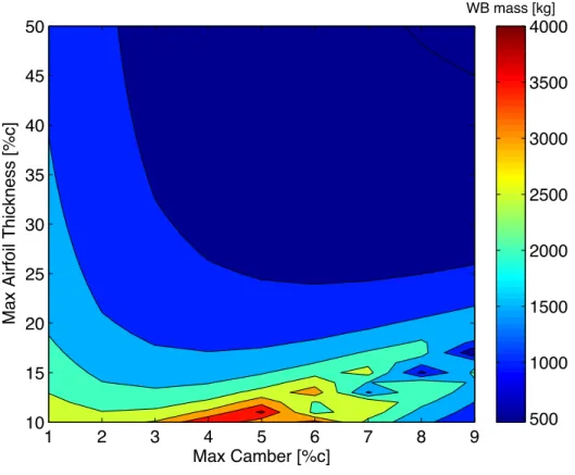
a. with X = 1 to 9 and Y = 1 to 6 b. with X = 1 to 5 and Y = 1 to 6 iii. Case 6 – NACA X4YY
a. with X = 1 to 9 and YY = 10 to 50 b. with X = 1 to 4 and YY = 10 to 50
Pos Max Camber [%c]
Max Airfoil Thickness [%c]
10 20 30 40 50 60 10 15 20 25 30 35 40 45 50 WB mass [kg] 1000 1200 1400 1600 1800 2000 2200 2400 2600 2800 3000
56
Max Camber [%c]
Pos Max Camber [%c]
1 2 3 4 5 6 7 8 9 10 15 20 25 30 35 40 45 50 55 60 WB mass [kg] 1000 1500 2000 2500 3000 3500 4000 4500 5000
Figure 31 - Wingbox mass of the NACA XY20, with X=1 to 9 and Y=1 to 6 (Case 5a)
Max Camber [%c]
Pos Max Camber [%c]
1 2 3 4 5 10 15 20 25 30 35 40 45 50 55 60 WB mass [kg] 1100 1200 1300 1400 1500 1600 1700 1800 1900 2000
Max Camber [%c]
Max Airfoil Thickness [%c]
1 2 3 4 5 6 7 8 9 10 15 20 25 30 35 40 45 50 WB mass [kg] 500 1000 1500 2000 2500 3000 3500 4000
Figure 33 - Wingbox mass of the NACA X4YY, with X=1 to 9 and YY=10 to 50 (Case 6a)
Max Camber [%c]
Max Airfoil Thickness [%c]
1 1.5 2 2.5 3 3.5 4 10 15 20 25 30 35 40 45 50 WB mass [kg] 1000 1500 2000 2500 3000 3500
58 Through the cases 5 and 6, the appropriate range of the maximum camber is between 1 and 5 %c, where the wingbox mass stays at low level. But, the decision of range should also take the wing geometry in account. By the case 3, it is coherent to at least eliminate the maximum camber of 1%c.
For the limit of maximum thickness, all graphics show that more the value of this parameter is high, lighter is the wingbox, although, every aircraft in this category does not use an airfoil with a maximum thickness more than 40%c. Moreover, when the maximum thickness is very low, the wing mass becomes very excessive.
Finally, the position of maximum camber is not so influent in the output, so it is practically indifferent, then, the range adopted to the field study is between 40 and 60%c, more coherent with the maximum camber used.
Based on the previous analysis it was decided 9 NACA airfoils to be optimized. So then, the data obtained through the analytical approach are used in the reference [16] as inputs, and optimized numerically. From the airfoils chosen, graphics displaying the distribution of thickness were constructed, below some of them are exposed as examples and the others are in the appendix D.
i. NACA 2415 ii. NACA 2420 iii. NACA 2520 iv. NACA 2620 v. NACA 3415 vi. NACA 4410 vii. NACA 4415 viii. NACA 4420 ix. NACA 4430
Figure 35 - WB Thickness along the wing for the NACA 2415
60
Figure 37 - WB Thickness along the wing for the NACA 3415
3.1 Theory/ Introduction
The surrogate model (response surface) is a tool that can replace a task that is taking too long time. In other words, if a process has inputs, a complex simulation and the output variables, an alternative is to approximate this fragment with a surrogate design. If it is well designed, it can run a lot of times very fast.
Figure 38 - Surrogate Model purpose
The surrogate models, also often referred as meta models, have a huge background with methods which supports and makes it valid. Then, of course, the final goal is to find an equation that gives the outputs by the insertion of inputs. The custom procedure passes by preliminary experiments, sampling plan (Design of Experiments), observations, then construct the surrogates, search infill criterion and, finally, add of new designs.
62
Figure 39 - Surrogate-based optimization framework [8]
Looking back to the surrogate framework, it should have started with preliminary experiments; however, the analytical approach and its analysis were already enough for that. For this reason, the wingbox is ready for the design of experiments. Then, after the sampling plan, it is the construction of the surrogate, where it should choose a function and later fit curves to make predictions. After that, the results must be verified with true points from the design due to the fact that surrogates are built upon assumptions. This step is called as infill points: a vital part of the process. This relevance comes from the need of validate the surrogate and proof the accuracy as well.
The quality of a surrogate is totally related with the information and assumptions made. Therefore, the success of that is obtained if the assumptions are well founded and if the information is correctly chosen. For now, there are two assumptions that are normally taken for a lot of surrogates: the engineering function is continuous and smooth.
Obviously, the idea is to have the most precise results as possible. The attempted of model perfection in all field of study is extremely hard, so then, the usual is to make predictions and then improve the results in the region of the optimum (the points of major interest), acquiring more correct answers there.
3.2 Design of Experiments (DoE)
Before constructing a surrogate model, the analysis through the design of experiments (DoE) can save cost and time. It is a method that deals with the selection and ordering of tests in order of immediately identify the parameter’s effects into the response surface.
Design of experiments has three phases:
i. Define a system comportment model (the coefficients can be unknown) ii. Define the DoE, creating series of tests for model coefficients identification iii. Do the tests, identify the coefficients and analyze the results
The goal of this section is to classify the relevance of each parameter in the outputs, and, if possible, eliminate some input variables. For now, the input variables for the surrogate model are:
i. Maximum Camber
ii. Position of Maximum Camber iii. Maximum Thickness
iv. Wing Station
The first three variables are functions of which airfoil it is used. The last variable, wing station, is a dependency of which part of the wing it is the thickness optimization. For the surrogate output, it has actually four: the Thickness of Upper Skin, Lower Skin, Front Spar and Rear Spar. However, they are treated individually, for the reason that one variable can be relevant for one output but not for the others, and so on.
In the aim of start the design of experiments, it should define the factors and levels for each one. The factors had already been chosen; they are the input variables, for their levels there are plenty of forms of doing that. A reasonable way is to define low (1), medium (2) and high (3) level. After that, it has to choose what values are going to be the levels for each factor. According to the chapter 2.1, in theory, the range for the NACA four-digits parameters is:
i. Maximum Camber: 0 to 9
ii. Position of Maximum Camber: 0 to 99 iii. Maximum Thickness: 0 to 99
64 Although, it is obvious that it should not go so far. A simple example of that is an airfoil that have maximum airfoil thickness of 90% of the chord would represent a wing of an extremely high drag, not the purpose to optimize it, as a result it ought to respect a minimum of aerodynamics effects.
It is also clear that the range is more restrict since it should has a compromise with the airplane characteristics, as already mentioned in chapter 2.1, a different airfoil implies in a different wing. Coming back to the chapter 2.7, it has analysis showing that influence, and as concluded there, some NACA parameters are impracticable, such as the NACA 1412, which outcomes a wing span of 40 m and a wing area of 200 m2, not usual values for the narrow-body commercial airliner.
For the range of the wing station, the idea is to take most part of the wing, the wing geometry was designed with 29 ribs equally spaced (following the chapter 2.1), hence it has 28 stations, named from the root to the wing tip. Taking into account all that, the following table shows the levels chosen for this study.
Table 10 - Input variables levels
Low Medium High
Maximum Camber 2 3 5
Position of Maximum Camber 30 40 50
Maximum Thickness 10 25 40
Wing Station 5 15 25
The next step is to specify the comportment model of the system, which is the mathematical relation that gives answer of the function by the factors and maybe others. It is supposed that the answer is just a function of the factors, so then:
Among the models with or without interactions between the factors, the model chosen is:
After that, to define the tests it should keep in mind the efficiency and robustness of the design of experiments. Consequently, Taguchi’s table is a good option, since it is a reduced model and thus, likely suitable for this study. The table is showed in Appendix E, in summary, this Taguchi’s table needs just 27 tests, that four factors with 3 levels would need 81 tests for a complete model.
Afterwards, the tests are done and it is time to identify the effects of each factor and the interactions. Through a Matlab code the factors’ influences are determined and easily visualized by the figures below. Just to remember, there is a design of experiment for each output (Thickness of Upper Skin, Lower Skin, Front Spar and Rear Spar); therefore a GUI interface was developed in Matlab for that. In this GUI, it is possible to change the levels for each factor and choose which output the user wants to analyze.
Figure 40 - Design of Experiments GUI
Consequently, using the interface explained above, the results for each output are quickly obtained. To begin with the experiments, the figures below only show the main’s variable influence.
66 1 1.5 2 2.5 3 3.5 4 4.5 Thickness(mm)
Max Camber (x1) Pos Max Camber (x2) Max thickness (x3) Section (x4)
Figure 41 - Main Variables’ influence in the Upper Skin
0 2 4 6 8 10 12 14 Thickness(mm)
Max Camber (x1) Pos Max Camber (x2) Max thickness (x3) Section (x4)
0.8 1 1.2 1.4 1.6 1.8 2 2.2 2.4 2.6 Thickness(mm)
Max Camber (x1) Pos Max Camber (x2) Max thickness (x3) Section (x4)
Figure 43 - Main Variables’ influence in the Front Spar
0.8 1 1.2 1.4 1.6 1.8 2 2.2 2.4 2.6 Thickness(mm)
Max Camber (x1) Pos Max Camber (x2) Max thickness (x3) Section (x4)
68 Throughout these graphics, it is evident for all cases that the position of maximum camber is not so influent in the thickness of the WB. As a consequence, there is a high probability of eliminating this input, although, it is important to see if the association of that variable with another one is relevant or even other coupled cases that are not evident to see just by these graphics. For that, the following figures show all these parameters. Before analyzing these figures, the table 12 summarizes the previous figures about the main variables’ influence, which allows a global view of this segment.
Table 11 - Main Variables' influence
Max Camber Pos Max Camber Max thickness Section
Upper Skin Low Very Low Medium High
Lower Skin Medium Very Low High High
Front Spar Low Very Low Medium High
Rear Spar Low Very Low Medium High
1 1.5 2 2.5 3 3.5 4 4.5 Thickness(mm) Max Camber (x1) Pos Max Camber (x2) x1x2 x1x22 Max thickness (x3) x1x3 x1x32 x2x3 Section (x4) x2x32
0 2 4 6 8 10 12 14 Thickness(mm) Max Camber (x1) Pos Max Camber (x2) x1x2 x1x22 Max thickness (x3) x1x3 x1x32 x2x3 Section (x4) x2x32
Figure 46 - Variable's influence in the Lower Skin
0.8 1 1.2 1.4 1.6 1.8 2 2.2 2.4 2.6 Thickness(mm) Max Camber (x1) Pos Max Camber (x2) x1x2 x1x22 Max thickness (x3) x1x3 x1x32 x2x3 Section (x4) x2x32
70 0.8 1 1.2 1.4 1.6 1.8 2 2.2 2.4 2.6 Thickness(mm) Max Camber (x1) Pos Max Camber (x2) x1x2 x1x22 Max thickness (x3) x1x3 x1x32 x2x3 Section (x4) x2x32
Figure 48 - Variable's influence in the Rear Spar
Investigating all pictures at same time, the coupled factors have not a great influence compared to the pure factors; nevertheless there are still influences that can produce little differences. Particularly, the coupled case x1x2 (Max Camber with Position Max Camber) is a bit more critical than the variable Max Camber alone, excepting the Upper Skin output.
In engineering, it should always keep in mind the compromise between time and accuracy. Wherefore, based on these graphics, it is reasonable to exclude the variable position of maximum camber without prejudging the accuracy of results. Furthermore, for now, designing a surrogate model with three variables will be faster to build up and also control future results. Moreover, with the same variables for all parts of the wingbox, it should only make one response surface for all them, that gives the 4 outputs at once (Upper Skin, Lower Skin, Front Spar and Rear Spar thickness).
3.3 Surrogate Model
After the analysis of the design of experiments it is time to construct the surrogates. Actually, for this project it is possible to build up response surface for the analytical approach and also for the numerical approach.
In the case of the analytical approach, made in the first part of this project, the surrogate model will find the analytical outputs by the insertion of the desired inputs. Remembering that the analytical outputs are also the inputs for the numerical analysis in NASTRAN, so they can also be seen from this point of view. For the numerical approach, the concept is quite the same except from the fact that the points of data are different and more restrict, being more difficult to achieve good results.
A. Surrogate Model for the Analytical approach results
Through a MATLAB code, the response surface for the analytical results of the wingbox is made following the steps explained in the section 3.1. First, the bounds are fixed for each parameter.
i. Maximum thickness: 10 to 40 %c ii. Section: 2 to 28
iii. Maximum camber: 2 to 6 %c
Then, it must choose the cases that will be part of the surrogate construction. For that, the Box-Behnken has been selected, which is a MATLAB tool that takes the minimum, medium or maximum value of each variable, composing 15 events (Appendix E). Actually, it takes the midpoints of edges of the design space and also the center that is taken three times for a more uniform estimation of the prediction variance. This tool has the advantage of being fast, although it has poor results around the extremes.
72
Figure 49 - Geometry of a Box-Behnken design [20]
After that, the wingbox is calculated for each point of the Box-Behnken design with the MATLAB code from the analytical approach. Therefore, by choosing the model, the fitted functions are obtained and then, the infill points verify the quality of the surrogate raised. It was decided to use the full quadratic model for all the parts of the wingbox.
15 20 25 30 35 1 2 3 4 5 −20 0 20 40 1 2 3 0.5 1 1.5 2 2.5 5 10 15 20 25 2.5 3 3.5 4 4.5 5 5.5
Figure 50 – Slices of the Response Surface of each part of the wingbox
Through the MATLAB code, the coefficients of the model were determined and also the root mean square error (RMSE), which indicates the quality of the regression function, since it measures the disparities between the prediction points and the true points. More the RMSE is near to zero, more precise is the model design.
Table 12 - Reduced Model Coefficients for each part of the WB
Upper Skin Lower Skin Front Spar Rear Spar
B0 8.220 40.092 4.132 4.709 B1 -0.109 -2.494 -0.077 -0.088 B2 -0.170 -1.545 -0.066 -0.072 B3 -0.481 8.052 -0.136 -0.170 B4 0.002 0.052 0.001 0.001 B5 0.004 -0.202 0.001 0.001 B6 0.008 -0.055 0.002 0.003 B7 0.001 0.037 0.001 0.001 B8 -0.002 -0.005 -0.001 -0.002 B9 0.015 -0.016 0.006 0.007
Table 13 - Root Mean Square Error of each part of the WB
Upper Skin Lower Skin Front Spar Rear Spar
RMSE 0.1146 6.0291 0.103 0.0926
From the RMSE table above, it is clearly evident that the lower skin prediction has low worth beyond the others surrogates. As a result, poor results are acquired for the lower skin. In order to find the reason for that, the analytical approach section shows that the distribution of thickness in the wing for the lower skin is more unpredictable and also has a great difference between the maximum and minimum value of thickness. Moreover, the lower skin distribution of thickness changes a lot for each airfoil, which turns the modeling more complicated than the others.
Consequently, from now on, the parts of the wingbox analyzed are just the upper skin, front spar and rear spar. Actually, it is not so serious the elimination of the lower skin, because in the industry, the lower skin is not usually dimensioned with the stress criteria, but they use fatigue criteria as the main factor. Furthermore, the numerical optimization [16] confirms that the stress a criterion is not used for the lower skin, so the results exposed are just for the others parts.
After building the surrogate model, it should be validated. For that, it was taken the NACA airfoils that were already mentioned in the wingbox analysis (section 2.7) and used in the numerical optimization. Comparing the surrogate models with these airfoils, the relative errors are showed below along the wingspan for the upper skin, front spar e rear spar, respectively.
74
Figure 51 - Relative Error distribution for the Upper Skin Surrogate Model
Figure 53 - Relative Error distribution for the Rear Spar Surrogate Model
From the three graphics above, the errors are more than 10% in some parts; so, it needs a solution to fix it. Looking at the behavior of the relative errors, the two major critical points are around the engine position (near of the 10th section) and also at the end of the wing (around the 25th section). The engine position is clearly a problem, since it inserts a discontinuity at the distributions, and then, it is harder to design just one surrogate for both parts (before and after the engine). The problematic at the end of the wing is that around the 25th section, the thickness for all parts of the wingbox achieve 1mm (the minimum thickness adopted), as a result, the reduced model does not follows that behavior, increasing the errors nearby that region.
Although the simplicity of doing only one surrogate for each part of the WB, the precision for some portions are far from reasonable values. Thus, one idea is to make more than one surrogate. For the upper skin response surface, it is probably enough to make 2 surrogates, but for the front and rear spar, it is more prudent to build up a surrogate before the engine position, another one between the engine position and the 25th section, and the third after the 25th section. The following figure shows the new results of the upper skin surrogate model, making 2 response surfaces:
i. 1st to 20th section: Full Quadratic function ii. 20th to 28th section: Linear function
76
Figure 54 - Relative Error for the Upper Skin with 2 surrogate models
Comparing this result with the previous upper skin response surface, this one has lower relative errors, which indicates that the choice of design space directly affects the quality of answers, and that, for this case, is better to separate into two design spaces and build up two surrogate models for the upper skin.
B. Surrogate Model of the Numerical WB results
The modeling of the response surface for the numerical WB results is the quite same as used for the surrogate of the analytical results. The only differences are the selections of points and the reduced model used. About the selection of points, this time it comes from the NACA airfoils used in the numerical optimization (8 airfoils), instead of the Box-Behnken used before. And for the reduced model the fitted function used is interactions, since the quantity of points is not so high. The function is showed as follows.
Between the 8 NACA airfoils used in the numerical results [16], one of them should stay outside the points of surrogate construction to be, afterwards, the infill points. At this way, it is possible to build up 8 surrogates, and then they can be compared and analyzed. For example, the surrogate 1 uses the 8 NACA airfoils except the NACA 2415, and then, that one will be used as infill points, for the response surface validation. The table below shows the RMSE for each surrogate model.
![Figure 15 - Loads creates by the elliptic lift distribution in the wing [4]](https://thumb-eu.123doks.com/thumbv2/123doknet/2357728.38365/33.892.217.721.127.757/figure-loads-creates-elliptic-lift-distribution-wing.webp)