HAL Id: hal-03193898
https://hal.archives-ouvertes.fr/hal-03193898
Submitted on 9 Apr 2021
HAL is a multi-disciplinary open access
archive for the deposit and dissemination of
sci-entific research documents, whether they are
pub-lished or not. The documents may come from
teaching and research institutions in France or
abroad, or from public or private research centers.
L’archive ouverte pluridisciplinaire HAL, est
destinée au dépôt et à la diffusion de documents
scientifiques de niveau recherche, publiés ou non,
émanant des établissements d’enseignement et de
recherche français ou étrangers, des laboratoires
publics ou privés.
Ecole Temps Réel 2017 - Uniprocessor real-time
scheduling
Julien Forget
To cite this version:
Julien Forget. Ecole Temps Réel 2017 - Uniprocessor real-time scheduling. Doctoral. France. 2017.
�hal-03193898�
´
Ecole Temps R´eel 2017
Uniprocessor real-time scheduling
Julien Forget
Univ. Lille, France Email: [email protected]
Abstract—A real-time system is a computer system where it is just as important to compute a correct value as it is to compute this value at the right time. Such a system is usually modelled as a set of tasks that must satisfy real-time constraints (periods and deadlines mainly). Real-time scheduling consists in finding a task execution order that satisfies all real-time constraints.
In this paper, we provide a brief overview of real-time schedul-ing on uniprocessor systems. We present classic schedulschedul-ing policies and associated schedulability analyses. In addition, the paper gives some background on the relation between the classic real-time task model and dynamics of the modelled system. It also emphasizes the role of data-dependencies, how they are implemented and their impact on scheduling. [1], [2] have been great sources of inspiration for this paper.
I. INTRODUCTION
A real-time system is a computer system subject to a set of real-time constraints: not only does such a system need to compute the correct values, it must do so in a timely manner. For instance, let us consider the longitudinal flight control system of an airplane, such as [3]. This system controls the angle of the control surfaces of the plane based on the current state of the plane and on the altitude required by the pilot. An important real-constraint is that the time required for the system to adjust the control surfaces in reaction to a pilot order or to a gust of wind must respect a predefined delay, in order to ensure the plane stability. Similar constraints can be found in many other areas, such as for instance in assisted driving systems in the automotive domain, in nuclear plant surveillance systems, in video processing systems, ...
A real-time system is usually modelled as a set of tasks, each with its own dedicated functionality and real-time con-straints. Real-time scheduling consists in finding an execution order for tasks, which satisfies all the task real-time con-straints. This is a twofold problem. On one hand, we must choose a scheduling policy capable of satisfying the real-time constraints. General purpose scheduling policies (FIFO, Round-Robin, etc) are not well-adapted to real-time systems, since they usually focus on reducing the average response time of processes. In a real-time system, what matters is that tasks respect their real-time constraints in the worst-case. On the other hand, real-time systems are usually critical, so developers need a schedulability analysis, which ensures before execution that, for a given scheduling policy, the resulting execution will always respect the system real-time constraints.
In this paper, we focus on the scheduling of systems executing on a single computation core. The paper first details the classic way to model a real-time system (Section II). In addition to providing usual definitions on task real-time char-acteristics, it tries to relate these constraints to the dynamics of the system, and also gives a brief overview on how real-time tasks are usually implemented. Though the classic real-time task model assumes independent tasks, tasks are actually often related by data-dependencies. Section III discusses the mod-eling and implementation of such dependencies. Scheduling terminology and problem definition are provided in Section IV. Main results on uniprocessor schedulability analysis are pro-vided in Section V, for fixed-task priority scheduling, and in Section VI, for fixed-job priority scheduling. Scheduling of dependent tasks is presented in Section VII.
II. REAL-TIME TASKS
Real-time systems can be separated into two sub-classes: event-driven systems and sampled systems. In an event-driven system, the system waits for an input event to occur and then computes its reaction. In a sampled system, the system acquires its inputs at regular intervals of time and computes its reaction for each sample of its inputs. While the event-driven model is potentially more expressive, sampled sys-tems are usually easier to analyze and their behaviour is more predictable, especially concerning the real-time aspects. Furthermore, in many event-driven systems, the time that separates the occurrence of two events can be lower-bounded, in which case the scheduling problem becomes quite similar to that of sampled systems (see sporadic tasks below). A. Real-time constraints
a) Period: A periodic task executes at regular intervals of time, as defined by its period. The period of a task is chosen as follows. On one hand, the period of a task must be below some bound, related to the inertia and physical characteristics of the device it controls. Above this value, the safety of the device (e.g. the stability of the airplane) is not ensured. This bound differs between the different physical devices of the controlled system. For instance, the propulsion devices of a space vehicle must be controlled very fast to ensure the stability of the vehicle, while the position of its solar panels can be controlled a little slower as a little energy loss has less dramatic impact on the vehicle. On the other hand, the period
must be above some bound, below which the device will not be able to apply the commands fast enough or may get damaged. Of course, this lower bound also differs from one device to another. The period is usually chosen as close to the upper bound as possible, which spares unnecessary computations and thus enables the use of less powerful hardware, reduces energy consumption, and so on.
b) Deadline: The deadline of a task bounds the maxi-mum time allowed between the task invocation and the task completion. In many real-time systems, it is equal to the task period, meaning that one invocation of a task must complete before the next invocation of that task. In some systems, the deadline can be lower than the period. While this may, in rare cases, correspond to a constraint related to the system dynamics, in most cases it is used as a way to artificially influence the system schedule, because tasks with shorter deadlines will usually be scheduled first (see scheduling techniques for dependent tasks in Section VII for instance). Systems where the deadline of a task can be higher than its period are quite uncommon, though they have been studied in the literature.
c) Offset: In some systems, offsets are associated to tasks. Instead of releasing tasks simultaneously at system start-up, tasks are released at the date specified by their offset. This parameter is rarely related to the system dynamics but rather to implementation concerns (again, see Section VII for instance). d) WCET: Performing a schedulability analysis requires the knowledge of the execution time of each task. Since the exact execution time of a task can be very hard to predict, an approximate worst-case execution time (WCET) is usually considered. It is pessimistic, in the sense that actual execution time might be lower, but safe, in the sense that the actual execution time will definitely be lower. WCET is not a real-time constraint per se, since we do not need to force a task to execute for as long as its WCET. It is nonetheless essential for system analysis.
e) Task model: We will use the following notations. A real-time task is denoted τi(Ci, Ti, DiOi), where Ci is the
WCET of τi, Ti is its activation period, Di is its relative
deadline and Oi its offset. In this paper, we assume that
Di ≤ Ti and Oi ≥ 0, though more commonly it is assumed
that Di = Ti and Oi= 0.
We denote τi.kthe kth(k ≥ 0) invocation, or job, of τi. For
periodic tasks, the job τi.k is released at time oi.k= Oi+ kTi.
For sporadic tasks, we have oi.k≥ Oi+ kTi instead. In both
models, every job τi.k must be completed before its absolute
deadline di.k= oi.k+ Di. In the following, we will focus on
periodic tasks. The hyperperiod of a task set, which we will denote HP , is defined as the least common multiple of the periods of the tasks.
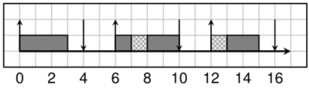
Figure 1 illustrates task real-time parameters for a periodic task τi(3, 6, 4, 0). Gray rectangles correspond to the execution
of τi, while hatched rectangles correspond to time intervals
during which the system is busy executing another task. τi.1
is preempted after it starts its execution to execute another task (about preemption, see Section IV). τi.2executes for less than
0 2 4 6 8 10 12 14 16
Fig. 1. Execution of a real-time task
the WCET (2 instead of 3). The jobs all respect the deadline constraints.
B. Implementation
A real-time task is usually implemented using mechanisms akin to threads, provided by the (Real-Time) Operating Sys-tem. While the exact code is dependent on the target OS, the global structure remains more or less the same. Algorithm 1 details the typical implementation of a periodic task in pseudo-C code, while Algorithm 2 illustrates how to invoke such tasks. Concerning Algorithm 1:
1) The task first goes through an initialization phase and then waits for its initial release. In RTOS derived from Linux (for instance RTAI [4] or the ptask API [5]), tasks start executing as soon as they are created, just like threads. Since creating all the tasks takes time, the programmer needs to implement in this phase mecha-nisms that synchronize the initial release of tasks (e.g. a synchronization barrier). In other RTOS, such as FreeR-TOS for instance [6], tasks start only when the scheduler is explicitly invoked (start_schedulerin Algorithm 2),
so only tasks with offsets need to explicitly wait for the initial release;
2) Once the initialization phase is complete, the task starts executing periodically. It repeats indefinitely the same behaviour: 1) execute the code corresponding to the actual functionality of the task; 2) wait for the next task activation (typically, wait for the next period).
Concerning Algorithm 2:
• The task creation primitive usually takes, at least, three
parameters: 1) a pointer to the task function that defines the task functional behaviour (like periodic_task1); 2)
the arguments (often empty) to pass to that function (here, to functionperiodic_task1); 3) the real-time parameters
of the task;
• In a RTOS where tasks start executing as soon as they are created, we usually add an infinite idle loop (while(1);) at the end of themainfunction, because the termination of themainfunction causes the termination of the tasks. In other systems, the execution of tasks starts when the scheduler is explicitly invoked (start_scheduler). Even though the task structure presented here is very common, RTOS usually allow more complex task implemen-tations, where for instance the code executed by the task changes from one iteration to the next, where the period can be modified dynamically, etc. For instance, a common rookie mistake is to forget to wait for the next period at the end
of a task iteration. This is in no way verified by the OS or by the compiler, even though this causes obvious problems at execution. So, it is up to the programmer to ensure that the program respects the task model that was used to perform the schedulability analysis.
RTOS that follow the OSEK standard [7], including Tram-poline [8], opt for a more rigid approach where the task set and its real-time characteristics are defined statically in a dedicated OIL file [9]. The task implementation model is predefined and the user only provides the function corresponding to a single iteration of the task (the task_functionality() function in Algorithm 1), which is automatically repeated by the RTOS at each task invocation. This model is less permissive, but it prevents some design mistakes, such as those discussed earlier for instance (immediate loops or main function finishing and killing tasks).
Algorithm 1 Typical implementation of a periodic task
void* periodic_task1(void* args) {
//initialization wait_for_release(); while (1) { task_functionality(); wait_next_activation(); } }
Algorithm 2 Typical program for invoking two tasks
int main() {
// initialize real-time parameters params1 create_task(periodic_task1,args1,params1); // initialize real-time parameters params2 create_task(periodic_task2,args2,params2); // either start_scheduler(); or while(1); // This should never be reached
return 1; }
III. DATA-DEPENDENCIES
The seminal work on real-time scheduling of periodic tasks by Liu & Layland [10], and a very large portion of the real-time scheduling literature, assume real-time systems consisting of independent tasks, meaning that there is no a-priory ordering constraint relating tasks. Obviously though, tasks collaborate to compute the system outputs and as a result are related by data-dependencies, meaning that some tasks produce data used by some other tasks to perform their own computations.
A. Communication semantics
There are mainly two possible semantics for data-communications. With register-based communications, used
for instance in the automotive domain [11], when a task executes it consumes the last value produced, not considering when it was produced. With such communications, the relative order between the task producing the data and the task con-suming it remains unconstrained. On the contrary, with causal communications, the task producing the data must complete its execution before the task consuming it starts its execution. Such communications yield more deterministic systems and are thus preferred in critical systems, such as avionics systems for instance [3].
Causal communications introduce additional real-time con-straints, called precedence constraints: a precedence constraint requires one task to execute before another. A dependent task set is modelled as a directed acyclic task graph G = (S, E), where S = ({τi(Ci, Di, Ti, Oi)}1≤i≤n) is a set of tasks, as
defined previously, and E ⊆ S ×S. A precedence constraint, is denoted τi→ τj, with τi → τj ≡ (τi, τj) ∈ E. If Ti= Tj, we
say that τi→ τjis a simple precedence constraints. Otherwise
we say that it is an extended precedence constraint. B. Extended precedence constraints
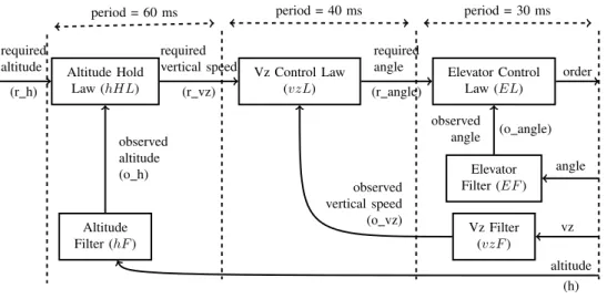
In the general case, precedence constraints may relate tasks with different periods. Such a system is illustrated in Figure 2, which describes the tasks of the longitudinal flight control system of an aircraft (this description is based on [12]). This system controls the angle of the control surface (order) based on: the current surface angle (angle), the current aircraft vertical speed (vz), the current aircraft altitude (altitude) and the altitude required by the pilot (required altitude). The software architecture consists of six tasks that make up three computation chains:
• A fast chain operating at 30 ms from EF to EL, which controls the control surface according to a required angle;
• A multi-rate chain from vzF (period 30 ms) to vzL (period
40 ms), then to EL (period 30 ms), which controls the vertical speed;
• A multi-rate chain from hF (period 60 ms), to hHL (period 60 ms), to vzL (period 40 ms), to EL (period 30 ms), which controls the trajectory the plane follows to reach the altitude ordered by the pilot.
An extended precedence constraint τi → τj(where Ti6= Tj)
only imposes precedence constraints on a subset of the jobs of τi and τj. The system model must thus specify the set of
pairs (p, q) such that τi.p→ τj.q.
In most real-time applications and design tools, such as Simulink [13], AADL [14] or Prelude [15] for instance, extended precedence constraints follow patterns repeated peri-odically on the tasks hyperperiod. Some examples of extended precedence constraints are illustrated in Figure 3 (see [16] for more details on extended precedence constraints models). The programmer can use the patterns of Figures 3(a), 3(b), to leave flexibility for the execution of the slow task: the slow task consumes values produced early, i.e. samples only the first out of 3 successive jobs of the producer, and produces values late, i.e. communicates with the last out of 3 successive jobs of
Altitude Hold Law (hHL) Altitude Filter (hF ) Vz Control Law (vzL) Elevator Control Law (EL) Elevator Filter (EF ) Vz Filter (vzF ) observed altitude (o h) required altitude (r h) required vertical speed (r vz) observed angle (o angle) observed vertical speed (o vz) required angle (r angle) order angle vz altitude (h)
period = 60 ms period = 40 ms period = 30 ms
Fig. 2. Vertical speed control τi τi τi τi τi τi
τj τj
(a) Sampling, at earliest
τi τi τj τj τj τj τj τj (b) Selection, at latest τi τi τi τi τi τi τj τj (c) Array gathering τi τi τjτj τj τjτj τj (d) Array scattering Fig. 3. Extended precedence constraints
the consumer. The patterns of Figure 3(c) and Figure 3(d) cor-respond to classic signal processing patterns, where repetitive array computations are distributed between several repetitions of the same task: on one hand the slow task scatters the content of a big array between successive jobs of its consumer and on the other hand it gathers array fragments from its producer to construct a big array. These two patterns behave in a fashion similar to the MPI_gatherandMPI_scatterprimitives of the popular Message Passing Interface (MPI) API [17].
IV. REAL-TIME SCHEDULING:PROBLEM DEFINITION
As mentioned earlier, scheduling real-time systems requires to:
1) Design a scheduling policy that will decide how to order the execution of tasks;
2) Design a schedulability test that will ensure, before sys-tem execution, that the execution order produced by the scheduling policy will respect the real-time constraints. A. Schedulability
The execution of a set of real-time tasks is controlled by a schedulerthat decides at each instant which task to execute on the processor. For a given schedule (produced by the chosen scheduler), we let e(τi.k) denote the start time of τi.k in the
schedule and s(τi.k) denote its completion time. The validity
of a schedule is established as follows:
Definition 1. A schedule is feasible if it respects the following constraints:
∀τi.p, s(τi.p) ≥ oi.p (1)
∀τi.p, e(τi.p) ≤ di.p (2)
∀τi.p→ τj.q, e(τi.p) ≤ s(τj.q) (3)
A scheduling policy is a set of rules that dictates how the scheduler will choose which task to execute. A task set is schedulable by a given scheduling policy if and only if the schedule it produces is feasible. A schedulability analysis checks whether a given task set is schedulable by a given scheduling policy. This analysis is usually performed statically, that is to say before system execution. Except for simplified problems, schedulability analysis is NP-hard. Therefore, exist-ing analyses are either exact and have exponential complexity, or are pessimistic and have a polynomial or pseudo-polynomial complexity. With a sufficient schedulability test, all task sets considered schedulable by the test are actually schedulable. With a necessary schedulability test, all task sets considered unschedulable by the test are in fact unschedulable. An exact test if both sufficient and necessary.
B. Scheduling policy classes
Scheduling policies can be separated in different classes of policies. A scheduling policy is preemptive if it allows interrupting a job during its execution and resuming it later (e.g. to execute a higher priority task). Off-line scheduling consists in computing a (cyclic) feasible schedule before system execution. In that case, the scheduler becomes a simple dispatcher that repeats indefinitely the off-line schedule during execution. With on-line scheduling, the scheduler computes the schedule as execution progresses, based on the chosen schedul-ing policy. Most on-line schedulschedul-ing policies are priority-based, meaning that they only define how to assign priorities to tasks and that the scheduler then always chooses to execute the highest priority ready task.
A scheduling policy P is optimal within a certain class of policies if the following holds: if a task set is schedulable by some policy of this class, then it is schedulable by P. For instance, we will see that the Deadline Monotonic policy is optimal within the class of fixed-task priority policies, for independent task sets without offsets. In this paper, we will focus on on-line priority based preemptive policies.
C. Fixed-tasks vs fixed-job priority policies
With a fixed-task priority scheduling policy (FTP), the priority of a task remains unchanged during the whole sys-tem execution. It is the most widely used class of policies for scheduling real-time systems and every RTOS provides support for it. With a fixed-job priority scheduling policy (FJP), the priority can differ between jobs of the same task, but remains unchanged for a given job. Liu and Layland [10] proposed the rate-monotonic (RM) fixed-task priority policy, where tasks with a shorter period are affected a higher priority and the earliest-deadline-first (EDF) fixed-job priority policy, where jobs with a shorter absolute deadline are affected a higher priority. RM is optimal within the class of fixed-task priority policies for periodic task sets with Ti = Di and
Oi= 0. It can be extended to the deadline-monotonic policy
(DM) [18], to schedule optimally a set of tasks with Di ≤ Ti
and Oi= 0. For the case where Oi≥ 0, an optimal algorithm
based on DM was defined by Audsley in [19]. EDF is optimal in the class of fixed-job priority policies for scheduling a set of periodic tasks with Di≤ Ti and Oi≥ 0.
RM tends to be favored instead of EDF by real-time devel-opers, at least for uniprocessor systems. A detailed comparison is available in [20], it can be summarized as follows:
• Implementation: With FTP, task priorities can be com-puted before run-time (either by the programmer or at start-up by the OS), while with FJP they must be computed by the scheduler at run-time, each time a task is released. Furthermore, RTOS always provide support for fixed-task priority scheduling, while it is not always the case for fixed-job priority scheduling;
• Run-time overhead: FJP requires to compute task priori-ties at run-time, which introduces a run-time overhead that does not exist with FTP. However, when context switches are taken into account, FJP introduces less overhead than FTP because the number of preemptions that occur with FJP is usually much lower than with FTP;
• Task jitter: The task jitter is the variation between the
response times of different jobs of the task. FTP reduces the jitter of high priority tasks but increases that of low priority tasks, while FJP treats tasks more equally. As a result, when the utilization factor of the processor is high (i.e. when the processor has few idle times), the average task jitter of the task set is lower with FJP than with FTP;
• Overloads: When the total execution time demand of tasks exceeds the processor capacity, FTP causes less deadline misses than FJP. The problem with FJP is that if a task misses its deadline and carries on anyway, it causes other tasks to miss their deadlines (domino effect);
• Processor utilization: FJP enables better processor
uti-lization (up to 100%) than FTP (around 70-80%), thus allowing more complex computations to be performed. V. SCHEDULABILITY WITHFIXED-TASK PRIORITY
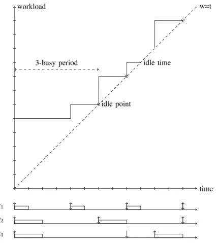
A. Busy period
The concept of busy period plays a central role in the schedulability analysis of FTP. A k-busy period is a time interval where the processor is kept busy executing task of priority higher than or equal to k. This is illustrated in Figure 4. The step function corresponds to the cumulative demand for execution on the processor, also called the Demand Function. At time 0, three jobs are released so the Demand Function steps for an amount equal to the sum of the three jobs WCET. This starts the first 3 − busy period of the system. This period finishes when the Demand Function meets the Time Function w = t (at time t, the processor has executed t units of work). Such a meeting point is called an idle time: the processor remains idle until the next job release.
The response-time of a job is the time interval from the job release to the job completion. The worst-case response-time of a task is the greatest response-time of its jobs. A task-set is schedulable if and only the worst-case response-time of each task is lower than its deadline. The following theorem enables to relate response times to busy periods
Theorem 1 ([19], [21]). The worst-case response time of a task of priorityk is equal to the longest k−busy period.
So, to check system schedulability, we can compute the longest k-busy period of each task τk and compare it to its
deadline. A busy period always ends on the condition that the processor utilization ratio U = Pn
i=1 Ci
Ti ≤ 1 (note that this
is also a trivial necessary schedulability condition for FTP). In other words, if this condition is fulfilled, then there is at least one idle time. Let n be the lowest priority of the system, if U = 1 then the length of the longest n−busy period is equal to the hyperperiod of the task set (HP ). Since HP is the least common multiple of the periods of the task set, HP is exponential with respect to the number of tasks of the task set.
In [22], authors propose a pseudo-polynomial solution for computing the length of the longest i−busy period Bi. It is
computed as the least fixed-point of the following equation (where hp(i) denotes the tasks with higher priority than τi):
Bi,0= Ci Bi,k+1= Ci+ X j∈hp(i) dBi,k Ti eCj B. Schedulability tests
Response-time analysis (RTA) based on the busy period, as presented in the previous section, provides a feasibility test that is actually independent of the scheduling policy. Indeed, since it is a necessary and sufficient schedulability condition, then any optimal scheduling policy can rely on
time workload w=t ◦ idle point ◦ idle time ◦ 3-busy period τ1 τ2 τ3
Fig. 4. Time demand function
this condition. Unfortunately, RTA does not have polynomial complexity. In this section we discuss some less complex specific schedulability tests.
For RM, the following sufficient schedulability test was proposed in [10]:
U = n(21/n− 1)
It is however quite pessimistic. It yields maximum processor utilization ratios between 80% (for smaller values n) and 70% (for greater values of n), while simulations show that the average bound is around 88% [23]. Tighter utilization bound tests have been proposed in [24], [25].
For DM, exact exponential schedulability tests have been proposed in [26], [27].
Le us now consider systems with offsets. A critical instant occurs when all the tasks are released simultaneously. It was proved in [19] that the longest busy period is initiated by the critical instant. For systems without offsets, this means at date 0. For systems with offsets however, the critical instant may not exist, which means that we need to study all the busy periods up to max(Oi) + 2HP [18], [28].
C. Shared resources
Using mutual exclusion mechanisms to handle shared re-sources in real-time application scheduled with FTP, via either
mutexes or semaphores, introduces two well-known sources of bugs: priority inversion and scheduling anomalies.
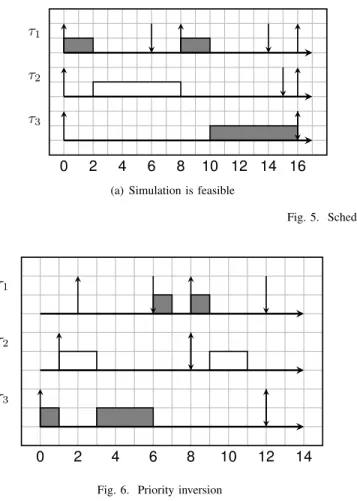
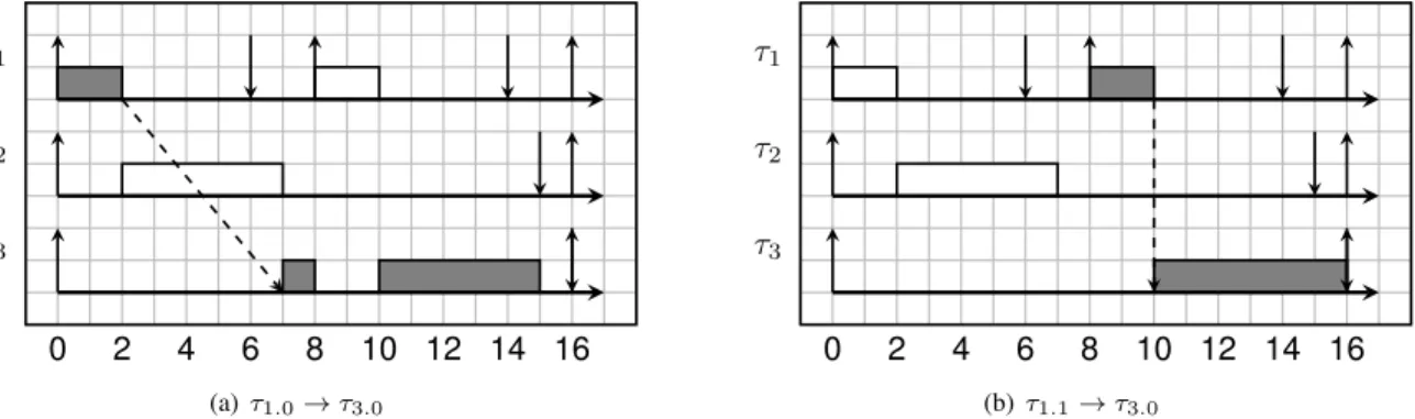
A scheduling anomaly occurs when the system is deemed schedulable by a schedulability test, but the schedule produced at execution is infeasible, due to a task executing for less than its WCET. This is illustrated in Figure 5. We consider a task set without offsets S = {τ1(2, 8, 6), τ2(6, 16, 15), τ3(6, 16, 16)}
where tasks sharing a resource using mutexes are depicted in gray. When C2 = 6, the schedule is feasible, while it is not
when C2 = 5 (τ1 misses its deadline). This phenomenon is
quite counter-intuitive, since here reducing an execution time produces a worse case. This implies that we cannot rely on a simple simulation to test the feasibility of a task set with shared resources.
A priority inversion occurs when a task is delayed by a lower priority task, even though it does not share a resource with it. This is illustrated in Figure 6. We consider a task set with offsets, where mutual exclusion sections are depicted in gray. In this example, τ2 is running while the highest priority
task τ1is waiting for τ3 to complete its critical section, which
causes τ1 to miss its deadline.
An intuitive solution to prevent priority inversion is the Priority Inheritance Protocol (PIP) [29]: when a task gains control of a shared resource, it inherits the priority of the highest priority task that shares this resource, until completion of its critical section. This completely prevents priority
inver-0 2 4 6 8 10 12 14 16 τ1
τ2
τ3
(a) Simulation is feasible
0 2 4 6 8 10 12 14 16 τ1
τ2
τ3
(b) Execution is infeasible Fig. 5. Scheduling anomaly
0 2 4 6 8 10 12 14 τ1
τ2
τ3
Fig. 6. Priority inversion
sions, however the number of times a task can be blocked when trying to enter its critical section can be quite high. Authors of [29] instead proposed the Priority Ceiling Protocol (IPCP, here we consider the “immediate” variation of the protocol), which reduces blocking times. Each resource has a priority ceiling equal to the highest priority amongst task using it. When a task executes, its priority becomes the maximum of the priority ceilings of the resources it uses. As a consequence, a task can only be blocked once, at the beginning of its execution. Indeed, to start executing all the resources it requires must be free, otherwise it is blocked (by higher priority tasks). IPCP is readily available in many real-time executives (e.g. Real-Time POSIX, OSEK/VDX, Real-Time Java).
VI. SCHEDULABILITY WITHFIXED-JOB PRIORITY
A. Schedulability tests
When Di = Ti and Oi = 0, schedulability with EDF is a
very simple problem: it was proved in [10] that U ≤ 1 is an exact schedulability condition.
When Di ≤ Ti and Oi = 0, the problem becomes much
more difficult. Unfortunately, the worst-case response time does not occur at a critical instant, which makes response-time analysis for EDF quite difficult. Instead, schedulability tests for EDF rely on the concept of processor demand [30]. The processor demand h(t), which represents the amount of
work that must be completed before time t, can be computed as follows: h(t) = n X i=1 bt + Ti− Di Ti cCi
As the load must never exceed the available processing time, schedulability can be stated as:
∀t, h(t) ≤ t
Schedulability analysis checks this condition on a limited number of values of t, by noting that: 1) h(t) only increases at job deadlines; 2) there exists an upper bound L on the values of t that must be checked. Two formulas have been provided to compute L. The first bound La is computed as follows:
La = max{D1, . . . , Dn,
Pn
i=1(Ti− Di)Ci/Ti
1 − U } The second bound Lbis the least fixed-point of the
follow-ing recurrence: w0= n X i=1 Ci wj+1= n X i=1 dw j Ti eCi
Schedulability can then be tested by verifying that h(t) ≤ t for each deadline in L = min(La, Lb).
When Di ≤ Ti and Oi ≥ 0, a schedulability test was
proposed in [31].
B. Shared resources
Several solutions have been proposed to support shared resources with FJP. An adapted version of PCP was described in [32], however it has high run-time overhead. A better version, which retains the properties of PCP, is available in [33].
VII. SCHEDULABILITY OF DEPENDENT TASK SETS
A. Precedence encoding
An elegant solution for scheduling dependent tasks was presented in [34]. Authors proposed to encode precedence constraints in task real-time constraints. Let preds(τi) denote
the set of all predecessors of τi and succs(τi) the set of its
successors. For simple precedence constraints, the encoding consists in adjusting the release date and deadline of every task as follows: O∗i = max(Oi, max τj∈preds(τi) (O∗j)) (4) d∗i = min(di, min τj∈succs(τi) (d∗j− Cj)) (5) The intuition is that a task must finish early enough for its successors to have sufficient time to complete before their own deadline. For each precedence constraint τi→ τj, Equation 4
ensures that τi is released before τj. Assuming that priorities
are assigned based on deadlines (e.g. with EDF or DM), Equation 5 ensures that τi will have a higher priority than
τj. As a consequence, τi will be scheduled before τj.
Theorem 2 ([34], [35]). Let S = {τi(Ci, Ti, Di, Oi)} be a
dependent task set with simple precedence constraints. Let S∗= {τ0
i(O∗i, Ci, Di∗, Ti)} be a set of independent tasks such
that Oi∗ andD∗i are given by the previous formulas: S is feasible if and only if S∗ is feasible.
The consequence of this theorem is that we obtain a schedu-lability for dependent tasks with simple precedence constraints that works as follows ([34], [35], [16]):
1) Perform the precedence encoding;
2) Apply a schedulability test for an optimal scheduling policy for independent tasks (DM, Audsley’s policy, or EDF) on the modified task set.
B. Extended precedence constraints
For extended precedence constraints, the encoding tech-nique requires to assign different deadlines and offsets for different jobs of the same task. Let us for instance consider the tasks set S1= {τi, τj}, with (Oi= 0, Ci = 2, Di = Ti, Ti=
4), (Oj = 0, Cj = 4, Dj= 6, Tj = 8). The precedence pattern
for τi→ τj is defined informally as follows:
τi τi τi τi
τj τj
If we set the same adjusted relative deadline for all jobs of τi,
that is Di.n∗ = 2 for n ∈ N, then τj.0 will miss its deadline
(date 6). However, if we set Di.n∗ = 2 for n ∈ 2N and
D∗
i.n = 4 for n ∈ 2N + 1, S∗ is schedulable with EDF (we
obtain the schedule depicted above). Let preds(τj.q) denote the
predecessors of jobτj.q and succs(τi.p) denote its successors.
The encoding rule becomes:
o∗j.q= max(oj.q, max τi.p∈preds(τj.q)
(o∗i.p)) (6) d∗i.p= min(di.p, min
τj.q∈succs(τi.p)
(d∗j.q− Cj)) (7)
For schedulability analysis, extended precedence constraints usually follow patterns repeated on the tasks hyperperiod. So, for FTP, for each task we can basically take the maximum adjusted release date of its jobs over one hyperperiod and the minimum adjusted deadline [35]. For FJP, we can unfold the extended precedence graph on the hyperperiod of the tasks (as suggested in [36]) and apply the encoding on the unfolded graph, which only contains simple precedence constraints [16]. C. Note on synchronizations
When dealing with precedence constraints, one could expect problems similar to those encountered with shared resources. This is however not the case. First, concerning scheduling anomalies, let us consider our previous example of Figure 5. Figure 7 considers two different extended precedence con-straints and shows that the anomaly does not occur anymore: the inversion between jobs of τ1 and τ3 does not happen
when the execution time of τ2.0 is reduced. This is because
the relative order of τ1 and τ3 remains unchanged due to the
precedence constraint, no matter what the execution time of τ2 may be.
Concerning priority inversion, let us consider our previous example of Figure 6. Figure 8 shows that the inversion does not occur anymore. Assume we have a precedence constraint τ3.0 → τ1.0. Due to the precedence encoding, the deadline of
τ3 is reduced, this prevents τ2from preempting it, which was
the cause of the priority inversion previously. The inversion is avoided because, in a way, precedence encoding mimics Priority Inheritance: the predecessor task (τ3) “inherits” the
deadline of the successor task (τ1).
VIII. CONCLUSION
This paper presented a quick overview of real-time unipro-cessor scheduling. It does not aim at providing an exhaustive list of existing results on this topic, but instead focuses on the main ones. Furthermore, it tries to take the perspective of the programmer, instead of only considering purely theoretical aspects. For starters, it provides some insights on where real-time constraints come from during the design process. Then, it gives an overview of how to implement a multi-task real-time system. Finally, it focuses on the scheduling of dependent tasks, that is to say systems where data-communications play a non-negligible role.
REFERENCES
[1] E. Grolleau, “Tutorial on real-time scheduling,” Ecole d’´et´e temps r´eel, ETR’07, 2007.
[2] A. Burns and A. Wellings, Real-Time Systems and Programming Lan-guages: Ada, Real-Time Java and C/Real-Time POSIX. Addison-Wesley Educational Publishers Inc, 2009.
[3] C. Pagetti, D. Saussi´e, R. Gratia, E. Noulard, and P. Siron, “The ROSACE case study: From simulink specification to multi/many-core execution,” in 20th IEEE Real-Time and Embedded Technology and Applications Symposium (RTAS), 2014.
[4] “Rtai website.” [Online]. Available: http://www.rtai.org
[5] ptask, “Periodic real-time task interface to pthreads,” 2013. [Online]. Available: https://github.com/glipari/ptask
[6] “FreeRTOS website.” [Online]. Available: http://www.freertos.org [7] OSEK, “Osek/vdx operating system – version 2.2.3,” 2005. [Online].
0 2 4 6 8 10 12 14 16 τ1 τ2 τ3 (a) τ1.0→ τ3.0 0 2 4 6 8 10 12 14 16 τ1 τ2 τ3 (b) τ1.1→ τ3.0
Fig. 7. No scheduling anomaly with precedence constraints
0 2 4 6 8 10 12 14 τ1
τ2
τ3
Fig. 8. No priority inversion with precedence encoding
[8] “Trampoline website.” [Online]. Available: http://trampoline.rts-software.org
[9] OSEK, “Osek/vdx system generation – oil : Osek implementation language – version 2.5,” 2004. [Online]. Available: http://portal.osek-vdx.org/files/pdf/specs/oil25.pdf
[10] C. L. Liu and J. W. Layland, “Scheduling algorithms for multiprogram-ming in a hard-real-time environment,” Journal of the ACM, vol. 20, no. 1, 1973.
[11] “AUTOSAR website.” [Online]. Available: http://www.autosar.org [12] R. Wyss, F. Boniol, J. Forget, and C. Pagetti, “Calcul de propri´et´es temps
r´eel de bout-en-bout dans un programme synchrone multi-p´eriodique,” Revue des Sciences et Technologies de l’Information - S´erie TSI : Technique et Science Informatiques, vol. 34, no. 5, pp. pp. 601–626, Sep. 2015.
[13] The Mathworks, Simulink: User’s Guide, The Mathworks, 2016. [14] P. H. Feiler, D. P. Gluch, and J. J. Hudak, “The architecture analysis &
design language (AADL): an introduction,” Carnegie Mellon University, Tech. Rep., 2006.
[15] C. Pagetti, J. Forget, F. Boniol, M. Cordovilla, and D. Lesens, “Multi-task implementation of multi-periodic synchronous programs,” Discrete Event Dynamic Systems, vol. 21, no. 3, pp. 307–338, 2011.
[16] J. Forget, E. Grolleau, C. Pagetti, and P. Richard, “Dynamic Priority Scheduling of Periodic Tasks with Extended Precedences,” in IEEE 16th Conference on Emerging Technologies Factory Automation (ETFA), Toulouse, France, Sep. 2011.
[17] W. Gropp, E. Lusk, and A. Skjellum, Using MPI, 2nd Edition. The MIT Press, 1999.
[18] J. Y. T. Leung and J. Whitehead, “On the complexity of fixed-priority scheduling of periodic, real-time tasks,” Performance Evaluation, vol. 2, no. 4, 1982.
[19] N. C. Audsley, “Optimal priority assignment and feasibility of static priority tasks with arbitrary start times,” Dept. Computer Science, University of York, Tech. Rep. YCS 164, Dec. 1991.
[20] G. C. Buttazzo, “Rate Monotonic vs. EDF: Judgement Day,” Real-Time Systems, vol. 29, no. 1, 2005.
[21] N. Audsley, A. Burns, M. Richardson, K. Tindell, and A. J. Wellings, “Applying new scheduling theory to static priority pre-emptive schedul-ing,” Software Engineering Journal, vol. 8, pp. 284–292, 1993. [22] M. Joseph and P. Pandya, “Finding response times in real-time system,”
The Computer Journal, vol. 29(5), pp. 390–395, 1986.
[23] J. Lehoczky, L. Sha, and Y. Ding, “The rate monotonic scheduling algorithm: Exact characterization and average case behavior,” in Real Time Systems Symposium, 1989., Proceedings. IEEE, 1989, pp. 166– 171.
[24] E. Bini, G. C. Buttazzo, and G. M. Buttazzo, “Rate monotonic analysis: the hyperbolic bound,” IEEE Transactions on Computers, vol. 52, no. 7, pp. 933–942, 2003.
[25] E. Bini and G. C. Buttazzo, “Schedulability analysis of periodic fixed priority systems,” IEEE Transactions on Computers, vol. 53, no. 11, pp. 1462–1473, 2004.
[26] J. P. Lehoczky, L. Sha, J. Strosnider, and H. Tokuda, “Fixed priority scheduling theory for hard real-time systems,” in Foundations of Real-Time Computing: Scheduling and Resource Management. Springer, 1991, pp. 1–30.
[27] Y. Manabe and S. Aoyagi, “A feasibility decision algorithm for rate monotonic and deadline monotonic scheduling,” Real-Time Systems, vol. 14, no. 2, pp. 171–181, 1998.
[28] A. Choquet-Geniet and E. Grolleau, “Minimal schedulability interval for real-time systems of periodic tasks with offsets,” Theoretical computer science, vol. 310, no. 1-3, pp. 117–134, 2004.
[29] L. Sha, R. Rajkumar, and J. P. Lehoczky, “Priority inheritance proto-cols: An approach to real-time synchronization,” IEEE Transactions on computers, vol. 39, no. 9, pp. 1175–1185, 1990.
[30] S. K. Baruah, L. E. Rosier, and R. R. Howell, “Algorithms and complexity concerning the preemptive scheduling of periodic, real-time tasks on one processor,” Real-time systems, vol. 2, no. 4, pp. 301–324, 1990.
[31] M. Spuri, “Analysis of deadline scheduled real-time systems,” Ph.D. dissertation, Inria, 1996.
[32] M.-I. Chen and K.-J. Lin, “Dynamic priority ceilings: A concurrency control protocol for real-time systems,” Real-Time Systems, vol. 2, no. 4, pp. 325–346, 1990.
[33] T. P. Baker, “Stack-based scheduling of realtime processes,” Real-Time Systems, vol. 3, no. 1, pp. 67–99, 1991.
[34] H. Chetto, M. Silly, and T. Bouchentouf, “Dynamic scheduling of real-time tasks under precedence constraints,” Real-Time Systems, vol. 2, 1990.
[35] J. Forget, F. Boniol, E. Grolleau, D. Lesens, and C. Pagetti, “Scheduling Dependent Periodic Tasks Without Synchronization Mechanisms,” in 16th IEEE Real-Time and Embedded Technology and Applications Symposium, Stockholm, Sweden, Apr. 2010.
[36] P. Richard, F. Cottet, and C. Kaiser, “Validation temporelle d’un logiciel temps r´eel : application `a un laminoir industriel,” Journal Europ´een des Syst`emes Automatis´es, vol. 35, no. 9, 2001.