HAL Id: tel-01739726
https://tel.archives-ouvertes.fr/tel-01739726
Submitted on 21 Mar 2018HAL is a multi-disciplinary open access
archive for the deposit and dissemination of sci-entific research documents, whether they are pub-lished or not. The documents may come from teaching and research institutions in France or abroad, or from public or private research centers.
L’archive ouverte pluridisciplinaire HAL, est destinée au dépôt et à la diffusion de documents scientifiques de niveau recherche, publiés ou non, émanant des établissements d’enseignement et de recherche français ou étrangers, des laboratoires publics ou privés.
Biagio Zaffora
To cite this version:
Biagio Zaffora. Statistical analysis for the radiological characterization of radioactive waste in particle accelerators. Génie civil nucléaire. Conservatoire national des arts et metiers - CNAM, 2017. English. �NNT : 2017CNAM1131�. �tel-01739726�
THÈSE DE DOCTORAT
présentée par :
Biagio ZAFFORA
soutenue le :
8 septembre 2017
pour obtenir le grade de : Docteur du Conservatoire National des Arts et Métiers Discipline : Milieux Denses et Matériaux
Spécialité : Sciences des Matériaux
Statistical analysis for the radiological characterization
of radioactive waste in particle accelerators
THÈSE dirigée par
M. CHEVALIER Jean-Pierre Professeur du Cnam
Mme. LUCCIONI Catherine Professeur des Universités, Cnam
RAPPORTEURS
M. IOOSS Bertrand Chercheur Senior, EDF R&D
M. LYOUSSI Abdallah Président du jury, Professeur, INSTN/CEA
EXAMINATEURS
M. LYOUSSI Abdallah Président du jury, Professeur, INSTN/CEA
M. DUTZER Michel Directeur Adjoint Développement et Innovation, ANDRA M. MAGISTRIS Matteo Co-encadrant, Physicien, CERN
This thesis introduces a new method to characterize metallic very-low-level radioactive waste produced at the European Organization for Nuclear Research (CERN). The method is based on: 1. the calculation of a preliminary radionuclide inventory, which is the list of the radionuclides that can be produced when particles interact with a surrounding medium, 2. the direct measurement of γ emitters and, 3. the quantification of pure-α, pure-β and low-energy X-ray emitters, called difficult-to-measure (DTM) radionuclides, using the so-called scaling factor (SF), correlation factor (CF) and mean activity (MA) techniques. The first stage of the characterization process is the calculation of the radionuclide inventory via either analytical or Monte Carlo codes. Once the preliminary radionuclide inventory is obtained, the γ-emitting radionuclides are measured via γ-ray spectrometry on each package of the waste population. The major γ-emitter, called key nuclide (KN), is also identified. The scaling factor method estimates the activity of DTM radionuclides by checking for a consistent and repeated relationship between the key nuclide and the activity of the difficult to measure radionuclides from samples. If a correlation exists the activity of DTM radiodionuclides can be evaluated using the scaling factor otherwise the mean activity from the samples collected is applied to the entire waste population. Finally, the correlation factor is used when the activity of pure-α, pure-β and low-energy X-ray emitters is so low that cannot be quantified using experimental values. In this case a theoretical correlation factor (CF) is obtained from the calculations to link the activity of the radionuclides we want to quantify and the activity of the key nuclide. The thesis describes in detail the characterization method, shows a complete case study and describes the industrial-scale application of the characterization method on over 1000 m3 of radioactive waste, which was carried out at CERN between 2015 and 2017.
Keywords : Particle accelerator, radioactive waste, statistical analysis, scaling factor,
Ce travail de thèse introduit une nouvelle méthode pour la caractérisation radiologique des déchets métalliques très faiblement radioactifs produits au sein de l’Organisation Européenne pour la Recherche Nucléaire (CERN). La méthode se base sur: 1. le calcul des radionucléides en présence, i.e. les radionucléides qui peuvent être produits lors de l’interaction des particules avec la matière et avec les structures environnantes les accélérateurs, 2. la mesure directe des émetteurs γ et, 3. la quantification des émetteurs α et β purs et de rayons X de faible énergie, appelés radionucléides difficile-a-mesurer (DTM), en utilisant les méthodes dites des “scaling factor” (SF), “correlation factor” (CF) et activité moyenne (MA). La première phase du processus de caractérisation est le calcul des radionucléides en présence à l’aide de codes de calcul analytiques ou Monte Carlo. Après le calcul de l’inventaire radiologique, les radionucléides émetteurs γ sont mesurés par spectrométrie γ dans chaque colis de la population. L’émetteur γ dominant, appelé “key nuclide” (KN) est identifié. La méthode dite des “scaling factors” permet d’estimer l’activité des radionucléides DTM après évaluation de la corrélation entre l’activité des DTM et l’activité de l’émetteur γ dominant obtenue à partir d’échantillons. Si une corrélation existe, l’activité des radionucléides DTM peut être évaluée grâce à des facteurs de corrélation expérimentaux appelés “scaling factors”, sinon l’activité moyenne obtenue à partir d’échantillons prélevés dans la population est attribuée à chaque colis. Lorsque les activités des émetteurs α et β purs et des émetteurs X de faible énergie ne peuvent pas être estimées par mesure analytique la méthode des “correlation factors” s’applique. La méthode des “correlation factors” se base sur le calcul de corrélations théoriques entre l’émetteur γ dominant et les radionucléides de très faible activité. Cette thèse décrit en détail la nouvelle technique de caractérisation radiologique, montre un cas d’application complet et présente les résultats de l’industrialisation de la méthode ayant permis la caractérisation radiologique de plus de 1000 m3 de déchets radioactifs au CERN entre 2015 et 2017.
Mots clés : Accélérateur de particules, déchets radioactifs, analyse statistique, scaling
1. Contexte
Le CERN est un des plus grands laboratoires de physique du monde. Au sein du complexe des accélérateurs (Fig. 1), les particules sont accélérées à des énergies croissantes jusqu’à attendre 7 TeV dans le Grand Collisionneur de Hadrons.
Lorsque des particules interagissent avec les structures environnantes, un ou plusieurs mécanismes d’activation peuvent intervenir. En fin de vie, les matériaux activés peuvent être classés comme déchets radioactifs et doivent être caractérisés afin de démontrer leur acceptabilité au sein des centres de stockage.
Ce travail de thèse propose une nouvelle méthodologie de caractérisation radiologique des déchets de très faible activité (ou TFA) produits au CERN. Tout particulièrement, la méthode se concentre sur les déchets radioactif métalliques historiques dont peu ou pas d’informations sont disponibles au moment de leur caractérisation radiologique.
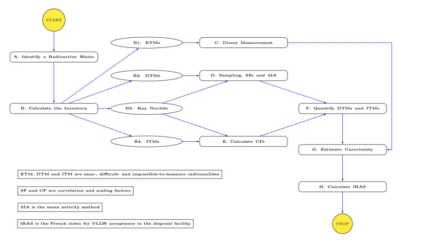
Le schéma global de la méthode de caractérisation est montré en Fig. 2. Les principales étapes du processus sont:
A. Identification d’une population de déchets radioactifs
B. Évaluation de l’inventaire radiologique via calculs analytiques ou simulations Monte Carlo
C. Quantification de l’activité des radionucléides émetteurs γ (ou ETM) par mesure directe
D. Test d’applicabilité des méthodes de ratios d’activité ou activité moyenne pour l’évaluation de l’activité des émetteurs β-purs
E. Quantification des facteurs de corrélation
F. Quantification de l’activité des radionucléides difficiles (DTM) ou impossibles (ITM) à mesurer
G. Estimation de l’incertitude
H. Évaluation de l’acceptabilité du lot de déchets radioactifs au sein du centre d’entreposage final par calcul de l’Indice Radiologique d’Acceptabilité en Stockage (IRAS).
L’Agence National Française pour la Gestion des Déchets Radioactifs (ANDRA) a établi des indices permettant de tester l’acceptabilité d’un colis et d’un lot de colis TFA en
entreposage final. Le premier indice, appelé IRAS, permets de tester l’acceptabilité d’un colis unique de déchets et est défini comme suit:
IRAS =∑
i
ai
10Classei (1)
où ai est l’activité massique du radionucléide i et Classei renseigne sur la radio-toxicité de
ce même radionucléide. Afin qu’un colis de déchets puisse être accepté en entreposage final il est nécessaire que l’IRAS soit inférieur à 10.
Ensuite l’ANDRA a aussi défini un indice fixant des limites d’acceptabilité sur un lot de colis de dechets radioactifs. L’IRAS colis est ainsi défini:
⟨IRAS⟩= ∑ k Mk· IRASk ∑ k Mk (2)
ou Mk est la masse du colis k et IRASk est l’IRAS associé au colis k. Afin qu’un lot de
LONG START
A. Identify a Radioactive Waste
B. Calculate the Inventory B3. Key Nuclide B2. DTMs
B4. ITMs
B1. ETMs C. Direct Measurement
D. Sampling, SFs and MA
E. Calculate CFs
F. Quantify DTMs and ITMs
G. Estimate Uncertainty
H. Calculate IRAS
STOP ETM, DTM and ITM are easy-, difficult- and impossible-to-measure radionuclides
SF and CF are correlation and scaling factors
MA is the mean activity method
IRAS is the French index for VLLW acceptance in the disposal facility
Figure 2: Processus de caractérisation radiologique des déchets métalliques TFA développé au CERN.
2. Évaluation de l’inventaire radiologique
L’inventaire radiologique est la liste des radionucléides produits avec une activité supérieure au seuil de déclaration (SD). Le seuil de déclaration est l’activité massique minimale à partir de laquelle un radionucléide doit être pris en compte lors du calcul de l’IRAS.
La méthodologie décrite dans cette thèse propose l’utilisation de codes de calcul afin d’établir l’inventaire radiologique. Tout particulièrement, afin de prendre en compte un nombre élevé de scenarios d’activation potentiels, un vecteur aléatoire S à cinq composants a été introduit:
S= (CC, E, P, ti, tc). (3)
où:
• CC est un vecteur aléatoire représentant la composition chimique du matériau
• E est l’énergie de l’accélérateur
• P la position du matériau au sein du complexe d’accélérateurs
• ti le temps d’irradiation et
• tcle temps de décroissance.
Lorsque une unique combinaison des composants du vecteur aléatoire S est extraite, nous pouvons l’utiliser comme paramètre d’entrée d’un simulation de type Monte Carlo ou d’un calcul analytique.
Les simulations fournissent d’un coté la liste de tous les radionucléides qui peuvent être produits par activation et de l’autre des facteurs de corrélation permettant d’établir une relation fonctionnelle entre des radionucléides de type ETM (émetteurs γ) et des radionucléides DTM ou ITM.
La différence entre radionucléides DTM et ITM s’opère par le biais de leur contribution à l’IRAS CIRAS
i , défini comme suit:
CiIRAS = ai ALi ∑ j aj ALj . (4)
avec AL étant égal à 10Classe.
Tout particulièrement, si un radionucléide (hors ETM) contribue à l’IRAS plus de 1% alors il est defini difficile-à-mesurer (DTM). Lorsque la contribution d’un radionucléide est inférieure à 1% alors il sera classé comme impossible-à-mesurer (ITM).
La section suivante montre comment évaluer les activités des radionucléides DTM et ITM dans les déchets métalliques TFA produits au CERN.
3. Méthodes pour quantifier l’activité
Chaque radionucléide peut être classifié comme facile à mesurer (ETM), difficile (DTM) ou impossible à mesurer (ITM).
Un radionucléide est défini ETM s’il peut-être mesuré depuis l’extérieur d’un colis de déchets en utilisant des méthodes de mesure non-destructives, comme par exemple la spectrométrie γ.
Un radionucléide est défini DTM si la détermination de son activité massique nécessite des mesures de type destructive (dissolution acide, mesure par scintillation liquide ou comptage α\β).
Un radionucléide est défini ITM si son niveau d’activité massique est systématique-ment inférieur aux seuils de détection des instrusystématique-ments communésystématique-ment employés pour leur mesure. L’activité massique de cette famille de radionucléides est généralement évaluée par simulation numérique.
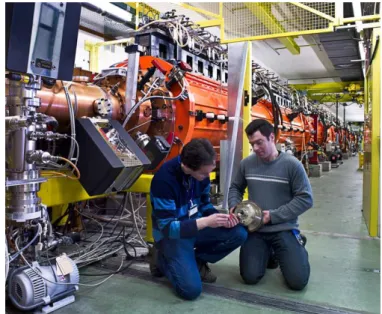
Au CERN, la quantification de l’activité des ETM est faite grâce à des spectrométres γ portatifs, refroidis électriquement. Un exemplaire de ce détecteur est montré en Fig. 3.
Figure 3: Le Falcon5k est un spectrométre γ portable, refroidi électriquement. Ce système de mesure est couramment employé au CERN pour quantifier l’activité des radionucléides ETM dans les colis de déchets radioactifs TFA.
caractérisation) et si son activité massique est corrélée à l’activité des DTM et ITM alors il est défini traceur (KN) et son activité peut etre utilisée pour quantifier l’activité massique des radionucléides DTM et ITM.
Une liste des radionucléides traceurs potentiels pour les déchets métalliques TFA produits au CERN est donnée dans la table qui suit.
Table 1: Liste de traceurs potentiel pour les déchets métalliques TFA. En gras sont identifiés les KN utilisés au CERN à la date d’écriture de cette thèse.
Matériau KNs T1/2 (ans) Émetteur γ principal
Acier
Na-22 2.603 1275 keV
Ti-44 58.9 1157 keV (Sc-44)
Co-60 5.2711 1173 keV, 1332 keV
Cuivre
Na-22 2.603 1275 keV
Ti-44 58.9 1157 keV (Sc-44)
Co-60 5.2711 1173 keV, 1332 keV
Rh-101 3.3 127 keV, 198 keV, 325 keV
Sb-125 2.7586 428 keV, 601 keV, 636 keV
Aluminium
Na-22 2.603 1275 keV
Ti-44 58.9 1157 keV (Sc-44)
Co-60 5.2711 1173 keV, 1332 keV
des ratios d’activité ou de l’activité moyenne. Ces méthodes se basent sur le prélèvement d’échantillons représentatifs à partir de la population de déchets. Chaque échantillon est mesuré par spectrométrie γ et par radiochimie et le ratio d’activité (SF) est calculé:
SFi =
aDT Mi
aKNi
. (5)
où aDT Mi est l’activité massique du DTM dans l’échantillon i et aKNiest l’activité massique
du traceur dans le même échantillon.
Une distribution des SFi peut ensuite être construite. Si les activités des DTM et KN
sont corrélées (en général le coefficient de corrélation doit être supérieur à 0.5) alors il est possible choisir une estimateur de tendance centrale approprié selon la distribution expérimentale obtenue.
La pratique expérimentale montre que, souvent, la moyenne géométrique est un estima-teur robuste pour les ratios d’activité. La moyenne géométrique des ratios d’activité GSF
peut être calculée à l’aide de la formule suivante:
GSF = exp ( 1 n n ∑ i=1 ln(SFi) ) = ( n ∏ i=1 SFi ) 1 n . (6)
Si nous indiquons avec SF le ratio d’activité obtenu à partir des échantillons, alors l’activité massique du DTM i dans le colis j (ˆaDT Mi,j) peut-être calculée par le biais de la
formule suivante:
ˆaDT Mi,j = SF × aKNj (7)
où aKNj est l’activité massique du KN mesurée dans le colis j.
Lorsque la corrélation entre les activités des DTM et KN est inférieure à 0.5, la méthode de la moyenne s’applique. Cette méthode consiste a attribuer à chaque colis l’activité moyenne obtenue à partir de la mesure des échantillons.
Pour conclure, l’activité massique des radionucléides ITM est estimée en applicant un processus similaire de celui décrit pour les radionucléides DTM. La différence réside dans
l’estimation des ratios d’activité que, dans le cas des ITM, est obtenue à partir de codes de calcul.
Si CF indique le ratio d’activité (estimé par calcul) corrélant l’activité des ITM avec le KN, alors l’activité du radionucléide ITM dans le colis j (ˆaIT Mj) est donnée par:
ˆaIT Mj = CF × aKNj. (8)
où aKNj est l’activité massique du KN mesurée dans le colis j.
4. Estimation des incertitudes
Afin d’assurer le respect des critères d’acceptation fournis par l’ANDRA il est essentiel estimer les incertitudes associées à l’IRAS (colis et lot).
Ces incertitudes peuvent être évaluées en utilisant les formules classiques de propagation des incertitudes.
L’incertitude combinée de l’IRAS d’un colis est donnée par:
u2c(IRAS) = n ∑ i=1 u2(ai) AL2 i + n ∑ i=1 i̸=j n ∑ j=1 j̸=i r(ai, aj) · u(ai) · u(aj) ALi· ALj (9)
où u(ai) et u(aj) sont les incertitudes associées aux activités des radionucléides i et j,
r(ai, aj) est la corrélation entre leur activités et ALi et ALj sont les limites d’activité des
radionucléides i et j (AL = 10Classe).
L’incertitude de l’IRAS d’un lot s’obtient par propagation des incertitudes pour des variables non corrélées. Cette hypothèse est valable car l’IRAS d’un colis et le poids sont des quantités non-corrélées. Tout particulièrement, nous obtenons:
u2c(⟨IRAS⟩) ≃ n ∑ k=1 ( M k Mtot )2 · u2(IRAS k) + n ∑ k=1 (IRAS k Mtot )2 · u2(M k) (10)
où Mtot est la masse totale du lot de colis et u2(IRASk) et u2(Mk) sont les incertitudes au
Si l’on divise Eq. 10 par ⟨IRAS⟩2 nous pouvons reformuler l’incertitude comme suit: (u(⟨IRAS⟩) ⟨IRAS⟩ )2 ≃ n ∑ k=1 (u(IRAS k) IRASk )2 + n ∑ k=1 (u(M k) Mk )2 . (11)
Si les incertitudes des IRAS colis sont similaires (u(IRASk) = u(IRAS)) ainsi que les
incertitudes des poids des colis (u(Mk) = u(M)) l’equation de l’incertitude de l’IRAS lot
peut etre simplifiée.
En utilisant la definition de variance nous pouvons écrire:
n ∑ k=1 Mk2= nM2+ nV ar(M) ≃ nM2+ ns2(M) (12) et n ∑ k=1
IRASk2= nIRAS2+ nV ar(IRAS) ≃ nIRAS2+ ns2(IRAS) (13) où s2 represente le carré de l’écart-type expérimentale de M et IRAS, et M et IRAS sont les poids et IRAS moyens.
Si nous injectons les deux dernières équations dans la formule générale de l’incertitude de l’IRAS d’un lot de déchets nous pouvons calculer:
u2c(⟨IRAS⟩) ≃ 1 Mtot2 [ u2(IRAS)(nM2+ ns2(M))]+ 1 M2 tot [ u2(M)(nIRAS2+ ns2(IRAS))]. (14) En fin, si on écrit M2 tot = nM 2
nous obtenons la formule définitive pour calculer l’incertitude associée à l’IRAS d’un lot de déchets radioactifs:
u2c(⟨IRAS⟩) ≃ u 2(IRAS) n ( 1 +s2(M) M2 ) + u2(M) M2 ( IRAS2 n + s2(IRAS) n ) . (15)
5. Résultats
La méthode de caractérisation proposée dans cette thèse a été testée et validée dans le cadre du projet SHERPA, le plus grand projet d’élimination de déchets radioactifs TFA réalisé au CERN entre 2014 et 2017.
L’objectif du projet SHERPA est celui de créer un processus de caractérisation, traite-ment et élimination de plus de 1000m3 de déchets radioactifs métalliques TFA. Le sommaire du nombre de colis caractérisés dans le cadre du projet SHERPA est présenté en Tab. 2. Table 2: Sommaire des colis traités dans le cadre du projet SHERPA jusqu’à juin 2017. 80% de ces colis sont en entreposage définitif. La partie restante est caractérisée et prête pour l’expédition.
Matériau N. colis Poids (en tonnes)
Aluminium 68 81.6
Cuivre 17 38.7
Acier 262 572.4
Total 347 692.7
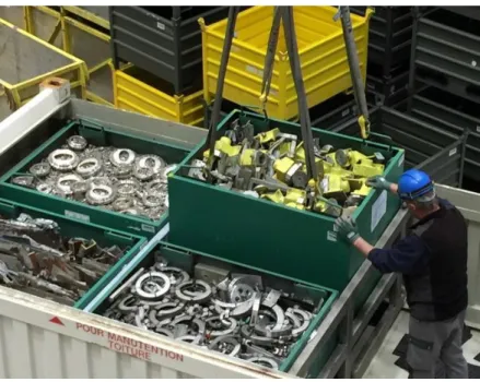
Un exemple de colis en cours de préparation pour l’expédition est donné en Fig. 4.
Figure 4: Chargement d’un lot de colis de déchets SHERPA pour expédition en entreposage.
un nombre élevé de scénarios d’activation (>2.35 millions), pour tous les matériaux couramment utilisés au CERN, toutes les énergies des accélérateurs et pour des temps d’irradiation et de décroissance allant de 1 jusqu’à 40 ans.
L’inventaire radiologique obtenu pour les familles de métaux plus courants est donné en Tab. 3.
Table 3: Inventaire radiologique pour les familles de métaux traités dans le cadre du projet SHERPA. Environ 2.35 millions de scénarios d’activation ont été pris en compte.
Famille ETM DTM/ITM
Aluminium Na-22, Al-26, Ti-44, Mn-54 H-3, C-14, Cl-36, Ar-39
Co-57, Co-60, Zn-65 Fe-55, Ni-63
Cuivre
Na-22, Ti-44, Mn-54, Co-57
Co-60, Zn-65, Mo-93, Rh-101 H-3, C-14, Cl-36, Ar-39
Ag-108m, Ag-110m, Sn-121m, Sb-125 Ca-41, Fe-55, Ni-63
Gd-148, Hg-194, Bi-207 Acier
Na-22, Ti-44, Mn-54, Co-57 H-3, Be-10, C-14, Cl-36
Co-60, Zn-65, Mo-93, Nb-93m Ar-39, Ca-41, Fe-55
Nb-94, Tc-99 Ni-63
De tous les radionucléides prévus par calcul, seulement une partie dépasse les seuils de déclaration et doit donc être utilisée pour le calcul de l’IRAS. Les ETM dépassant les seuils de déclaration sont indiqués dans en Tab. 4. Les distributions d’activité massique pour Co-60 et Na-22 sont montrées en Fig. 5.
Table 4: Liste des radionucléides ETM dépassant les seuils de déclaration dans le cadre du projet SHERPA.
Matériau ETM
Aluminium Na-22, Ti-44, Co-60, Ag-108m
Cuivre Ti-44, Co-60, Ag-108m
Acier Ti-44, Mn-54, Co-60, Zn-65, Ag-108m, Bi-207
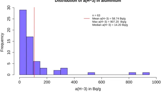
Les radionucléides DTM dépassant les seuils de déclaration sont H-3, Fe-55 et Ni-63. La distribution des activités massiques du H-3 dans l’aluminium est montrée comme un exemple en Fig. 6.
Pour conclure, les ITM détectés au delà du seuil de déclaration sont C-14 (19 colis), Cl-36 (19 colis) et Ar-39 (15 colis). Cependant, leur impact sur l’IRAS est négligeable.
Distribution of a(Co−60) in steel a(Co−60) in Bq/g Frequency 0 2 4 6 8 10 12 14 0 10 20 30 40 50 60 70 n = 154 Mean a(Co−60) = 0.94 Bq/g Max a(Co−60) = 13.83 Bq/g Median a(Co−60) = 0.55 Bq/g
Distribution of a(Na−22) in aluminium
a(Na−22) in Bq/g Frequency 0 1 2 3 4 0 2 4 6 8 10 12 n = 27 Mean a(Na−22) = 0.70 Bq/g Max a(Na−22) =3.59 Bq/g Median a(Na−22) = 0.21 Bq/g
Figure 5: Histogrammes des activités massiques pour Co-60 et Na-22 en acier et aluminium. La figure montre seulement les activités qui dépassent les seuils de déclaration. Les lignes rouges indiquent les activités moyennes.
Distribution of a(H−3) in aluminium
a(H−3) in Bq/g Frequency 0 200 400 600 800 1000 0 5 10 15 20 25 30 n = 63 Mean a(H−3) = 58.74 Bq/g Max a(H−3) = 907.20 Bq/g Median a(H−3) = 14.20 Bq/g
Figure 6: Histogramme de l’activité spécifique du H-3 dans des déchets d’aluminium. Seulement les valeurs dépassant les seuils de déclaration sont montrées. La ligne rouge indique l’activité massique moyenne du H-3.
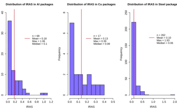
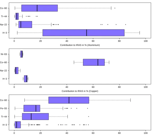
radionucléides en présence, il est possible d’évaluer l’IRAS des colis et l’IRAS lot. Les graphiques qui suivent présentent les sommaires des IRAS colis pour le projet SHERPA
et par famille de matériau. La contribution de chaque radionucléide à l’IRAS est aussi donnée.
Distribution of IRAS in Al packages
IRAS Frequency 0.0 0.2 0.4 0.6 0.8 1.0 1.2 0 10 20 30 40 n = 68 Mean = 0.18 Max = 1.06 Median = 0.1
Distribution of IRAS in Cu packages
IRAS Frequency 0.0 0.1 0.2 0.3 0.4 0.5 0 2 4 6 8 n = 17 Mean = 0.13 Max = 0.39 Median = 0.08
Distribution of IRAS in Steel packages
IRAS Frequency 0.0 0.5 1.0 1.5 2.0 0 50 100 150 200 250 n = 262 Mean = 0.10 Max = 1.93 Median = 0.06
Figure 7: Histogrammes des IRAS colis pour les trois familles de metaux du projet SHERPA. Les lignes rouges indiquent les valeurs moyenne de l’IRAS colis.
6. Conclusions
L’objectif de ce travail de thèse est celui de proposer une solution pour la caractérisation radiologique des déchets métalliques TFA produits au sein des accélérateurs de particules. La méthode proposée se base sur une combinaison de simulations numériques et mesures permettant d’établir l’inventaire radiologique, d’évaluer l’activité des radionucléides plus importants et d’évaluer l’acceptabilité des colis de déchets dans les centres d’entreposage à partir du calcul de l’indice IRAS.
Le processus de caractérisation ici décrit est aujourd’hui employé en routine pour la caractérisation des déchets radioactifs métalliques produits au CERN. Cette méthode est acceptée par l’ANDRA, est applicable à la majorité de déchets métalliques et peut être facilement adaptée à d’autre familles de déchets.
H−3 Na−22 Ti−44 Co−60
0 20 40 60 80 100
Contribution to IRAS in % (Aluminium)
H−3 Na−22 Co−60 Ni−63
0 20 40 60 80 100
Contribution to IRAS in % (Copper)
H−3 Ti−44 Fe−55 Co−60
0 20 40 60 80 100
Contribution to IRAS in % (Steel)
Figure 8: Contribution des radionucléides principaux à l’IRAS pour les 347 colis de déchets radioactifs du projet SHERPA traités avant juin 2017.
Le travail de cette thèse a aussi permis d’augmenter la taille des déchets caractérisés et éliminés au CERN: nous sommes passés de la caractérisation de peu d’objets avec une histoire radiologique connues à des centaines de tonnes de déchets avec histoire radiologique peu ou pas connue.
Nous avons aussi démontré que l’impact des éléments trace dans les matériaux est négligeable en termes d’inventaire radiologique.
La partie centrale du travail de thèse regarde l’adaptation de la méthode des ratios d’activité aux besoins du CERN. Cette méthode a en effet été adaptée et validée et est aujourd’hui à la base de la quantification de l’activité des radionucléides DTM.
Un point de force de la nouvelle méthode de caractérisation réside dans sa capacité de concentrer l’effort de caractérisation sur les radionucléides qui contribuent le plus à l’IRAS. Pour ce faire, des critères statistiques ont été développés et utilisés. Cela a en effet permis d’appliquer les méthodes de caractérisation plus longues et couteuse seulement aux radionucléides qui ont un impact avéré sur l’IRAS.
Pour conclure, la méthode de caractérisation proposée dans cette thèse est aujourd’hui implémentée à une échelle industrielle au CERN. La méthode a permis la caractérisation ou élimination d’environ 690 tonnes de déchets métalliques TFA entre 2015 et 2017 et peut être facilement adaptée à la caractérisation de nouvelles familles de déchets radioactifs.
I would like to express my personal thanks to my CERN supervisor Dr. Matteo Magistris because his guidance has been warm and illuminating. He is an invaluable mentor, kind and has always kept a sense of humour when I had lost mine. Today, thanks to his continuous example, I am a better person.
My thanks go also to Dr. Luisa Ulrici, the head of CERN radioactive waste section. This work would have not seen the light of day without her support and sponsorship.
I am infinitely grateful to my professors Catherine Luccioni, Jean-Pierre Chevalier and Gilbert Saporta. Their advice has always been precise, concrete and, most of all, useful.
Pr. Luccioni has followed closely my career since the very beginning, when I was a young γ-spectrometry technician. Today, after many years, her wise presence is still comforting and encouraging. In addition, her attention to details drove me to learn to finally punctuate my prose better.
Pr. Jean-Pierre Chevalier has expertly guided me through my PhD journey. His advice to “focus on what is really important” is discreetly pinned over my desk and has been a guidance for my work and my life until this day.
I am grateful, beyond words, to Pr. Gilbert Saporta for helping me to discover the beautiful world of statistics and data analysis. If today I am pondering about a career in statistics it is surely because of his example.
I would like to express my deepest gratitude to Pr. Abdallah Lyoussi, Dr. Bertrand Iooss and Mr. Michel Dutzer for accepting to be part of the committee of my PhD thesis. Their comments were very precious and have allowed me to look at my work from a different perspective.
I would like to finish by thanking my family, friends and colleagues. They created the perfect environment for me to reach this goal.
First of all my wife Julia, for her constant support and for reminding me that work is only one aspect of life and that I am surrounded by a lot of beautiful things to look at.
Stealing the words of a far better person than myself, I would like to thank my parents for the greatest gift: poverty. If that is the baseline, everything else is an enjoyable conquest to watch with the eyes of wonder.
A special thanks goes to my colleagues and friends Elpida, Francesco and Sven. They made my lunches less lonely, my weekends funnier and my life richer by far.
To conclude, thanks to Asimov, Bufalino, Dostoevsky, Eco, Gary, Kristof, Marquez, Murakami, Pamuk, Rand, Rushdie, Saramago, Singer and the many many others whose literature has allowed me to enjoy countless, sleepless nights and to visit beautiful, unknown worlds.
Abstract 3
Résumé 5
Résumé long en langue française 7
Acknowledgements 23 Contents 25 List of Tables 28 List of Figures 32 Acronyms 39 Introduction 41 1 General context 45
1.1 CERN’s accelerator complex . . . 46 1.2 Beam losses, particle spectra and induced radioactivity . . . 53 1.2.1 Beam dynamics . . . 53 1.2.2 Hypothesis on beam losses . . . 55 1.2.3 Particle spectra . . . 57
1.2.4 Induced radioactivity . . . 59 1.3 Radioactive waste and disposal pathways . . . 61 1.3.1 VLLW disposal pathway . . . 61 1.3.2 Clearance . . . 62 1.3.3 Radioactive waste from CERN accelerators . . . 64 1.4 Radiological characterization . . . 66 1.4.1 New and legacy waste . . . 67 1.4.2 The radiological characterization workflow . . . 68
2 Evaluation of the radionuclide inventory 73
2.1 Calculation and simulation codes . . . 78 2.1.1 Monte Carlo methods and the Fluka code . . . 78 2.1.2 The Fluka input file . . . 80 2.1.3 Actiwiz . . . 82 2.2 Elemental composition . . . 85 2.3 Position within the tunnel and beam energy . . . 96 2.4 Irradiation and decay times . . . 100 2.5 Selecting the number of realisations . . . 102 2.6 Radionuclide inventory of cathodic copper . . . 105
3 Methods to quantify the activity 111
3.1 Activity quantification of ETM radionuclides . . . 113 3.1.1 γ-ray spectrometry . . . 113 3.1.2 Practical aspects in gamma-spectrometry . . . 119 3.1.3 Selection of potential key nuclides for metallic waste . . . 122 3.2 Activity quantification of DTM radionuclides . . . 124 3.2.1 The scaling factor method . . . 124
3.2.2 Mean activity method and bootstrap . . . 129 3.2.3 Probability and authoritative sampling . . . 132 3.2.4 Radiochemical analysis . . . 143 3.3 Activity quantification of ITM radionuclides . . . 147 3.3.1 Multiple linear regression . . . 151 3.3.2 Decision trees . . . 161
4 Uncertainty quantification 165
4.1 The GUM framework . . . 166 4.2 Quantification of ETM’s uncertainty . . . 172 4.2.1 Analytical uncertainty . . . 173 4.2.2 Bias . . . 174 4.3 Quantification of DTM’s uncertainty . . . 177 4.3.1 Analytical uncertainty of scaling factors . . . 177 4.3.2 Analytical uncertainty of the mean activity . . . 178 4.3.3 Bias . . . 179 4.4 Quantification of ITM’s uncertainty . . . 180 4.5 Propagating uncertainties . . . 183
5 Case study, results and discussion 189
5.1 Radiological characterization of copper from shredded cables . . . 190 5.1.1 The waste population . . . 190 5.1.2 Calculation of the radionuclide inventory . . . 194 5.1.3 Quantification of ETM’s activity . . . 195 5.1.4 Quantification of DTM’s activity . . . 198 5.1.5 Quantification of ITM’s activity . . . 201 5.1.6 Calculation of IRAS . . . 203
5.2 The SHERPA project . . . 205 5.2.1 The waste population . . . 205 5.2.2 Calculation of the radionuclide inventory . . . 209 5.2.3 Quantification of ETM’s activity . . . 213 5.2.4 Quantification of the activity of DTMs and ITMs . . . 216 5.2.5 Calculation of IRAS . . . 222 5.3 Discussion . . . 224 5.3.1 Time and financial aspects of the characterization . . . 224 5.3.2 Limits, ongoing improvements and future work . . . 227
Conclusion 237
1 Liste de traceurs potentiel pour les déchets métalliques TFA. En gras sont identifiés les KN utilisés au CERN à la date d’écriture de cette thèse. . . . 13 2 Sommaire des colis traités dans le cadre du projet SHERPA jusqu’à juin
2017. 80% de ces colis sont en entreposage définitif. La partie restante est caractérisée et prête pour l’expédition. . . 17 3 Inventaire radiologique pour les familles de métaux traités dans le cadre du
projet SHERPA. Environ 2.35 millions de scénarios d’activation ont été pris en compte. . . 18 4 Liste des radionucléides ETM dépassant les seuils de déclaration dans le
cadre du projet SHERPA. . . 18
1.1 Main parameters of the LHC. . . 52 1.2 Estimated particle losses per machine for the design power loss of 1 W/m. . 57 1.3 Half-life (T1/2), VLLW class and Declaration Threshold (DT) of common
radionuclides of activated metals in hadron accelerators [ANDRA 2013a]. Columns 4 and 5 give reference values for clearance in Switzerland [ord 1994]. LE is the so-called Exemption Limit and CS is the Surface Contamination. 63
2.1 Radionuclide inventory generated by irradiation of copper CuOFE [Froeschl et al. 2012] behind concrete shielding of the LHC. The irradiation lasted for 7 days followed by 2 years of decay. . . 84
2.2 IRAS top contributors obtained by activating copper CuOFE behind concrete shielding of the LHC. The irradiation lasted for 7 days followed by 2 years of decay. . . 85 2.3 Philosophy for setting basic type of distributions of chemical elements.
Adapted from [ISO 2013]. . . 87 2.4 Elemental composition of world-wide copper concentrates [CDA 2004]. The
values of the quantiles for a given percentile p are in %. The number of samples considered for the analysis is n = 119. . . 91 2.5 Distribution parameters (µ, σ) obtained from quantiles for impurities in
world-wide copper concentrates. . . 93 2.6 Comparison between median and mode of the distributions of trace elements
obtained from copper concentrates [CDA 2004] and maximum allowed impurities in electrolytic cathodic copper (Grade A) as specified by the standards ASTM B115 [ASTM 2016] (Grade 1 and 2) and [BS 1998] (Cu-CATH-1). The values are in ppm. . . 93 2.7 Radionuclide inventory of cathodic copper obtained extracting 10000
ran-dom realizations from the ranran-dom vector scenario. Only radionuclides contributing at least 0.05% to the IRAS are showed. . . 106
3.1 List of potential key nuclides for metallic VLLW characterization. In bold are given the key nuclides presently used for these material families. . . 123 3.2 Case study of pure iron irradiated for 1 year at the LHC. The material,
which was located close to the tunnel wall, is left to decay for 10 years. The contribution to the IRAS is calculated together with the activities for IRAS = 10. The specific activity aiis obtained from analytical calculations performed
with Actiwiz [Theis and Vincke 2012] and is given in Bq/g/primary/second.150 3.3 Output of the linear model obtained from 10000 realizations of activated
cathodic copper. The pair Ni-63/Co-60 is considered for the calculations of the CF. . . 154
5.1 Average density and average amount of metal of the 5 families of VLLW cables identified at CERN. The uncertainty is calculated as the standard error of the mean (k=1) [La Torre and Magistris 2016]. . . 191 5.2 Summary statistics of the preliminary γ-screening performed on the copper
waste population. The reference date for the Co-60 equivalent specific activity is 01/07/2015. . . 194 5.3 Summary statistics of the measurements performed on 87 composite samples
of shredded copper. The reference date for the specific activity is 01/07/2015. Last line indicates the Declaration Thresholds of the various nuclides. . . . 197 5.4 Summary statistics of the relative standard deviation urel (in %, k=1)
associated with the activities of the major radionuclides in the copper waste population. . . 204 5.5 Summary of the SHERPA disposal campaigns as of June 2017. Above 80%
of the packages is already stored at the ANDRA disposal facilities. The remaining waste packages are characterized and ready to be shipped. About 20% of the waste originate from electron machines. . . 208 5.6 Summary data of the major material grades considered for the calculation
of the radionuclide inventory for the SHERPA project. . . 210 5.7 Predicted radionuclide inventories of VLLW metals activated at CERN.
Above 2.35 million irradiation scenarios were considered. . . 210 5.8 Predicted radionuclide inventories of VLLW pipes made of stainless steel
and activated at the LEP accelerator. . . 212 5.9 List of ETM radionuclides quantified above the Declaration Threshold per
material type. The table includes radionuclides produced at both proton and electron accelerators. . . 213 5.10 List of DTM radionuclides quantified above the Declaration Threshold per
5.11 Summary of mean activities and scaling factors for the campaigns of the SHERPA project characterized between 2015 and 2017. . . 218 5.12 Summary of correlation factors for aluminium and copper waste characterized
between 2015 and 2017. . . 221 5.13 Summary of correlation factors for steel waste characterized between 2015
and 2017. . . 221 5.14 Comparison of major radionuclides obtained with cathodic copper and copper
CuOFE. CIRAS is the contribution of a given radionuclide to the IRAS. . . 229
5.15 Comparison of correlation factors and scaling factors for the disposal waste campaigns 2 to 4. The lower and upper boundaries in parentheses are given within a 95% confidence level. . . 230
1 Complexe d’accélérateurs de particules du CERN. . . 7 2 Processus de caractérisation radiologique des déchets métalliques TFA
développé au CERN. . . 10 3 Le Falcon5k est un spectrométre γ portable, refroidi électriquement. Ce
système de mesure est couramment employé au CERN pour quantifier l’activité des radionucléides ETM dans les colis de déchets radioactifs TFA. 13 4 Chargement d’un lot de colis de déchets SHERPA pour expédition en
entreposage. . . 17 5 Histogrammes des activités massiques pour Co-60 et Na-22 en acier et
aluminium. La figure montre seulement les activités qui dépassent les seuils de déclaration. Les lignes rouges indiquent les activités moyennes. . . 19 6 Histogramme de l’activité spécifique du H-3 dans des déchets d’aluminium.
Seulement les valeurs dépassant les seuils de déclaration sont montrées. La ligne rouge indique l’activité massique moyenne du H-3. . . 19 7 Histogrammes des IRAS colis pour les trois familles de metaux du projet
SHERPA. Les lignes rouges indiquent les valeurs moyenne de l’IRAS colis. . 20 8 Contribution des radionucléides principaux à l’IRAS pour les 347 colis de
déchets radioactifs du projet SHERPA traités avant juin 2017. . . 21
1.1 Schematic layout of the CERN’s accelerator complex. . . 47 1.2 Linac 2, at the beginning of the CERN’s accelerator chain. . . 48 1.3 A section of the PS Booster. . . 49
1.4 A section of the PS during maintenance. . . 49 1.5 View of the SPS tunnel. . . 50 1.6 A section of the LHC, the world’s largest particle accelerator. . . 51 1.7 Example of horizontal phase space for a generic section of the LHC. Here
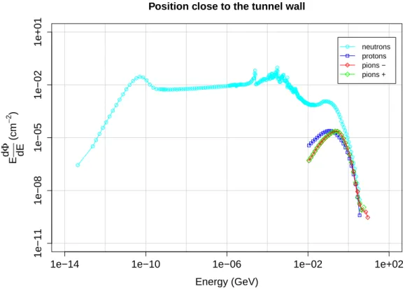
γ(s) = [1 + α2(s)]/β(s). Adapted from [Bruce et al. 2014] and [Wilson 2001]). . . 56 1.8 Particle fluence generated by a current of one proton per second inside the
LHC, when the position is close to the concrete tunnel wall (the data used to build the spectrum is a courtesy of H. Vincke and C. Theis, CERN). . . 58 1.9 Particle fluence generated by a current of one proton per second inside the
LHC for the beam impact area (the data used to build the spectrum is a courtesy of H. Vincke and C. Theis, CERN). . . 59 1.10 Radiological characterization process developed at CERN for VLLW metallic
waste. . . 70
2.1 First stages of the radiological characterization process. ETMs, DTMs and ITMs stand for easy-, difficult- and impossible-to-measure radionuclides. . . 74 2.2 An example of waste family produced and stored at CERN. These metallic
elements are accelerating cavities of the LEP machine. . . 75 2.3 An example of activated cables produced at CERN, presently being disposed
of as VLLW. . . 75 2.4 Experimental normal distribution of cathodic and unalloyed copper from
measurements on incremental random samples performed on radioactive cables. . . 90 2.5 Calculated distributions of impurities from concentrates of copper [CDA
2004]. The probability densities are built from 119 representative samples. . 94 2.6 Standard locations implemented in Actiwiz (version 2) [Theis and Vincke
2.7 Histograms of waste items recorded as a function of the decay time estimated from the date of reception at the CERN’s storage centre. . . 101
2.8 Selection of the number of scenarios using the stabilization of the parameters of the log-normal distribution. In blue (top) are given the geometric mean CFs for Ni-63 and H-3 in cathodic copper. In red (bottom) are presented the variations of the geometric standard deviations for the same radionuclides with the number of scenarios. . . 105
3.1 Stages of the radiological characterization process to determine the activity of the radionuclides in VLLW. ETMs, DTMs and ITMs stand for easy-, difficult- and impossible-to-measure radionuclides. SF, CF and MA stand for scaling factor, correlation factor and mean activity method. . . 112
3.2 Falcon5k is an electrically chilled and portable γ-ray detector. This system is commonly used at CERN to quantify the activity of ETM radionuclides in radioactive waste. . . 114
3.3 Example of calibrations for a standard 1.3 m3 container filled with pure iron radioactive waste and measured with the Falcon5k. The top plot represents the efficiency calibration function. The bottom-left plot shows the resolution (in red) and the low-tail deformation (in blue). The bottom-right graph
represents the energy calibration curve. . . 117
3.4 A batch of 1.3 m3 packages containing metallic VLLW. Credits: B. Cellerier, CERN. . . 121
3.5 Log-normal distributions of Ni-63 and Co-60 specific activities and log-normal distribution of their ratio obtained by simulating the irradiation of cathodic copper at 10000 random CERN scenarios. The average content statistics geometric mean (gray), mean (red) and median (green) are represented together with the normal curve. The x-axis is in log-scale. . . 126
3.6 Left: a histogram of the estimates of a(Ni-63) obtained by generating 1000 simulated datasets from the true population. Center: a histogram of the estimates of a(Ni-63) obtained from 1000 bootstrap samples from a single dataset. Right: the estimates of a(Ni-63) displayed in the left and center panels are shown as boxplots. In each panel, the gray line indicates the true value of a(Ni-63). This plot is adapted from [James et al. 2017]. . . 132 3.7 Scatter plot matrix of a selected number of variables when 10000 realizations
of the multivariate random vector are selected. The CF is calculated for the pairs Ni-63/Co-60 . . . 153 3.8 Parameter selection using backward stepwise selection coupled with R2
statistic. . . 155 3.9 Example of evolution of CFs and activity with time. The pairs Ni-63/Co-60
(left plot), Fe-55/Ti-44 (central plot) and Fe-55/Na-22 (right plot) are treated.157 3.10 Evolution of the CF Ni-63 vs Co-60 with time from 10000 random scenarios. 158 3.11 Diagnostic plots for the study of the regression model. . . 159 3.12 Evolution of correlation factors with the energy and the position within the
accelerators. The case of Ni-63/Co-60 is showed. . . 160 3.13 Regression tree of the correlation factor Ni-63/Co-60. . . 162
4.1 Last stages of the radiological characterization process developed at CERN for metallic VLLW. DTMs and ITMs stand for difficult- and impossible-to-measure radionuclides. SF, CF and MA stand for scaling factor, correlation factor and mean activity method. . . 166 4.2 Monte Carlo scheme used to estimate the uncertainty of a measurand Y
based on the distribution of three input variables via a functional relationship f. Adapted from [JCGM 2008b] [METAS 2012]. . . 171
5.1 Sample CR-049963 of aluminium power cable (φ = 1.8cm). Photo credit: F.P. La Torre, CERN. . . 192
5.2 Sample CR-049985 of copper signal cable (φ = 2cm). Photo credit: F.P. La Torre, CERN. . . 192 5.3 Sample CR-049721 of copper/aluminium coaxial cable (φ = 6.5cm). Photo
credit: F.P. La Torre, CERN. . . 192 5.4 Example of shredded copper. . . 193 5.5 Collected samples of copper shreds. . . 196 5.6 Specific activity distribution of Co-60 in the waste population made of 87
drums of shredded copper from cables. The error bars are given for a coverage factor k=1. For the 6 packages with specific activity below the MDA, the specific activity is replaced by the MDA and the uncertainty is calculated as MDA/2. The green line indicates the average Co-60 specific activity for the entire population. In red it is showed the Declaration Threshold of Co-60 (0.1 Bq/g). . . 198 5.7 Study of the linear model of H-3 vs Co-60. The first plot shows the scatterplot
of the activities together with the regression lines with ˆβ0 = 0 (gray) and ˆβ0 ̸= 0 (red). The plots 2-to-4 present the dispersion, the histogram and the normal qq-plot of the residuals. . . 200 5.8 Study of the linear model of Ni-63 vs Co-60. The first plot shows the
scatterplot of the activities together with the regression lines with ˆβ0= 0 (gray) and ˆβ0 ̸= 0 (red). The plots 2-to-4 present the dispersion, the
histogram and the normal qq-plot of the residuals. . . 200 5.9 Activity distribution of H-3 in the waste population made of 87 drums of
shredded copper from cables. The error bars are given for a coverage factor k=1. In green is showed the average activity (0.38 Bq/g) and in red the Declaration Threshold (1 Bq/g). . . 201 5.10 Activity distribution of Ni-63 in the waste population made of 87 drums of
shredded copper from cables. The error bars are given for a coverage factor k=1. In green is showed the average activity (0.65 Bq/g) and in red the Declaration Threshold (10 Bq/g). . . 202
5.11 The top plot shows the IRAS and its standard deviation (k=1) for the 87 waste packages of very-low-level radioactive copper activated at CERN. The bottom plot illustrates the distributions of the contribution of the uncertainty of each radionuclide’s activity to the total IRAS uncertainty. Radionuclides whose activity’s uncertainty contributes less than 0.1% are omitted for clarity.203 5.12 Processing of a radioactive waste item by the press-shears [Bruno et al. 2017].207 5.13 Example of massive objects disposed of as VLLW waste in 2016. . . 208 5.14 Loading of standard packages filled with metallic VLLW ready for transport
to the ANDRA disposal facility [Bruno et al. 2017]. . . 209 5.15 Spectrometric measurement system deployed at CERN for the measurement
of ETM radionuclides [Bruno et al. 2017]. . . 214 5.16 Histograms of the specific activities of Co-60 in steel and Na-22 in aluminium.
The figure shows only the values above the Declaration Threshold. The red line indicates the average specific activity. Waste produced at both hadron and electron machines are included. . . 215 5.17 Histogram of the specific activity of H-3 in aluminium from both hadron and
electron accelerators. The figure shows only the values above the Declaration Threshold. The red line indicates the average specific activity. . . 217 5.18 Histograms of the IRAS calculated for the three material families of the
SHERPA project. The red line indicates the average IRAS. . . 222 5.19 Contribution of major radionuclides to the IRAS for the 347 waste packages
AA Antiproton Accumulator AC Antiproton Collector AD Antiproton Decelerator
ALICE A Large Ion Collider Experiment
ANDRA French National Agency for Radioactive Waste Management ATLAS A Toroidal LHC ApparatuS
CERN European Organization for Nuclear Research CF Correlation factor
CMS Compact Muon Solenoid
CNGS CERN Neutrinos to Gran Sasso
COMPASS COmmon Muon and Proton Apparatus for Structure and Spectroscopy CS Surface Contamination
DT Declaration Threshold DTM Difficult-to-measure ETM Easy-to-measure
FOPH Federal Office of Public Health
GUM Guide to the expression of uncertainty in measurement IAEA International Atomic Energy Agency
IRAS Indice Radiologique d’Acceptabilité en Stockage ISOLDE Isotope mass Separator On-Line facility
ISR Intersecting Storage Ring ITM Impossible-to-measure
JCGM Joint Committee for Guides in Metrology
KN Key nuclide
LE Exemption Limit
LEAR Low Energy Antiproton Ring LEIR Low Energy Ion Ring
LEP Large Electron-Positron collider LSC Liquid scintillation counting LHC Large Hadron Collider
LHCb Large Hadron Collider beauty MA Mean activity method
MCA Multi-channel analyser
MDA Minimum Detectable Activity nTOF neutron Time-of-Flight
ORaP Ordonnance sur la Radioprotection PS Proton Synchrotron
SC Synchro-Cyclotron
SF Scaling factor
SPS Super Proton Synchrotron TFA Trés Faible Activité VLLW Very-low-level waste
If knowledge can create problems, it is not through ignorance that we can solve them.
Isaac Asimov
Asimov’s guide to science.
Radioactive waste is produced at particle accelerators as a consequence of the interaction of particle beams with matter. The principal mechanism of waste production in these facilities is the activation of the materials surrounding the particle beams. Neutrons, protons, pions and photons can interact with matter and produce unstable nuclei which will lose their energy in excess via radioactive decay.
Activated materials that cannot be reused or recycled need to be disposed of in dedicated disposal facilities. One of the steps needed to dispose of radioactive waste is the so-called radiological characterization. The radiological characterization of a waste consists of establishing the list of produced radionuclides and evaluating their activity.
In the present thesis we introduce a new characterization strategy, based on numerical experiments and measurements, that allows us to safely dispose of legacy very-low-level waste (VLLW) produced at CERN. According to the definition of the International Atomic Energy Agency (IAEA), VLLW is “waste that does not need a high level of containment and isolation and, therefore, is suitable for disposal in near surface landfill type facilities with limited regulatory control” [IAEA 2009a]. VLLW represents the vast majority of the total amount of radioactive waste currently stored at CERN and that will be produced in the future. A specific methodology to characterize this family of waste was therefore needed.
performed to estimate reference radiological inventories for common materials used at particle accelerators such as copper, steel and aluminium. We use destructive and non-destructive nuclear measurements to quantify the activities of the radionuclides and to test for their correlation. Some radionuclides are easily measurable using non-destructive assay methods and we will refer to them as ETM radionuclides. In the context of this work ETM radionuclides are the ones measurable via γ-ray spectrometry. Common examples of ETMs encountered on radioactive metallic waste are Co-60, Na-22 and Ti-44. Radionuclides that require complex destructive methods for the quantification of their activity are called difficult-to-measure (DTM). This second category mainly includes pure β-emitters, such as Ni-63, and low-energy X-ray emitters, such as Fe-55.
Various techniques were developed for the radiological characterization of waste produced in nuclear power plants. One can cite the known scaling factor (SF) and correlation factor (CF) methods. These methods are standardized and useful information can be found in a number of references such as [IAEA 2007] [ISO 2007] [ISO 2013] [IAEA 2009b]. We adapted and implemented some of these methods to take into account the peculiarities of radioactive waste from particle accelerators.
The main result of the present work is the design and implementation of a procedure to radiologically characterize very-low-level waste produced at CERN. The methodology is accepted by the French National Agency for Radioactive Waste Management (ANDRA) and has allowed the characterization of more than 690 tons of activated metals between 2015-2017.
This thesis consists of 6 chapters. Chapter 1 describes the context of the present study. It introduces the CERN’s accelerator complex and the beam losses at the origin of the activation mechanisms. After the introduction of the terminology used in the thesis, the chapter discusses the technical requirements that a waste must respect to be accepted into a final disposal facility. A list of the major waste populations that are presently stored at CERN is then given. The chapter ends with a general overview of the radiological characterization process we developed.
Chapter 2 deals with the calculations performed to estimate the radionuclide inventory of activated materials. After that the perimeter of a waste population is defined, information
about its origin, its chemical composition, its volume and its radiological history is collected. This data is crucial to estimate preliminary radiological inventories. For legacy waste such a set of information is often missing and, only in the best cases, partial or incomplete. In this chapter we introduce a numerical method that allows us to make predictions even if the input data is limited or missing.
Chapter 3 describes the instrumental and analytical techniques used to quantify the activity of the radionuclides in a waste population. We introduce γ-ray spectrometry for the measurement of ETM radionuclides and the scaling factor (SF) and the mean activity (MA) methods to estimate the activity of DTM radionuclides. Some difficult-to-measure radionuclides have such a low activity that often cannot be measured within a reasonable time/cost framework. Moreover, their activity is often below the detection capability of the common instruments used for their quantification. The IAEA decided to name this category of radionuclides impossible-to-measure (ITM) [IAEA 2007].
From a practical point of view ITM radionuclides are similar to DTMs because they cannot be measured from outside a waste package using non-destructive assay techniques. ITMs however differ from DTMs because their activity can only be estimated via analytical calculations. In Ch. 3 we also discuss the difference between DTMs and ITMs, we introduce some techniques to sample radioactive waste and we shortly describe how statistical learning approaches can be used to estimate theoretical correlation factors between ETM and DTM radionuclides.
Chapter 4 deals with the quantification of uncertainty in the characterization process. We list the major terms that contribute to the uncertainty budget following the recom-mendations of the Guide to the expression of uncertainty in measurement (GUM) [JCGM 2008a]. For some terms of the uncertainty budget we cannot apply the classical techniques used to quantify uncertainties. For these cases we implemented a Monte Carlo method and applied statistical learning techniques that can be used in support of the uncertainty evaluation.
Chapter 5 is divided into three major sections. The first part describes the application of the radiological characterization procedure to a population of activated copper. The waste consists of ∼8.5 tons of copper recovered after shredding historical cables extracted
from the accelerators tunnels. We show how to establish the radionuclide inventory, how to calculate scaling and correlation factors and how the specific activity of each radionuclide is estimated using both measurements and calculations. We finally present the calculation of the parameters needed to evaluate the acceptability of the waste in the disposal facility.
The second section of the chapter describes the operational results obtained applying the new characterization method at CERN, with a focus on the metallic waste disposed of in 2015-2017. We present a feedback and the lessons learned from the disposal campaigns completed during this period.
We end the chapter with an overview of key operational parameters which are of interests for the characterization of waste. We finally list and discuss identified limitations of the methodology, ongoing improvements and axes of future research.
The last chapter of the thesis presents a summary of the major stages of the characteri-zation process, the findings of the work performed and some critical points that we believe should be carefully analysed when characterizing radioactive waste. We conclude the thesis outlining the ongoing and future applications of the radiological characterization method at CERN.
General context
I am quite surprised that it happened during my lifetime. It is nice to be right about something sometimes.
Peter Higgs
Comment after the discovery of the Higgs boson.
Introduction
CERN was founded in 1952 with the mandate of establishing a fundamental physics laboratory in the Europe emerged from the Second World War. Since then, the objective of fundamental physics has evolved at levels of subnuclear particles. Today the main area of research of the laboratory is the study of the fundamental constituents of matter and the forces acting between them. Because of this evolution, CERN is also referred to as the European Laboratory for Particle Physics [CERN 2015].
Over the last 60 years, particle accelerators of increasing energy have been thought, designed, built and put into operation at CERN. However, due to the interaction of particle beams with matter, part of the accelerator structure and its surrounding has become radioactive.
The complex mechanism of the activation process depends on the characteristics of the radiation environment, which is determined by the energy and the type of accelerated particles, such as electrons, protons and heavy ions.
This chapter begins with a description of the most important machines at CERN, with a particular focus on present and past accelerators. A preliminary understanding of machine characteristics is useful to explain the common activation mechanisms leading to the production of radioactive waste.
The second section focuses on the mechanism of material activation. Activation occurs when particles interact inelastically with matter. At CERN, the particles responsible for activation are the primary particles (beam losses) and the secondary particles they generate when interacting with the accelerator components. The loss mechanisms are explained here together with the typical particle spectra encountered in CERN’s accelerators. The general formula of activation is also given.
In the third section, the radioactive waste disposal pathways presently available at CERN are described. CERN is located on the border across two host states (France and Switzerland) and a so-called “Tripartite Agreement” [Acc 2011] defines the framework for the elimination of radioactive waste towards host states. An overview of the principal guidelines for the elimination of radioactive waste is given. The last part of the section shortly lists the inventory of radioactive waste stored at CERN at the date of writing (June 2017).
The fourth section of the present chapter focuses on the main topic of this study: the radiological characterization of radioactive waste. In this section we give an overview of the characterization workflow, we introduce the essential terminology and describe the structure of the thesis.
1.1
CERN’s accelerator complex
The accelerator complex at CERN is a succession of machines that accelerate particles to increasingly higher energies as showed in Fig. 1.11.
At the entrance of the acceleration chain, protons are generated in a source consisting of hydrogen gas. Each machine enhances the energy of the beam of particles before the injection into the next accelerator of the facility. The last element of the chain is the LHC
1©2013-2015 CERN.
in which particle beams can be accelerated to the energy of 7 TeV per beam [CERN 2015]. Linac 2, the first accelerator in the chain, accelerates the protons up to the energy of 50 MeV. This machine started up in 1978, when it took the place of Linac 1, and will be definitely replaced by Linac 4 between 2017 and 2018. A section of the Linac 2 is showed in Fig. 1.22
Figure 1.2: Linac 2, at the beginning of the CERN’s accelerator chain.
In Linac 2 protons pass through conductors, alternately charged positive or negative, causing their acceleration. Quadrupole magnets ensure the protons to remain focused in the beam axis. At the end of the machine the protons gain 5% in relativistic mass. Finally the accelerated particles enter the Proton Synchrotron (PS) Booster, the next step in CERN’s accelerator chain.
The PS Booster, accelerates protons up to 1.4 GeV. This machine is made of four superimposed synchrotron rings of 25 m of diameter. The beam leaving the PS Booster is injected either into the Proton Synchrotron (PS) or directly into ISOLDE (Isotope mass Separator On-Line facility) for experiments in nuclear physics, such as for example the study of exotic nuclei, far from the stability valley [CERN 2015]. A section of the PS
2©2013-2015 CERN.
Booster is showed in Fig. 1.33.
Figure 1.3: A section of the PS Booster.
The next accelerating stage is the PS, which pushes the beam up to 25 GeV per proton. The PS accelerates either protons delivered by the PS Booster or heavy ions from the Low Energy Ion Ring (LEIR) [Magistris 2008]. A section of the PS can be seen in Fig. 1.44.
Figure 1.4: A section of the PS during maintenance.
After the extraction from the PS, protons are sent to the Super Proton Synchrotron 3
©2013-2015 CERN.
http://home.web.cern.ch/about/accelerators/proton-synchrotron-booster, 7 October 2015.
4©2013-2015 CERN.
(SPS) where they are accelerated to 450 GeV. The SPS is the second-largest machine in CERN’s accelerator complex (see Fig. 1.55).
Figure 1.5: View of the SPS tunnel.
Research using SPS beams has probed the inner structure of protons, investigated nature’s preference for matter over antimatter, looked for matter as it might have been in the first instants of the universe and searched for exotic forms of matter. A major highlight came in 1983 with the Nobel-prize-winning discovery of W and Z particles, with the SPS running as a proton-antiproton collider [CERN 2015].
As for the PS, since his construction the accelerator has handled many different kinds of particles: sulphur and oxygen nuclei, electrons, positrons, protons and antiprotons.
Finally the protons are transferred to the Large Hadron Collider (LHC) where they are able to reach the energy of 7 TeV. The two beams are brought into collision inside four detectors:
• A Large Ion Collider Experiment (ALICE); • A Toroidal LHC ApparatuS (ATLAS); • Compact Muon Solenoid (CMS); 5©2013-2015 CERN.
• Large Hadron Collider beaury experiment (LHCb).
The total energy at the collision point can reach 14 TeV. After the first long shut-down (from February 2013 to March 2015), the operational beam energy at the collision point was increased from 7 TeV up to 13 TeV.
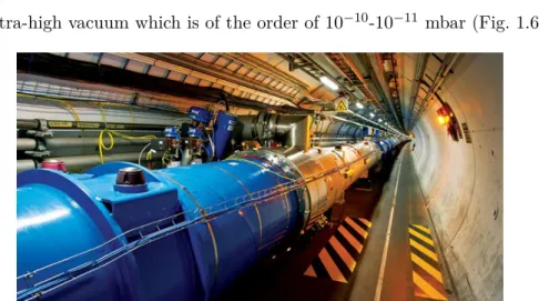
The LHC is the world’s largest and most powerful particle accelerator [CERN 2015]. It consists of 27 km of superconducting magnets and accelerating structures which increase the energy of particles. The accelerated particles move, in opposite direction, inside tubes kept at a ultra-high vacuum which is of the order of 10−10-10−11 mbar (Fig. 1.66).
Figure 1.6: A section of the LHC, the world’s largest particle accelerator.
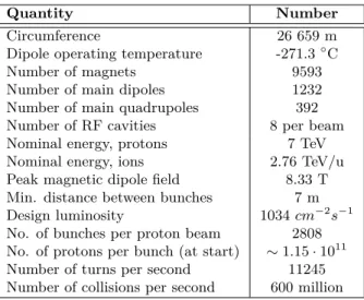
Tab. 1.1 [Lefevre 2009] lists the most important parameters for the LHC as the luminosity7, the nominal energy and the number of bunches (which are groups of particles in the accelerator space).
Among other facilities, the accelerator complex includes the Antiproton Decelerator (AD) providing low-energy antiprotons for the study of antimatter, the Linac 3, which is the starting point for the acceleration of heavy ions (Pb82+) and the neutron Time-of-Flight
6
©2013-2015 CERN.
http://home.web.cern.ch/topics/large-hadron-collider, 7 October 2015.
7
The luminosity L is the factor of proportionality between the event rate R in a collider and the interaction cross section σint: R = Lσint. If two bunches containing n1 and n2 particles collide with
frequency f , the luminosity is given by:
L = f n1n2 4πσxσy
Table 1.1: Main parameters of the LHC.
Quantity Number
Circumference 26 659 m
Dipole operating temperature -271.3◦C
Number of magnets 9593
Number of main dipoles 1232
Number of main quadrupoles 392
Number of RF cavities 8 per beam
Nominal energy, protons 7 TeV
Nominal energy, ions 2.76 TeV/u
Peak magnetic dipole field 8.33 T
Min. distance between bunches 7 m
Design luminosity 1034 cm−2s−1
No. of bunches per proton beam 2808
No. of protons per bunch (at start) ∼ 1.15 · 1011
Number of turns per second 11245
Number of collisions per second 600 million
facility (nTOF), built to study neutron-nucleus interactions.
Other major project and experiments, presently undergoing at CERN, are NA61/SHINE, studying the properties of the production of hadrons in collisions of beam particles and nuclei (such as pions8, protons, beryllium, argon and xenon) with different targets, NA62 for the study of rare kaon9 decays and the COmmon Muon and Proton Apparatus for Structure and Spectroscopy (COMPASS) for studying the behaviour of the interactions quarks10-gluons11.
Finally, a short list of decommissioned facilities which have generated radioactive waste that is currently stored at CERN includes:
• the CERN neutrinos to Grand Sasso (CNGS), used for the study of the characteristics of neutrinos (operations ceased in 2012);
8
The exchanged particles that carry nuclear force are called mesons. The lightest of the mesons, the
π-meson or pion, is responsible for the major portion of the longer range part of the nucleon-nucleon
potential. There are three types of pions with electric charges +1, 0 and -1. Their spin is 0 and their rest energies are 139.6 MeV (for π±) and 135.0 MeV (for π0) [Krane 1987].
9Kaons or K mesons are a type of meson having the property of strangeness, which is a decay caracteristic
[Krane 1987].
10A hadron is a composite particle, made of elementary particles called quark, which are held together by
the strong force. There exist three families of hadrons: baryons (qqq), antibaryons (qqq) and mesons (qq) [Hecht 2007][Mazzoldi et al. 1998]. Example of hadrons are the proton and the neutron.
11The force between quarks can be modeled as an exchange force, mediated by the exchange of massless
![Figure 1.7: Example of horizontal phase space for a generic section of the LHC. Here γ ( s ) = [1 + α 2 ( s )] /β ( s )](https://thumb-eu.123doks.com/thumbv2/123doknet/14505379.720020/57.893.183.663.215.592/figure-example-horizontal-phase-space-generic-section-lhc.webp)