Optimizing the translation out-of-SSA with renaming constraints

HAL Id: hal-02102190

https://hal-lara.archives-ouvertes.fr/hal-02102190

HAL is a multi-disciplinary open access archive for the deposit and dissemination of sci-entific research documents, whether they are pub-lished or not. The documents may come from teaching and research institutions in France or abroad, or from public or private research centers.

L’archive ouverte pluridisciplinaire HAL, est destinée au dépôt et à la diffusion de documents scientifiques de niveau recherche, publiés ou non, émanant des établissements d’enseignement et de recherche français ou étrangers, des laboratoires publics ou privés.

constraints

Fabrice Rastello, F. de Ferrière, Christophe Guillon

To cite this version:

Fabrice Rastello, F. de Ferrière, Christophe Guillon. Optimizing the translation out-of-SSA with re-naming constraints. [Research Report] LIP RR-2005-34, Laboratoire de l’informatique du parallélisme. 2005, 2+26p. �hal-02102190�

Unit´e Mixte de Recherche CNRS-INRIA-ENS LYON-UCBL no5668

Optimizing the translation out-of-SSA with

renaming constraints

Ecole Normale Sup´erieure de Lyon 46 All´ee d’Italie, 69364 Lyon Cedex 07, France

T´el´ephone : +33(0)4.72.72.80.37 T´el´ecopieur : +33(0)4.72.72.80.80 Adresse ´electronique :lip@ens-lyon.fr

constraints

Static Single Assignment form is an intermediate representation that uses φ instructions to merge values at each confluent point of the control flow graph. φ instructions are not machine instructions and must be renamed back to

move instructions when translating out of SSA form. Without a coalescing algorithm, the out of SSA translation generates many move instructions. Leung and George [8] use a SSA form for programs represented as native machine instructions, including the use of machine dedicated registers. For this purpose, they handle renaming constraints thanks to a pinning mechanism. Pinning φ arguments and their corresponding definition to a common resource is also a very attractive technique for coalescing variables. In this paper, extending this idea, we propose a method to reduce the φ-related copies during the out of SSA translation, thanks to a pinning-based coalescing algorithm that is aware of renaming constraints. This report provides also a discussion about the formulation of this problem, its complexity and its motivations. We implemented our algorithm in the STMicroelectronics Linear Assembly Optimizer [5]. Our experiments show interesting results when comparing to the existing approaches of Leung and George [8], Sreedhar et al. [11], and Appel and George for register coalescing [7].

Keywords: Static Single Assignment, Coalescing, NP-complete, K-COLORABILITY, Machine code level, register allocation

utilise des fonctions virtuelles φ pour fusionner les valeurs `a chaque point de confluence du graphe de contrˆole. Les fonctions φ n’existant pas physi-quement, elles doivent ˆetre remplac´ees par des instructions move lors de la translation en code machine. Sans coalesceur, la translation hors-SSA g´en`ere beaucoup demove.

Dans cet article, nous proposons une extention de l’algorithme de Leung et George [8] qui effectue la minimisation de ces instructions de copie. Leung et al. proposent un algorithme de translation d’une forme SSA pour du code assembleur, mais non optimis´e pour le remplacement des instructions φ. Par contre, ils utilisent la notion d’´epinglage pour repr´esenter les contraintes de renommage.

Notre id´ee est d’utiliser cette notion d’´epinglage afin de contraindre le renom-mage des arguments des φ pour faire du coalescing. C’est une formulation du probl`eme de coalescing non ´equivalente au probl`eme initial toujours consid´er´e comme ouvert dans la litt´erature [8,10]. Nous prouvons n´eanmoins la NP-compl´etude de notre formulation, une cons´equence de la preuve ´etant la NP-compl´etude du probl`eme initial en la taille de la plus grande fonction φ. Enfin, nous avons impl´ement´e notre algorithme dans le LAO [5], optimiseur d’assembleur lin´eaire. La comparaison avec diff´erentes approches possibles fournit de nombreux r´esultats int´eressants. Nous avons aussi essay´e, `a l’aide d’exemples faits `a la main, d’expliquer les avantages et limitations des diff´erentes approches.

Mots-cl´es: forme SSA, fusion de variables, NP-compl´etude, K-COLORABLE, code assembleur, allocation de registres

1

Introduction

Static Single Assignment The Static Single Assignment (SSA) form is an intermediate representation widely used in modern compilers. SSA comes in many flavors, the one we use is the pruned SSA form [4]. In SSA form, each variable name, or virtual register, corresponds to a scalar value and each variable is defined only once in the program text. Because of this single assignment property, the SSA form contains φ instructions that are introduced to merge variables that come from different incoming edges at a confluent point of the control flow graph. These φ instructions have no direct corresponding hardware instructions, thus a translation out of SSA must be performed. This transformation replaces φ instructions withmoveinstructions and some of the variables with dedicated ones when necessary. This replacement must be performed carefully whenever transformations such as copy propagation have been done while in SSA form. Moreover, a naive approach for the out of SSA translation generates a large number ofmove instructions. This paper1 addresses the problem of minimizing the number of generated copies during this translation phase.

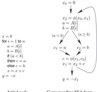
x0= 0 x2= φ(x0, x1) a = A[i] b = B[i] c = φ(c1, c2) x1= x2+ c (a ≥ b) c2= b c1= a (a < b) y = −x1 x = 0 fori = 1ton a = A[i] b = B[i] if(a < b) thenc = a elsec = b x = x + c y = −x

Initial code Corresponding SSA form

Figure 1: Example of code in non-SSA form and its corresponding SSA form without the loop counter represented

Previous Work Cytron et al. [4] proposed a simple algorithm that first replaces a φ instruction by copies into the predecessor blocks, then relies on Chaitin’s coalescing algorithm [3] to reduce the number of copies. Briggs et al. [1] found two correctness problems in this algorithm, namely the swap problem and the lost copy problem, and proposed solutions to these. Sreedhar et al. [11] proposed an algorithm that avoids the need for Chaitin’s coalescing algorithm and that can eliminate moremoveinstructions than the previous algorithms. Leung and George [8] proposed an out-of-SSA algorithm for an SSA representation at the machine code level. Machine code level representations add renaming constraints due to ABI (Application Binary Interface) rules on calls, special purpose ABI defined registers, and restrictions imposed on register operands.

1_{Many thanks to Alain Darte, Stephen Clarke, Daniel Grund and the reviewers of CGO for very helpful comments on} the presentation of this report.

Context of the study Our study of out-of-SSA algorithms was needed for the development of the STMicroelectronics Linear Assembly Optimizer (LAO) tool. LAO converts a program written in the Linear Assembly Input (LAI) language into the final assembly language that is suitable for assembly, linking, and execution. The LAI language is a superset of the target assembly language. It allows symbolic register names to be freely used. It includes a number of transformations such as induc-tion variable optimizainduc-tion, redundancy eliminainduc-tion, and optimizainduc-tions based on range propagainduc-tion, in an SSA intermediate representation. It includes scheduling techniques based on software pipelining and superblock scheduling, and uses a repeated coalescing [5] register allocator, which is an im-provement over the iterated register coalescing from George and Appel [7]. The LAO tool targets the ST120 processor, a DSP processor with full predication, 16-bit packed arithmetic instructions, multiply-accumulate instructions and a few 2-operands instructions such as addressing mode with auto-modification of base pointer.

Because of these particular features, an out-of-SSA algorithm aware of renaming constraints was needed. In fact, delaying renaming constraints after the out-of-SSA phase would result in additional

moveinstructions (see Section5), along with possible infeasibilities and complications. We modi-fied an out-of-SSA algorithm from Leung and George to handle renaming constraints and reduce the number ofmoveinstructions due to the replacement of φ instructions.

Layout of this paper The paper is organized as follows. Section2states our problem and gives a brief description of Leung and George’s algorithm. In Section3, we present our solution to the problem of register coalescing during the out-of-SSA phase. Section4discusses, through several examples, how our algorithm compares to others. In Section5, we present results that show the effectiveness of our solution on a set of benchmarks, and we finally conclude. This paper contains also two appendicesA

andBdevoted respectively to the refinement of Leung’s algorithm and to the NP-completeness proof of the pinning based coalescing problem.

2

Problem statement and Leung and George’s algorithm

Our goal is to handle renaming constraints and coalescing opportunities during the out of SSA transla-tion. For that, we distinguish dedicated registers (such as R0 or SP, the stack pointer) from general-purpose registers that we assume in an unlimited number (we call them virtual registers or variables). We use a pinning mechanism, in much the same way as in Leung and George’s algorithm [8], so as to enforce the use of these dedicated registers and to favor coalescing. Then, constraints on the number of general-purpose registers are handled later, in the register allocation phase.

2.1 Pinning mechanism

An operand is the textual use of a variable, either as a write (definition of the variable) or as a read (use in an instruction). A resource is either a physical register or a variable. Resource pinning or simply pinning is a pre-coloring of operands to resources. We call variable pinning the pinning of the (unique) definition of a variable. Due to the semantics of φ instructions, all arguments (i.e. use operands) of a φ instruction are pinned to the same resource as the variable defined (i.e. def operand) by the φ.

On the ST120 processor, as in Leung and George’s algorithm, we have to handle Instruction Set Architecture (ISA) register renaming constraints and Application Binary Interface (ABI) function parameter passing rules. Figure2, expressed in SSA pseudo assembly code, gives an example of such constraints. In this example and in the rest of this paper, the notation X ↑Ris used to mark that the

operand X is pinned to the resource R. When the use of a variable is pinned to a different resource than its definition, amoveinstruction has to be inserted between the resource of the definition and the resource of the use. Pinning the variable to the same resource as its uses has the effect of coalescing these resources (i.e., it deletes themove).

Original code: .input C, P load A, @P ++ load B, @P ++ call D = f (A, B) E = C + D K = 0x00A12BFA F = E − K .output F

SSA pinned code: Comments:

S0: .input C↑R0, P ↑P 0 Inputs C and P must be in R0 and P0 at the entry. S1:

½

load A, @P

autoadd Q↑Q, P ↑Q, 1

The second def. of P is renamed as Q in SSA, but P and Q must use the same resource for autoadd, e.g., Q.

S2: load B, @Q

S3: f D↑R0, A↑R0, B↑R1 Parameters must be in R0 and R1. Result must be in R0. S4: add E, C, D

S5: make L, 0x00A1

S6: more K↑K, L↑K, 0x2BFA Operands K & L must use the same resource, e.g., K. S7: sub F , E, K

S8: .output F ↑R0 Output F must be in R0.

Figure 2: Example of code with renaming constraints: function parameter passing rules (statements

S0, S3, and S8) and 2-operand instruction constraints (statements S1 and S6).

2.2 Correct pinning

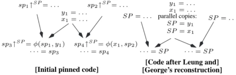
Figure3gives an example of renaming constraints that will result in an incorrect code. On the left of Figure3, the renaming constraint is that all variables renamed from the dedicated register SP (Stack Pointer) must be renamed back to SP, due to ABI constraints. On the right, after replacement of the φ instructions, the code is incorrect. Such problem mainly occurs after optimizations on dedicated registers: SSA optimizations such as copy propagation or redundancy elimination must be careful to maintain a semantically correct SSA code when dealing with dedicated-register constraints. More details on correctness problems related to dedicated registers are given in AppendixA.

y1= . . .

x1= . . .

y1= . . .

x1= . . .

parallel copies: _{SP = . . .}

[Code after Leung and]

sp3↑SP= φ(sp1, y1) · · · = sp3 · · · = SP ř ř ř ř SP = ySP = x11 sp4↑SP= φ(x1, sp2) · · · = sp4 · · · = SP

[Initial pinned code] [George’s reconstruction]

sp1↑SP= . . . sp2↑SP= . . .

SP = . . .

Figure 3: A too constrained pinning can lead to an incorrect code as for the parallel copies here. Cases of incorrect pinning are given in Figure5. In this figure, Case 1 and Case 2 are correct if and only if x and y are the same variable. This is because two different values cannot be pinned to a unique resource if both of them must be available at the entry point of an instruction (Case 2) or at the exit point of an instruction (Case 1). A similar case on φ instructions is given in Case 3: the set of φ instructions at a block entry has a parallel semantics, therefore two different φ definitions in the same block cannot be pinned to the same resource. On the other hand, on most architectures, Case 4 is a correct pinning. But, the corresponding scheme on a φ instruction (Case 5) is forbidden when s 6= r: this is because all φ arguments are implicitly pinned to the resource the φ result is pinned to. The

motivation for these semantics is given in AppendixA. Finally, Case 6 corresponds to a more subtle incorrect pinning, similar to the problem stressed in Figure3.

returnR0 R0 = x0 3 y2= y1+ K x4↑R0= g(x3↑R0, y2↑R1) y1↑R1= φ(y0, x2) returnx3↑R0

[Resulting out-of-SSA code] [Initial pinned SSA code]

R0 = g(R0, R1) R0 += 1 x0 3= R0 y2= R1 + K R1 = y2 x2↑R0= x0↑R0+1 x3↑R0= φ(x0, y0) ř ř ř ř R0 = R1_{R1 = R0} inputR0, R1 inputx0↑R0, y0↑R1

[Before mark phase] [After rename phase]

Figure 4: Transformation of already pinned SSA code by Leung and George’s algorithm.

y1= · · ·

x1= · · ·

L1:

Case 5: x↑r= φ(· · · y↑s_{· · · )}

Case 1: (x↑r, y↑r_{) = instr(...)}

Case 2: ... = instr(x↑r, y↑r₎

Case 3: ř ř ř ř x↑ r_{= φ(...)} y↑r_{= φ(...)} Case 4: x↑r= instr(y↑r₎ Case 6: x↑r_{= (x} 1, · · · ) y↑r_{= (· · · , y} 1)

Figure 5: All but Case 4 are incorrect pinning.

2.3 Leung and George’s algorithm

Leung and George’s algorithm is decomposed into three consecutive phases: the collect phase col-lects information about renaming constraints; the mark phase colcol-lects information about the conflicts generated by renaming; the reconstruct phase performs renaming, inserts copies when necessary and replaces φ instructions.

Pinning occurs during the collect phase, and then the out of SSA translation relies on the mark and reconstruct phases. Figure4illustrates the transformations performed during those last two phases:

• x₃is pinned to R0 on its definition. But, on the path to its use in thereturn, x4is also pinned to R0 on the call to g. We say that x3 is killed, and a repair copy to a new variable x03 is introduced.

• The use of x3 in the call to g is pinned to R0, while x3 is already available in R0 due to a prior pinning on the φ instruction. The algorithm is careful not to introduce a redundantmove

instruction in this case.

• The copies R0 = R1; R1 = R0 are performed in parallel in the algorithm, so as to avoid the so-called swap problem. To sequentialize the code, intermediate variables may be used and the copies may be reordered, resulting in the code t = R1; R1 = R0; R0 = t in this example.

Now, consider the non-pinned variable y2of Figure4and its use in the definition of x4. The use is pinned to a resource, R1, and y2 could have been coalesced to R1without creating any interference. The main limitation of Leung and George’s algorithm is its inability to do so. The same weakness shows up on φ arguments, as illustrated by Figure6(a): on a φ instruction X = φ(x0, . . . , xn), each

operand xi is implicitly pinned to X, while the definition of each xi may not. Our pinning-based

coalescing is an extension to the pinning mechanism whose goal is to overcome this limitation. 2.4 The φ coalescing problem

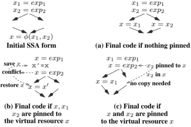
As opposed to the pinning due to ABI constraints, which is applied to a textual use of an SSA variable, the pinning related to coalescing is applied only to variable definitions (variable pinning). Figure6

illustrates how this pinning mechanism can play the role of a coalescing phase by preventing the re-construction phase of Leung and George’s algorithm from insertingmoveinstructions: in Figure6(b), x1 and x2 were pinned to x to eliminate thesemoveinstructions; however, this pinning creates an interference, which results in a repairmovex0= x along with amovex = x0on the replacement of the φ instruction; in Figure6(c), to avoid the interference, only x2was pinned to x, resulting in only onemoveinstruction.

(b) Final code if x, x1

the virtual resource x

x2are pinned to

x1= exp1

x2= exp2

x = φ(x1, x2)

Initial SSA form

x = exp1 x = exp2 x’=x conflict save x restore x _{x = x}0 x2= exp2 x1= exp1 x = x1 x = x2 x = exp2 x1= exp1 x2pinned to x x = x1 x2in x no copy needed (c) Final code if

x and x2are pinned to the virtual resource x (a) Final code if nothing pinned

Figure 6: Inability of Leung and George’s algorithm to coalesce x = x1and x = x2 instructions (a) ;

a worst (b) and a better (c) solution using variable pinning of x1and x2.

Therefore, we will only look for a variable pinning that does not introduce any new interference. In this case, for a φ instruction X = φ(x0, . . . , xn), we say that the gain for φ is the number of

indices i such that the variable xi is pinned to the same resource as X. Hence, our φ coalescing

problem consists of finding a variable pinning, with no new interference (i.e., without changing the number of variables for which a repair move is needed), that maximizes the total gain, taking into account all φ instructions in the program.

Algorithm 1 Main phases of our algorithm.

Program pinning(CFG Program P)

foreach basic block B in P, in an inner to outer loop traversal Initial G=Create affinity graph(B)

PrePruned G=Graph InitialPruning(Initial G) Final G=BipartiteGraph pruning(PrePruned G) PrunedGraph pinning(Final G)

3

Our solution

The φ coalescing problem we just formulated is NP-complete (see AppendixBfor details). Instead of trying to minimize the gain for all φ instructions together, our solution relies on a sequence of local optimizations, each one limited to the gain for all φ instructions defined at a confluence point of the program. These confluence points are traversed based on an inner to outer loop traversal, so as to optimize in priority the most frequently executed blocks. The skeleton of our approach is given in Algorithm1.

Let us first describe the general ideas of our solution, before entering the details. For an SSA variable y, we define y = Resource def(y) as r if the definition of y is pinned to r, or y otherwise. Also, for simplicity, we identify the notion of resource with the set of variables pinned to it. For a given basic block, we create what we call an affinity graph. Vertices represent resources; edges represent potential copies between variables that can be coalesced if pinned to the same resource. Edges are weighted to take into account interferences between SSA variables; then the graph is pruned (deleting in priority edges with large weights) until, in each resulting connected component, none of the vertices interfere: they can now be all pinned to the same resource. The rest of this section is devoted to the precise description of our algorithm. A pseudo code is given in Algorithm2on page 17. The consecutive steps of this algorithm are applied on the example of Figure8.

3.1 The initial affinity graph

For a given basic block, the affinity graph is an undirected graph where each vertex represents either a variable or its corresponding resource (if already pinned): two variables that are pinned to the same resource are collapsed into the same vertex. Then, for each φ instruction X = φ(x1, . . . , xn) at the

entry of the basic block, there is an affinity edge, for each i, 0 ≤ i ≤ n, between the vertex that contains X and the vertex that contains xi.

3.2 Interferences between variables

We define below four classes of interferences that can occur when pinning two operands of a φ instruc-tion to the same resource. We differentiate simple interferences from strong interferences: a strong interference generates an incorrect pinning. On the other hand, a simple interference can always be repaired despite the fact that the repair might generate additional copies. The goal is then to minimize the number of simple interferences and to avoid all strong interferences. The reader may find useful to refer, for each class, to Figure7.

[Class 1] Consider two variables x and y. If there exists a point in the control flow graph where both x and y are alive, then x and y interfere. Moreover, considering the definitions of x and y, one dominates the other (this is a property of the SSA form). If the definition of x dominates the definition of y, we say that the definition of x is killed by y. The consequence is that pinning the definitions of x and y to a common resource would result in a repair of x (as in Leung and George’s technique).

[Class 2] Consider a φ instruction y = φ(. . . , z, . . .) in basic block B. Let C be the block where the argument z comes from; textually, the use of z appears in block B (and is implicitly pinned to y), but semantically, it takes place at the end of basic block C (this is where amove instruction, if needed, would be placed). If x 6= z and x is live-out of block C, then x and the use of z interfere and we say that the definition of x is killed by y. Note our definition of liveness: a φ instruction does not occur where it textually appears, but at the end of each predecessor basic block instead. Hence, if not

used by another instruction, z would be treated as dead at the exit of block C and at the entry of block B.

[Class 3] Consider two variables x and y, both defined by φ instructions, but not necessarily in the same basic block. Some of their respective arguments (for example xiand yj) may interfere in a

common predecessor block B. In this case, we say that the definitions of x and y strongly interfere: indeed, as explained in Section2.2, pinning those two definitions together is incorrect.

[Class 4] Consider φ instructions y = φ(y1, . . . , yn) and z = φ(y1, . . . , yn), in the same basic

block and with the same arguments. Because of Leung and George’s repairing implementation, they cannot be considered as identical and we need to consider that they strongly interfere. Notice that a redundancy elimination algorithm should have eliminated this case before. Note that, by definition of Classes 3 and 4, all variables defined by φ instructions in the same basic block strongly interfere.

Also, we consider that variables pinned to two different physical registers strongly interfere.

y kills x

[Class 1] [Class 2]

y kills x

y = φ(y1, y2) z = φ(y1, y2) x strongly interferes with y y strongly interferes with z

[Classes 3 & 4] x = . . . y = . . . .. . x26= y1 . . . x = . . . z 6= x y = φ(., z) . . . = x x = φ(., x2)

Figure 7: Different kind of interferences between variables.

x2 class1 class2 x1 X2 x1 X2 0 A = {x1, X2} X1= φ(x2, x1) X3= φ(x2, x3) X1 x2 x3 X3 0 0 0 {x1, X2} = A A = {x1, X2, X1} B = {x3, x2, X3} X1 x2 x3 X3 0 class1 class3 1 2 1 {x1, X2} = A Initial G=PrePruned G: _{A = . . .} B = . . . {x1is in A, x2in B} . . . . . . Step 1: coalescing of L1: x1↑A= . . . x2↑B= . . . x3↑B= . . . X2↑A= φ(x1, x2) X1↑A= φ(x2, x1) X3↑B= φ(x2, x3) Initial G: PrePruned G=Final G: Resources: x2= . . . . . . . . . x3= . . . L2: x1↑A= . . . X2↑A= φ(x1, x2) Resources: Final G:

Step 2 (final): coalescing of L2: Pinned SSA code after step 1:

Initial SSA code: Pinned SSA code after step 2:

Final code: x2= . . . . . . x1= . . . X2= φ(x1, x2) . . . x3= . . . X1= φ(x2, x1) X3= φ(x2, x3) L1: B = . . . A = B . . . {x2is in A} {x3is in B} {X2is in A} {X1is in A, X3in B}

Figure 8: Program pinning on an example. Control-flow graphes are represented for code, with control-flow edges between basic blocks represented with solid black arrows. Affinity graphes are represented for step 1 and 2, with affinity edges represented as dashed gray lines, annotated with a weight, and with interferences edges represented as full gray lines, annotated with the class of the interference.

3.3 Interferences between resources

After the initial pinning (taking into account renaming constraints), a resource cannot contain two variables that strongly interfere. However, simple interferences are possible; they will be solved by Leung and George’s repairing technique. During our iterative pinning process, we keep merging more and more resources, but we make sure not to create any new interference. We say that two resources A = {x1, . . . , xn} and B = {y1, . . . , ym} interfere if pinning all the variables {x1, . . . , xn} and

{y1, . . . , ym} together creates either a new simple interference, or a strong interference, i.e., if there

exist xi and yj that interfere. This check is done by the procedureResource interfere; it uses the

procedure Resource killed that gives, within a given resource, all the variables already killed by another variable.Resource killedis given in a formal description, but obviously the information can be maintained and updated after each merge.

3.4 Pruning the affinity graph

The pruning phase is based on the interference analysis between resources. More formally, the op-timization problem can be stated as follows. Let G = (V, EAffinity) be the graph obtained from Create affinity graph(as explained in Section3.1): the set V is the set of vertices labeled by re-sources and EAffinityis the set of affinity edges between vertices. The goal is to prune (edge deletion) the graph G into G0 = (V, Epinned) such that:

Condition 1: the cardinality of Epinnedis maximized;

Condition 2: for each pair of resources (v1, v2) ∈ V2 in the same connected component of G0, v₁ and v2do not interfere, i.e.,Resource interfere(v1,v2) = false.

In other words, the graph G is pruned into connected components such that the total number of deleted edges from EAffinityis minimized and no two resources within the same connected component interfere.

First, because of Condition 2, all edges (v1, v2) in EAffinity such that v1 and v2 interfere need to be removed from G. The obtained graphPrePruned Gis bipartite. Indeed, let {Xi}1≤i≤m, with Xi = φ(xi,1, . . . , xi,n), be the set of φ instructions of the current basic block B. There are two kinds of

vertices in G, the vertices for the definitions VDEF S = {Resource def(Xi)}1≤i≤mand the other ones, for the arguments not already in VDEF S, VARGS = {Resource def(xi,j)}1≤i≤m, 1≤j≤n\ VDEF S. By

construction, there is no affinity edge between two elements of VARGS. Also, because elements of

VDEF S strongly interfere together, there remains no edge between two elements of VDEF S. Thus, G

is indeed bipartite.

Unfortunately, even for a bipartite affinity graph, the pruning phase is NP-complete in the number of φ instructions (see AppendixB). Therefore, we use a heuristic algorithm based on a greedy pruning of edges, where edges with large weights are chosen first. The weight of an edge (x, y) is the number of neighbors of x (resp. y) that interfere with y (resp. x). This has the effect of first deleting edges that are more likely to disconnect more interfering vertices (see details in the procedure Bipartite-Graph pruning). Note that, in the particular case of a unique φ instruction, this is identical to the “Process the unresolved resources” of the algorithm of Sreedhar et al. [11].

3.5 Merging the connected components

Once the affinity graph has been pruned, the resources of each connected component can be merged. We choose a reference resource in this connected component, either the physical resource if it exists (in this case, it is unique since two physical resources always interfere), or any resource otherwise. We change all pinnings to a resource of this component into a pinning to the reference resource. Finally,

we pin each variable (i.e., its definition) in the component to this reference resource. The correctness of this phase is insured by the absence of any strong interference inside the new merged resource. A formal description of the algorithm is given by the procedurePrunedGraph pinning. In practice, the update of pinning need be performed only once, just before the mark phase, so requiring only one traversal of the control flow graph. Also note that the interference graph can be built incrementally at each call toResource interfereand updated at each resource merge, using a simple vertex-merge operation: hence, as opposed to the merge operation used in the iterated register coalescing algo-rithm [7] where interferences have to be recomputed at each iteration, here each vertex represents a SSA variable and merging is a simple edge union.

We point out that, after this phase, our algorithm relies on the mark and reconstruct phases of Le-ung and George’s algorithm. But we use several refinements, whose details are given in AppendixA.

4

Theoretical discussion

We now compare our algorithm with previous approaches, through hand crafted examples.

4.1 Our algorithm versus register coalescing

The out-of-SSA algorithm of Briggs et al. [1] relies on a Chaitin-style register coalescing to remove

moveinstructions produced by the out of SSA translation. ABI constraints for a machine code level intermediate representation can be handled after the out of SSA translation by insertion of move

instructions at procedure entry and exit, around function calls, and before 2-operand instructions. However, several reasons favor combined processing of coalescing and ABI renaming during the out-of-SSA phase:

[CC1] SSA is a higher level representation that allows a more accurate definition of interferences. For example (see Figure9), it allows partial coalescing, i.e., the coalescing of a subset of the variable definitions. R0 = f3 r3= R0 R0 = w {z is in R0} · · · = R0 R0 = f2 R0 = f1 R0 = f1 z = R0 R0 = fz = R02 · · · = z R0 = f3 · · · = r · · · = r3

[Initial code] [Partially coalesced code]

z = w

Figure 9: Because the physical register R0 and z interfere, [Initial code] cannot be coalesced by Chaitin’s register coalescing; even if the three definitions of R0 are constrained to be done on R0 (and then even in SSA “R0” and “z” interfere), the pinning mechanism allows z and R0 to be coalesced, we say partially.

[CC2] The classical coalescing algorithm is greedy, so it may block further coalescings. Instead, for each merging point of the control flow graph, our algorithm optimizes together the set of coalescing opportunities for the set of φ instructions of this point.

[CC3] The main motivation of Leung and George’s algorithm is that ABI constraints introduce many additionalmove instructions. Some of these will be deleted by a dead code algorithm, but most of them will have to be coalesced. An important point of our method is the reduction of the overall complexity of the out-of-SSA renaming and coalescing phases: as explained in Section3.5,

the complexity of the coalescings performed under the SSA representation benefits from the static single definition property.

4.2 Our algorithm versus the algorithm of Sreedhar et al.

The technique of Sreedhar et al. [11] consists in first translating the SSA form into CSSA

(Conven-tional SSA) form. In CSSA, it is correct to replace all variable names that are part of a common φ

instruction by a common name, then to remove all φ instructions. To go from SSA to CSSA however, we may create new variables and insertmoveinstructions to eliminate φ variable interferences that would otherwise result in an incorrect program after renaming. Sreedhar et al. propose three algo-rithms to convert to CSSA form. We only consider the third one, which uses the interference graph and some liveness information to minimize the number of generatedmoveinstructions. Figures10-12

illustrate some differences between the technique of Sreedhar et al. and ours.

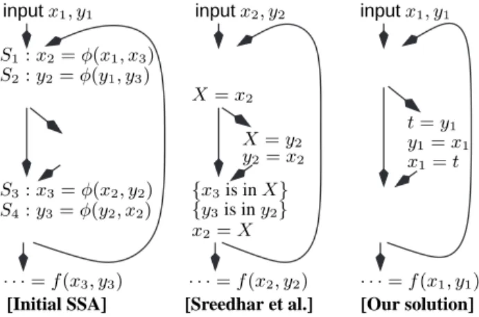
[CS1] Sreedhar et al. optimize separately the replacement of each φ instruction. Our algorithm considers all the φ instructions of a given block to be optimized together. This can lead to a better solution as shown in Figure10.

x = f1 y = f2

x = f1

z = f3

[Initial SSA] [Sreedhar et al.] [Our solution] [Solution of] S1: X = φ(x, y) S2 : Y = φ(z, y) Y = f3 X = x Y = X Y = f3 X = Y X = f1 Y = f2 X = f2

Figure 10: Sreedhar et al. treat S1 and S2 in sequence: for S1, {x, y} interfere so X = x is inserted

and {y, X} are regrouped in the resource X; for S2, {z, X} interfere so Y = X is inserted and

Y = {z, Y }. y2= x2 inputx2, y2 X = x2 x2= X X = y2 {x3is in X} {y3is in y2} inputx1, y1 S1: x2= φ(x1, x3) S2: y2= φ(y1, y3) S3: x3= φ(x2, y2) S4: y3= φ(y2, x2) inputx1, y1 t = y1 y1= x1 x1= t · · · = f (x3, y3) · · · = f (x2, y2) · · · = f (x1, y1)

[Initial SSA] [Sreedhar et al.] [Our solution]

Figure 11: The superiority of using parallel copies. For the solution of Sreedhar et al. we suppose

[CS2] Sreedhar et al. process iteratively modify the initial SSA code by splitting variables. By do-ing so, information on interferences becomes scattered and harder to use. Thanks to pinndo-ing, through-out the process we are always reasoning on the initial SSA code. In particular, as illustrated by Figure11, we can take advantage of the parallel copies placement.

[CS3] Finally, because our SSA representation is at machine level, we need to take into account ABI constraints. Figure12shows an example where we make a better choice of which variables to coalesce by taking the ABI constraints into account.

b0= f1 b1= φ(b0, B) b2= b1+ 1(autoadd) a = · · · a = · · · B = f1 B = f1 {b1is in B} b2= B + 1(autoadd) B = · · · {a is in B} L1: L2: B = b2 B = a [Our solution] B = φ(a, b2)

[Initial SSA] [Sreedhar et al.]

B+ = 1

Figure 12: {a, b2} interfere: without the ABI constraints information, adding themoveon block L1

or L2 is equivalent. Sreedhar et al. may make the wrong choice: treating the ABI afterward would

replace the autoadd into B = B + 1 ; b2 = B (because {B, b2} interfere) resulting in one moremove.

4.3 Limitations

Below are several points that expose the limitations of our approach:

[LIM1] Our algorithm is based on Leung and George’s algorithm that decides the place where moveinstructions are inserted. Also, we use an approximation of the cost of an interference compared to the gain of a pinning. Hence, even if we could provide an optimal solution to our formulation of the problem, this solution would not necessarily be an optimal solution for the minimization ofmove

instructions.

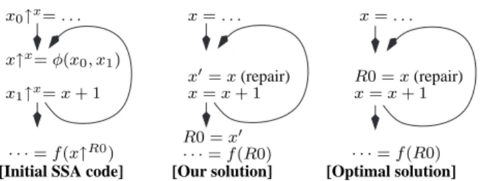
[LIM2] As explained in Section2.3, the main limitation of Leung and George’s algorithm is that, when the use of a variable is pinned to a resource, it does not try to coalesce its definition with this resource. This can be avoided by using a pre-pass to pin the variable definitions. But, as illustrated by Figure13, repairing variables that are introduced during Leung and George’s repairing phase cannot be handled this way.

[LIM3] As explained in AppendixB, our φ coalescing problem is NP-complete. Note also that a simple extension of the proof shows the NP-completeness of the problem of minimizing the number ofmoveinstructions.

[LIM4] Finally, in the case of strong register pressure, the problem becomes different: coalescing (or splitting) variables has a strong impact on the colorability of the interference graph during the register allocator phase (e.g. [9]). But this goes out of the scope of this paper.

R0 = x0 · · · = f (R0) x↑x_{= φ(x} 0, x1) x1↑x= x + 1 · · · = f (x↑R0₎ x0↑x= . . .

[Initial SSA code]

x0_{= x (repair)} x = x + 1 x = . . . [Our solution] x = x + 1 R0 = x (repair) · · · = f (R0) x = . . . [Optimal solution]

Figure 13: Limitation of Leung and George’s repairing process: the repairing variable x0 is not coa-lesced with further uses.

5

Results

We conducted our experiments on several benchmarks represented in LAI code. Since the LAI lan-guage supports predicated instructions, the LAO tool uses a special form of SSA, named ψ-SSA [13], which introduces ψ instructions to represent predicated code under SSA. In brief, ψ instructions in-troduce constraints similar to 2-operands constraints, and are handled in our algorithm in a special pass where they are converted into a “ψ-conventional” SSA form. This does not change the results presented in this section.

In the following, VALcc1 and VALcc2 refer to the same set of C functions compiled into LAI code with two different ST120 C compilers. This set includes about 40 small functions with some basic digital signal processing kernels, integer Discrete Cosine Transform, sorting, searching, and string searching algorithms. The benchmarks example1-8 are small examples written in LAI code specifically for the experiment. LAI Large is a set of larger functions, most of which come from the efr 5.1.0 vocoder from the ETSI [6]. Finally, SPECint refers to the SPEC CINT2000 benchmark [12].

To show the superiority of our approach, we have implemented the following algorithms:

[Leung] The algorithm of Leung and George contains the collect, and the mark-reconstruct (say out-of-pinned-SSA) phases. For some reasons given further, the collect phase has been split into three parts, namely pinningSP (collect constraints related to the dedicated register SP), pinningABI

(collect remaining renaming constraints) and pinningφ(our algorithm). Each of these pinning phases

can be activated or not, independently.

[Sreedhar] The algorithm of Sreedhar et al. has been implemented with an additional pass, namely pinningCSSA. The pinningCSSA phase pins all the operands of a φ to a same resource, and allows the out-of-pinned-SSA phase to be used as an out-of-CSSA algorithm.

[NaiveABI] is an algorithm that adds when necessarymoveinstructions locally around renaming

constrained instructions. This pass can be used when the pinningABIpass has not been activated. [Coalescing] Finally, we have implemented a repeated register coalescer [5]. As for the iterated register coalescer it is a conservative coalescer when used during the register allocation phase. But, outside of the register allocation context like here, it is an aggressive coalescing that does not take care of the colorability of the interference graph.

As already mentioned in Section 2.2, coalescing variables constrained by a dedicated register like the SP register can generate incorrect code. Similarly, splitting the SSA web of such variables poses some problems. Hence, it was not possible to ignore those renaming constraints during the out-of-SSA phase and to treat them afterwards. That explains the differentiation we made between pinningSPand pinningABIpasses: we choose to always execute pinningSP. Also, we tried to modify the algorithm of Sreedhar et al. to support SP register constraints. However, our implementation still performs some illegal variable splitting on some codes: the final non-SSA code contains fewermove

instructions, but is incorrect. Such cases mainly occurred with SPECint, and thus the SPECint figures

for the experiments including the algorithm of Sreedhar et al. must be taken only as an optimistic approximation of the number ofmoveinstructions.

Experiments _{Sreedhar pinning}

CSSA pinning SP pinning ABI pinning φ out-of-pinned-SSA Nai v eABI Coalescing Lφ+C • • • • C • • • T able 2 Sφ+C • • • • • Lφ, ABI+C • • • • • Sφ+LABI+C • • • • • • LABI+C • • • • T able 3 C • • • • Lφ,ABI • • • • Sφ • • • • • T able 4 LABI • • •

Table 1: Details of implemented versions

Tables2-5compares the number of resultingmoveinstructions on the different out-of-SSA algo-rithms detailed in Table1. In particular, we illustrate here comparisons [CC1-3] and [CS1-3] exposed in Section4. In the tables, values with + or - are always relative to the first column of the table. Comparison without ABI constraints Table2compares different approaches when renaming con-straints are ignored. As explained above only non-SP register related concon-straints, which we improperly call ABI constraints, could be ignored in practice. Columns Sφ+C vs Lφ+C illustrate points [CS1-2].

Columns C vs Lφ+C illustrate points [CC1-2]. Point [CC1] is also illustrated by Sφ+C vs C. In those

experiments, our algorithm is better or equal in all cases, except for the SPECint benchmark with the algorithm of Sreedhar et al.. But Sφ+C are optimistic results as explained before. It shows the

superiority of our approach in the absence of ABI constraints. benchmark Lφ+ C C Sφ+C VALcc1 193 +59 +3 VALcc2 170 +44 +13 example1-8 14 +3 +3 LAI Large 438 +44 +48 SPECint 6803 +3135 -59

Table 2: Comparison ofmoveinstruction count with no ABI constraint.

Comparison with renaming constraints Table3 shows the variation in the number of move in-structions of various out-of-SSA register coalescing algorithms, when all renaming constraints are taken into account. Comparison of Sφ+LABI+C and LABI+C vs Lφ,ABI+C confirms points [CS3].

Column C shows the importance of treating the ABI with the algorithm of Leung et al.: manymove

instructions could not be removed by the dead code and aggressive coalescing phases. Our algorithm leads to lessmoveinstructions in all cases which shows the superiority of our approach with renaming constraints.

benchmark Lφ,ABI+C Sφ+LABI+C LABI+C C VALcc1 242 +7 +3 +386 VALcc2 220 +15 +29 +449 example1-8 15 +3 +3 +18 LAI Large 1085 +26 +62 +634 SPECint 23930 +413 +482 +38623

Table 3: Comparison ofmoveinstruction count with renaming constraints.

Compilation time Repeated register coalescing is an expensive optimization phase in terms of time and space; its complexity is proportional to the number ofmoveinstructions in the program. Almost all coalescings are handled by our algorithm during the out of SSA translation. As explained in [2] the creation and the maintenance of the interference graph is highly simplified under the SSA form. Hence, as mentioned in Point [CC3], the moremove instructions are handled at the SSA level, the lower is the compilation time for the overall coalescing. Table4gives an evaluation of the number of

moveinstructions that would remain after the out-of-SSA phase if only naive techniques were applied for the φ replacement (which we denote φmoves) and for the renaming constraints treatment (which we improperly call ABImoves). Hence, it gives an evaluation of the cost of running a repeated register coalescing after one simple SSA rename back phase. We did not provide timing figures for the overall out-of-SSA and register coalescing phase for the different experiments because our implementation is too experimental and not optimized enough to give usable results.

benchmark Lφ,ABI Sφ LABI

ABImoves φmoves

VALcc1 277 +593 +690

VALcc2 245 +926 +749

example1-8 16 +38 +34

LAI Large 1447 +4543 +6161

SPECint 36882 +249481 +260095

Table 4: Comparison ofmoveinstruction count before the repeated register coalescing phase.

Variations on our algorithm Table5compares small variations in the implementation of our algo-rithm. The base column reports weighted move count, wheremoveinstructions are given a weight equal to 5d, d being the nesting level, i.e. depth, of the loop themovebelongs to. 5dis an arbitrary

benchmark base depth opt pess

VALcc1 1109 +1 +4 +1484

VALcc2 877 +1 +8 +1716

example1-8 32 +0 +0 +4

LAI Large 17594 +60 +7 +22116

SPECint 1652065 -1798 +7258 +3038712

weight that corresponds to a static approximation where each loop would contain 5 iterations. Our first variation (depth) is based on the simple remark that in our initial implementation we prioritized the φ instructions according to their depth, instead of the depth of themove instructions they will generate. For this variation, we use a newCreate affinity graphprocedure (Algorithm3) with a depth constraint that calls Program pinning with decreasing depth. This leads to a very small improvement on SPECint and a small degradation for LAI Large. This result confirms the observation we made that affinity and interference graphs are not complex enough to motivate a global optimization scheme.

Our second (opt) and third (pess) variations use relaxed definitions of interferences, respectively

optimistic and pessimistic (Algorithm4). It is interesting to note that optimistic interferences only incur a relatively small increase in the number ofmoveinstructions while significantly reducing the complexity of the computation of the interference graph.

6

Conclusion

This paper presents a pinning-based solution to the problem of register coalescing during the out-of-SSA translation phase. We explain and demonstrate why considering φ instruction replacement and renaming constraints together results in an improved coalescing of variables, thus reducing the number of move instructions before instruction scheduling and register allocation. We show the superiority of our approach both in terms of compile time and number of copies compared to solutions composed of existing algorithms (Sreedhar et al., Leung and George, Briggs et al., repeated register coalescing). These experiments also show that the affinity and interference graphs are usually quite simple, which means that a global optimization scheme would bring very little improvement over our local approach. Finally, we implemented some small variations of our algorithm, and observed that an optimistic implementation of interferences still provides good results with a significant reduction in the complexity of the computation of the interference graph. During this work, we also improved slightly the mark and reconstruct phases of Leung and George’s algorithm, which we rely on.

References

[1] P. Briggs, K. D. Cooper, T. J. Harvey, and L. T. Simpson. Practical improvements to the con-struction and decon-struction of static single assignment form. Software – Practice and Experience, 28(8):859–881, July 1998.

[2] Z. Budimlic, K. Cooper, T. Harvey, K. Kennedy, T. Oberg, and S. Reeves. Fast copy coa-lescing and live-range identification. In SIGPLAN International Conference on Programming

Languages Design and Implementation, pages 25–32. ACM Press, June 2002.

[3] G. J. Chaitin. Register allocation & spilling via graph coloring. In Proceedings of the 1982

SIGPLAN symposium on Compiler construction, pages 98–101, 1982.

[4] R. Cytron, J. Ferrante, B. Rosen, M. Wegman, and K. Zadeck. Efficiently computing static single assignment form and the control dependence graph. ACM Transactions on Programming

Languages and Systems, 13(4):451 – 490, 1991.

[5] B. Dupont de Dinechin, F. de Ferri`ere, C. Guillon, and A. Stoutchinin. Code generator optimiza-tions for the ST120 DSP-MCU core. In International Conference on Compilers, Architecture,

[6] European Telecommunications Standards Institute (ETSI). GSM technical activity, SMG11 (speech) working group. Available athttp://www.etsi.org.

[7] L. George and A. W. Appel. Iterated register coalescing. ACM Transactions on Programming

Languages and Systems, 18(3), May 1996.

[8] A. L. Leung and L. George. Static single assignment form for machine code. In SIGPLAN

International Conference on Programming Languages Design and Implementation, pages 204 –

214, 1999.

[9] J. Park and S.-M. Moon. Optimistic register coalescing. In IEEE International Conference on

Parallel Architectures and Compilation Techniques, pages 196–204, 1998.

[10] M. Sassa, T. Nakaya, M. Kohama, T. Fukukoa, and M. Takahashi. Static Single Assignment form in the COINS compiler infrastructure.

[11] V. Sreedhar, R. Ju, D. Gillies, and V. Santhanam. Translating out of static single assignment form. In Static Analysis Symposium, Italy, pages 194 – 204, 1999.

[12] Standard Performance Evaluation Corporation (SPEC). SPEC CINT2000 benchmarks. Avail-able athttp://www.spec.org/cpu2000/CINT2000/.

[13] A. Stoutchinin and F. de Ferri`ere. Efficient static single assignment form for predication. In

34th annual ACM/IEEE international symposium on Microarchitecture, pages 172–181. IEEE

Computer Society, 2001.

[14] Y. Wu and J. R. Larus. Static branch frequency and program profile analysis. In MICRO –

International Symposium on Microarchitecture, pages 1–11, New York, NY, USA, 1994. ACM

Algorithm 2 Formal description of our algorithm.

Create affinity graph(CFG Node current node)

(E, V ) = (∅, ∅)

for eachX = φ(x1, . . . , xn)of current node V = VS{Resource def(X)}

for eachx ∈ {x1, . . . , xn} V = VS{Resource def(x)}

e = (Resource def(X),Resource def(x))

if (e 6∈ E) multiplicity(e)=0 E = ES{e}, multiplicity(e)++ returnG = (E, V )

Graph InitialPruning(Graph (V, E))

foreach(x1, x2) ∈ E,

if (Resource interfere(x1, x2)) E −= (x1, x2)

return(V, E)

BipartiteGraph pruning(Bipartite Multi Graph (V, E))

{Evaluates the weight for each edge} for alle ∈ E, weight(e)=0

for all((x, x1), (x, x2)) ∈ E2such thatx16= x2 if Resource interfere(x1, x2)

weight((x, x1))+=multiplicity((x, x2)) weight((x, x2))+=multiplicity((x, x1)) {Prunes in decreasing weight order

and update the weight} while weight(ep)> 0 letep= (X, x)such that

∀e ∈ E, weight(ep)≥weight(e) do

E −= ep

for alle = (X, y) ∈ E

weight(e)−=multiplicity(ep) for alle = (Y, x) ∈ E

weight(e)−=multiplicity(ep) return(V, E)

PrunedGraph pinning(Graph G, Program P)

foreachV ∈ {connected components of G} letu =S_v∈V v

letw =

½

vi ifvi∈ V is a physical resource

u otherwise

foreach(OP ) d1, · · · = instr(a1, . . . ) ∈ P foreachdisuch thatdi∈ u

pinditowin(OP ) foreachai↑rsuch thatr ∈ V

replacerbyw

Variable kills(Variable a, Variable b)

if the definition ofbdominates those ofa andaandbinterfere

return true{Case 1}

ifais defined asa = φ(a1: B1, . . . , an: Bn) fori = 1ton

ifbis live out ofBiandb 6= ai return true{Case 2} return false

Variable stronglyInterfere(Variable a, Variable b)

ifaandbare defined byφinstructions leta : Ba = φ(a1: Ba,1, . . . , an : Ba,n) letb : Bb= φ(b1: Bb,1, . . . , bm: Bb,m) ifBa= Bbreturn true{Case 4} fori = 1ton

ifBa,iis a predecessor ofBb letBa,i= Bb,j

ifai6= bj return true{Case 3} return false

else ifaandbare defined in the same instruction let(· · · a · · · b · · · ) =instr(· · · ) return true return false Resource killed(Resource A) letA = {a1, . . . , an} killed withinA =

{ai∈ A|∃aj∈ A, Variable kills(aj, ai)} returnkilled withinA

Resource interfere(Resource A, Resource B)

letA = {a1, . . . , an} letB = {b1, . . . , bm}

letkilled withinA =Resource killed(A)

letkilled withinB =Resource killed(B)

ifAandBare physical resources ifA 6= B return true

for all(a, b) ∈ A × B

ifa 6∈ killed withinAand Variable kills(b, a) return true

ifb 6∈ killed withinB and Variable kills(a, b) return true

if Variable stronglyInterfere(a, b) return true

Algorithm 3 Construction of initial affinity graph with a depth constraint.

Create affinity graph(CFG Node current node, Integer depth)

(E, V ) = (∅, ∅)

for eachX = φ(x1, . . . , xn)of current node V = VS{Resource def(X)} for eachx ∈ {x1, . . . , xn} let Nodex:x = . . . if depth(Nodex)6=depth continue V = VS{Resource def(x)}

e = (Resource def(X),Resource def(x))

if (e 6∈ E) multiplicity(e)=0 E = ES{e}, multiplicity(e)++ returnG = (E, V )

Algorithm 4 Optimistic and pessimistic definition of interferences.

Variable kills optimistic(Variable a, Variable b)

let Nodea: (Defa)a = . . . let Nodeb: (Defb)b = . . .

if(a 6= b)and (Def bdominates Def a) and

(b ∈liveout(Nodea))

return true{Case 1}

ifais defined asa = φ(a1: B1, . . . , an: Bn) fori = 1ton

ifbis live out ofBiandb 6= ai return true{Case 2} return false

Variable kills pessimistic(Variable a, Variable b)

let Nodea: (Defa)a = . . . let Nodeb: (Defb)b = . . .

if(a 6= b)and (Def bdominates Defa) and

((b ∈livein(Node a))or(Nodea =Nodeb)) return true{Case 1}

ifais defined asa = φ(a1: B1, . . . , an: Bn) fori = 1ton

ifbis live out ofBiandb 6= ai return true{Case 2} return false

Appendix A: Limitations and refinement of Leung’s algorithm

Once pinning has been performed, our algorithm relies on Leung’s mark and reconstruct algo-rithms to restore the code into non-SSA form. Critical edges are subject to a particular treatment in Leung’s algorithm. But as illustrated by Figure14, the solution is not robust enough when dealing with aggressive pinning. The goal of this appendix is to propose a clearest semantic for φ functions, and to modify Leung’s algorithm accordingly.

x1← expr1 r ← expr2 r1← ← r4 ← r2 r4← φ(r1, x1)

Original code SSA code with copies folded

riare pinned to r

Leung’s solution to replace

φ-functions is incorrect:

the inserted copy kills the previous definition of r. x ← expr1 r ← expr2 y ← r r ← x ← r ← y x1← expr1 r2← expr2 r ← x ← r ← r r ← r ←

Figure 14: The φ-function replacement conflict problem

To begin with, let us consider a φ definition B : y = φ(. . . ). The semantic used by Leung et al. is that this definition is distributed over each predecessor of B. Hence, in a certain sense multiple definitions of Y coexist and therefore may conflict. Because conflicts for simple variables (not resources) are not taken into account in Leung’s algorithm, the lost copy problem has a special treatment that corresponds to the lines below the“(*fix problem related to critical edge*)”. Here, the copy cp3 := cp3

S

{w ← z} is incorrect (probably a typo) and it is difficult to fix to obtain a correct and efficient code. Instead, that whenever the definition of y is not pinned to any resource, we propose to create a virtual resource y and to pin this definition to it. This fix takes place in theCOLLECT procedure.

Another consequence of Leung’s φ function semantic is that whenever y has to be repaired, the repairing copies are also distributed over each predecessors of B. Hence conflicts can occur and those repairing copies cannot be used further B (which explains the need to introduce another repairing copy w). Because we found no a priori motivation to do so, we propose to place the repairing copy of y just after its definition instead. Hence, our new semantic of a given B : y↑r= φ(x1 : B1, . . . , xn : Bn)

(where y is always pinned to a resource r) definition is the following:

• at the end of each block Bi, there is a new virtual instruction that defines no variable but that

uses xi↑r.

• at the beginning of the block B, the φ instruction contains no use arguments, but defines y↑r.

• all the “virtual uses” of the end of each block have a parallel semantic i.e. are considered all together.

The consequence is a simplification of the code: whenever instructions of a block have to be traversed then φ functions definitions, normal instructions uses, normal instructions definitions and φ functions uses (of each successors) are considered consecutively.

The refined code is given below, modified code is written using the . sign.

Finally, we would like to outline the problem with dedicated register pinning. Indeed, we could find in Leung’s collect phase the code “ifywas renamed from some dedicated registerrduring SSA construction thenmust def [y] = r...”. As illustrated by Figure15 copy-folding performed on dedicated register definition can lead to an incorrect pinning. Because of its non local property, this inconsistency is not trivial to detect while doing the optimization. Freezing optimizations when dealing with dedicated registers is a solution to this problem. On the other hand the semantic is not necessarily strict enough to justify such a decision and pinning may be performed correctly while be-ing aware of this specific semantic. Hence because dedicated registers related pinnbe-ing that is semantic aware can be very complex, we have intentionally removed this part from the COLLECT procedure and delegated it to a previous pinning phase.

← r r ← r ← x ← r y ← x ← r ← y r ← y1← r ← x1← r1 ← ← r3 ← r4 r4= φ(x1, r2) r2← r ← ← r ← r y1← x1← ř ř ř ř r ← y_{r ← x}1₁ parallel copies:

Original code SSA form after copy folding and

dead-code elimination (incorrect parallel copies)

r3= φ(r1, y1)

Code generated by the reconstruction algorithm of Leung and George

procedureCOLLECT

initialize all entries ofmust defandmust useto⊥

R :=∅

forb∈basic blocksdo

fori∈ φ-functions inb do

let i ≡ y ← φ(x1. . . xn)

. if pinned def (i, 1)

. then let rbe the dedicated register required

. else let r = y must def [y] = r

R := R∪{r}

fori∈non-φ-functions inb do

let i ≡ y1. . . ym← op(x1. . . xn)

for j := 1 to m do if pinned def (i, j) then

let rbe the dedicated register required

must def [yj] := r

R := R∪{r}

for j := 1 to n do if pinned use(i, j) then

let rbe the dedicated register required

must use[i][j] := r

R := R∪{r}

procedureMARKINIT

forb∈basic blocksdo

for r ∈Rdo sites[r] := ∅ forr∈Rdo

last[b][r] := > phi[b][r] := >

fori∈ φ-functions in blockb do

let i ≡ y ← φ(x1. . . xn)

if must def [y] = r 6= ⊥ then phi[b][r] = last[b][r] = y sites[r] := sites[r] ∪ {b}

fori∈normal instructions in blockb do

let i ≡ y1. . . ym← op(x1. . . xn)

forj := 1to n do

if must use[i][j] = r 6= ⊥ then last[b][r] := xj

sites[r] := sites[r] ∪ {b}

forj := 1 tom do

if must def [yj] = r 6= ⊥ then

last[b][r] := yj

sites[r] := sites[r] ∪ {b} . forb’∈ succcf g(b) do

. let bbe thejth predecessor ofb0

. for i ∈ φ-functions inb0_do

. let r ≡ must def [y] . last[b][r] = xj . sites[r] := sites[r] ∪ {b} procedureMARK MARKINIT() forr∈Rdo repair name[r] = ⊥ repair sites[r] = ∅ for b ∈basic blocksdo

forr∈Rdo

avail[r] := avin[b][r]

fori∈normal instructions inb do

let i ≡ y1. . . ym← op(x1. . . xn)

forj := 1to n do USE(i, j, xj)

forj := 1to m do DEFINE(yj)

forb’∈ succcf g(b) do

let bbe thejth predecessor ofb0

for i∈ φ-functions inb0 do let i ≡ y ← φ(. . . xj. . .) USE(i, j, xk) avout[b][r] = ½ x if last[b][r] = x 6= > avin[b][r] otherwise

procedureUSE(i, j, x)

in place[i][j] = f alse

if must use[i][j] 6= ⊥ and avail[must use[i][j]] = x then in place[i][j] = true

return

if must def [x] 6= ⊥ and avail[must def [x]] 6= x then if repair name[x] = ⊥ then

repair name[x]:= a new SSA name

repair sites[x] := repair sites[x] ∪ {i} if must use[i][j] 6= ⊥ then

avail[must use[i][j]] := x procedureDEFINE(x)

if must def [x] 6= ⊥ then avail[must def [x]] := x

avin[b][r] =        ⊥ if b is the entry x if phi[i][r] = x 6= top T

b0_{∈predcf g(b)}avout[b0][r]if b ∈ DF+(sites[r])

procedureLOOKUP(i, x) if stacks[x]is emptythen

if must def [x] 6= ⊥ then return must def [x] else return x

else

let (y, sites) = top(stacks[x]) if i ∈ sites then return y

else if must def [x] 6= ⊥ then return must def [x] else return x

procedureRENAME USE(i, j, x, copies) let y =LOOKUP(i, x)

let r = must use[i][j] if in place[i][j] then

rewrite thejth input operand ofitor

else if r 6= ⊥ then

copies := copies ∪ {r ← y}

rewrite thejth input operand ofitor

else

rewrite thejth input operand ofitoy

return copies

procedureRENAME DEF(i, j, y, copies)

let r = if must def [y] = ⊥ then y else must def [y]

rewrite thejth output operandytor

if repair name[y] = tmp 6= ⊥ then

push(tmp, repair sites[y])ontostacks[y]

copies := copies ∪ {tmp ← r} return copies procedureRECONSTRUCT(b) fori∈ φ-functions inb do let i ≡ y ← φ(x1. . . xn) . cp4= ∅

. cp4= REN AM E DEF (i, 1, y, cp4)

. insert parallel copiescp4afteri

fori∈normal instructions inb do

(* rewrite instructions *)

let i ≡ y1. . . ym← op(x1. . . xn)

cp1:= ∅

forj := 1to n do

cp1:= REN AM E U SE(i, j, xj, cp1)

insert parallel copiescp1beforei

cp2:= ∅

forj := 1to m do

cp2:= REN AM E DEF (i, j, yj, cp2)

insert parallel copiescp2afteri

cp3:= ∅

(* computeφ-copies *)

forb’∈ succcf g(b) do

let bbe thekth predecessor ofb0

fori∈ φ-functions inb0

do let i ≡ y ← φ(x1. . . xk. . . xn)

. forj := 1to n do

. cp3:= REN AM E U SE(i, j, xj, cp3)

insert parallel copiescp3at the end of blockb

forb’∈ succdom(b) do

RECONSTRUCT(b0₎

Restorestacks[]to its state