Contributions to scientific computing for data-simulation interaction in biomedical applications

(1)

HAL Id: tel-03114756

https://hal.inria.fr/tel-03114756

Submitted on 19 Jan 2021

HAL is a multi-disciplinary open access archive for the deposit and dissemination of sci-entific research documents, whether they are pub-lished or not. The documents may come from teaching and research institutions in France or abroad, or from public or private research centers.

L’archive ouverte pluridisciplinaire HAL, est destinée au dépôt et à la diffusion de documents scientifiques de niveau recherche, publiés ou non, émanant des établissements d’enseignement et de recherche français ou étrangers, des laboratoires publics ou privés.

Contributions to scientific computing for

data-simulation interaction in biomedical applications

Damiano Lombardi

To cite this version:

Damiano Lombardi. Contributions to scientific computing for data-simulation interaction in biomed-ical applications. Modeling and Simulation. Sorbonne Université, 2020. �tel-03114756�

(2)

Contributions to scientific computing for

data-simulation interaction in biomedical applications.

Mémoire d’Habilitation à Diriger des Recherches

Damiano Lombardi

Presented on July, the 1st, 2020 in front of the jury:

Prof. Yvon Maday, Sorbonne Université, President

Prof. Fabio Nobile, EPFL, Reviewer

Prof. Karen Veroy, TU Eindhoven, Examiner

Prof. Stefan Volkwein, Konstanz University, Reviewer

Prof. Esther Pueyo, Zaragoza University, Examiner

Dir. Miguel Fernandez, Inria Paris, Examiner

(3)

List of Figures

1.1 Sequences of images, testcase presented in Section 1.1. . . 10 1.2 Evolution of a lung nodule, with slow dynamics, over 45 months. Test case

presented in Section 1.1 . . . 10 1.3 Example of a simulation of the 55 main arteries of the human body, Section 1.2.1. 12 1.4 Geometry of large arterioles, for the simulations discussed in Section 1.2.2: a)

global view of the mesh; b) map of the control points for the comparison with the experiment detailed in [RRG+86]. . . 14 1.5 Comparison to the experimental data, Section 1.2.2: the green markers represent

the values extracted in the control points for the 3D model, to be compared to the red markers obtained experimentally. . . 15 1.6 Result for the experiment commented in Section 1.2.3: velocity magnitude for the

target solution (left), the CFI data (center), reconstruction (right) . . . 17 1.7 (A) CMA-ES parameter calibration of the Courtemanche model prior to the

in-verse procedure. APs obtained for the most representative samples of the SR (blue) and AF (red) groups, reference parameters (dashed) and after AF remod-eling (dotted). (B) Courtemanche conductances estimated marginal densities for the SR (blue) and AF (red) groups. Conductances are normalized by the liter-ature values. (C) Normalized histograms of the four experimental biomarkers of interest for both SR (blue) and AF (red) groups. The black solid lines correspond to the PDF of each biomarker estimated by OMM. . . 20 1.8 Experimental data ternary classification results, Section 1.3.2. . . 23

2.1 Example of 3D two marginals optimal transport, Section 2.2.1: at the left %0, at

the right %1. . . 33

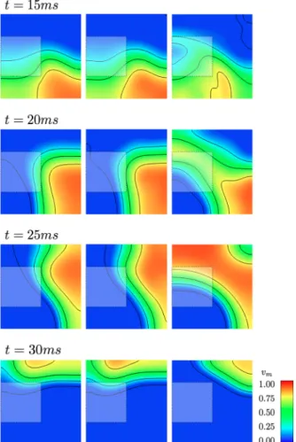
2.2 Simulation of the Monodomain equation, Section 2.3.2: left column, FEM solu-tion; in the center, the solution obtained by ALP; right column, POD solution. . 42 2.3 Evolution of the rank of the approximate solution for the 3D-3D Landau damping

test case as a function of time. . . 50 2.4 Fluctuations of density 1 ⇢(t, x) for the 3D-3D Landau damping test case at

times t = 0, 0.33, 0.67, 1.0 from left to right. . . 50 2.5 Vlasov-Poisson solution, section 2.4.2: (a) the tensor entries, in red the largest

entries; (b) the small size subtensors, (c) and (d) the mid size and the larger size subtensors. The largest subtensors are in the complement of the cube. . . 52 2.6 Vlasov-Poisson case, section 2.4.2: . . . 54

(6)

Author’s bibliography.

Ph.D. thesis: [22], Inverse Problems for tumour growth modeling, defended in Bordeaux on 09-09-2011.

Journal Articles:

• [4], Bakhta, A., Lombardi, D. (2018). An a posteriori error estimator based on shifts for positive hermitian eigenvalue problems. Comptes Rendus Mathematique, 356(6), 696-705. • [30], Tixier, E., Raphel, F., Lombardi, D., Gerbeau, J. F. (2018). Composite biomarkers derived from Micro-Electrode Array measurements and computer simulations improve the classification of drug-induced channel block. Frontiers in physiology, 8, 1096.

• [18], Gerbeau, J. F., Lombardi, D., Tixier, E. (2018). How to choose biomarkers in view of parameter estimation. Mathematical biosciences, 303, 62-74.

• [3], Aletti, M., Lombardi, D. (2017). A reduced-order representation of the Poincar´e-Steklov operator: an application to coupled multi-physics problems. International Journal for Numerical Methods in Engineering, 111(6), 581-600.

• [19], Gerbeau, J. F., Lombardi, D., Tixier, E. (2018). A moment-matching method to study the variability of phenomena described by partial di↵erential equations. SIAM Journal on Scientific Computing, 40(3), B743-B765.

• [29], Tixier, E., Lombardi, D., Rodriguez, B., Gerbeau, J. F. (2017). Modelling variability in cardiac electrophysiology: A moment-matching approach. Journal of the Royal Society Interface, 14(133), 20170238.

• [13], Ehrlacher, V., Lombardi, D. (2017). A dynamical adaptive tensor method for the Vlasov–Poisson system. Journal of Computational Physics, 339, 285-306.

• [2], Aletti, M., Gerbeau, J. F., Lombardi, D. (2016). A simplified fluid–structure model for arterial flow. application to retinal hemodynamics. Computer Methods in Applied Mechanics and Engineering, 306, 77-94.

• [1], Aletti, M., Gerbeau, J. F., Lombardi, D. (2016). Modeling autoregulation in three-dimensional simulations of retinal hemodynamics. Journal for Modeling in Ophthalmology, 1(1), 88-115.

• [25], Damiano Lombardi, Sanjay Pant. A non-parametric k-nearest neighbor entropy esti-mator. Physical Reviev E, 2016, 10.1103/PhysRevE.93.013310.

• [2], Matteo Aletti, Jean-Fr´ed´eric Gerbeau, Damiano Lombardi. A simplified fluid-structure model for arterial flow. Application to retinal hemodynamics. Computational Methods in Applied Mechanics and Engineering, 2016, 306, pp.77-94.

(7)

• [27], Sanjay Pant, Damiano Lombardi. An information-theoretic approach to assess prac-tical identifiability of parametric dynamical systems. Mathemaprac-tical Biosciences, Elsevier, 2015, pp.66-79.

• [24], Damiano Lombard, Emmanuel Maitre, E. (2015). Eulerian models and algorithms for unbalanced optimal transport. ESAIM: Mathematical Modelling and Numerical Analysis, 49(6), 1717-1744.

• [17], Jean-Fr´ed´eric Gerbeau, Damiano Lombardi, Elisa Schenone. Reduced order model in cardiac electrophysiology with approximated Lax pairs. Advances in Computational Mathematics, Springer Verlag, 2014, pp.28.

• [16], J.-F. Gerbeau, D.Lombardi. Approximated Lax pairs for the reduced order integration of nonlinear evolution equations, Journal of Computational Physics, 265; 246:269, 03-2014 • [21], Angelo Iollo, Damiano Lombardi. Advection modes by optimal mass transfer. Physical Review E : Statistical, Nonlinear, and Soft Matter Physics, American Physical Society, 2014, 89, pp.022923.

• [10] Thierry Colin, Francois Cornelis, Olivier Saut, Patricio Cumsille, Damiano Lombardi, et al.. In vivo mathematical modeling of tumor growth from imaging data : soon to come in the future?. Diagnostic and Interventional Imaging, Elsevier, 2013, pp.571-574.

• [23], Damiano Lombardi. Inverse problems in 1D hemodynamics on systemic networks: a sequential approach. International Journal for Numerical Methods in Biomedical Engi-neering, John Wiley and Sons, 2013

• [8], Damiano Lombardi, Angelo Iollo, Thierry Colin, Olivier Saut. Inverse Problems in tumor growth modeling by means of semiempirical eigenfunctions. Mathematical Models and Methods in Applied Sciences, World Scientific Publishing, 2012, pp.1.

• [20], Damiano Lombardi, Angelo Iollo. A Lagrangian Scheme for the Solution of the Optimal Mass Transfer Problem. Journal of Computational Physics, Elsevier, 2011, 230, pp.3430:3442.

(8)

Book section:

• [5], Michel Bergmann, Thierry Colin, Angelo Iollo, Damiano Lombardi, Olivier Saut, et al.. Reduced Order Models at work. Quarteroni, Alfio. Modeling, Simulation and Applications, 9, Springer, 2013.

• [9], T.Colin, A.Iollo, D.Lombardi, O.Saut, F.Bonichon and J.Palussire: Some models for the prediction of tumor growth: general framework and applications to metastases in the lung, Computational Surgery, Springer 2012.

Scientific popularization:

• [7], Thierry Colin, Angelo Iollo, Damiano Lombardi, Olivier Saut. Prediction of the Evo-lution of Thyroidal Lung Nodules Using a Mathematical Model. ERCIM News, ERCIM, 2012, 82, pp.37-38.

In revision/preparation:

• [14], Ehrlacher, V., Lombardi, D., Mula, O., Vialard, F. X. (2019). Nonlinear model reduc-tion on metric spaces. Applicareduc-tion to one-dimensional conservative PDEs in Wasserstein spaces. arXiv preprint arXiv:1909.06626.

• [12], Ehrlacher, V., Grigori, L., Lombardi, D., Song, H. (2019). Adaptive hierarchical subtensor partitioning for tensor compression. HAL:https://hal.inria.fr/hal-02284456 • [26], Lombardi, D., Raphel, F. (2019). A greedy dimension reduction method for

classifi-cation problems. HAL:https://hal.inria.fr/hal-02280502

• [28], Raphel, F., de Korte, T., Lombardi, D., Braam, S., Gerbeau, J. F. (2019). A greedy classifier optimisation strategy to assess ion channel blocking activity and pro-arrhythmia in hiPSC-cardiomyocytes. HAL:https://hal.inria.fr/hal-02276945

• [11], Alfonsi, A., Coyaud, R., Ehrlacher, V., Lombardi, D. (2019). Approximation of Opti-mal Transport problems with marginal moments constraints. arXiv preprint arXiv:1905.05663. • [15], Galarce, F., Gerbeau, J. F., Lombardi, D., Mula, O. (2019). State estimation with

nonlinear reduced models. Application to the reconstruction of blood flows with Doppler ultrasound images. arXiv preprint arXiv:1904.13367.

• Lombardi, D. Fast state estimation in time dependent systems: tensors and Kalman fil-tering.

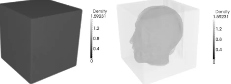
• Lombardi, D., Maday, Y. and Uro, L. A reduced basis approach for aided segmentation of facial muscles.

(9)

• [6], Cances, E., Ehrlacher, V., Gontier, D., Levitt, A., Lombardi, D. (2018). Numeri-cal quadrature in the Brillouin zone for periodic Schrodinger operators. arXiv preprint arXiv:1805.07144, in revision.

• Ratelade, J., Klug, N., Kaelle, M., Cruz, S. Debertrand, F., Domenga, V., Salman, R., Smith, C., Gerbeau, J.-F., Nelson, M., Joutel, A. Reducing hypermuscularization of the transitional segment between arterioles and capillaries protects against spontaneous intrac-erebral hemorrhage, in revision.

(10)

Introduction.

My research activity deals with scientific computing. In particular, the goal is to investigate numerical methods and algorithms to make data-simulation interaction feasible and efficient.

Two main axes can be identified: one, methodological, the other applied to the biomedical engineering context. My Ph.D. thesis work was devoted to the study of inverse problems for tumor growth modeling. The focus has, since my Post Doc, moved to the applications concerning the cardiovascular system. In general, the problems in engineering are primarily related to the ability of performing reliable estimations of quantities of interest by respecting the constraints of the scenario at hand. The predictions have to be formulated based on the data collected from the system, through an observation process. How to perform such an estimation is the object of Data Assimilation.

Several methodological issues arise when dealing with realistic Data Assimilation problems. They can be broadly divided into two classes: the often prohibitive computational cost and the need of accounting for the uncertainties that potentially impact the estimation. This the-matic subdivision is reflected into the structure of the present manuscript, which is divided into three main chapters. Their content and the main contributions in each of the sub-topics are summarized hereafter.

Data Assimilation

In the first Chapter, several works in Data Assimilations are presented, in various contexts. In the current manuscript, only the study cases in which realistic data were used are presented. The Chapter ends with the identification and the synthetic description of the difficulties that these problems pointed out.

Inverse problems in tumour growth modeling. A model of avascular tumour growth has been set-up, as a trade-o↵ between simplicity and ability to account for the main physical aspects of the proliferation of tumour cells inside a tissue. The macroscopic model based on mixture theory reduces to a set of parametric Partial Di↵erential Equations. The goal consists in estimating the parameters and the initial conditions of this system in order to account, at best, for a given sequence of CT scans. This is achieved by using a variational formulation in which the discrepancy between the available measurements and the model output observation is minimised. A regularisation based on Proper Orthogonal Decomposition is used to reduce the computational cost and palliate the ill-conditioning of the system. The so-obtained calibrated model can then be used for forecast. Several realistic test cases were considered, in collaboration with Institut

(11)

Bergoni´e (an oncology institute in Bordeaux) in di↵erent regimes (fast growth, slow growth). These tests were helpful in highlighting the advantages and the limitations of such an approach. This case is an example of a Data Assimilation problem in which data are quite rich in space (even though this might strongly depend on the image resolution) but scarce in time. The main results are presented in Section 1.1.

Problems in haemodynamics. Three main problems are presented in Section 1.2. The first application consists in estimating the arterial sti↵ness by using, as much as possible, non-invasive measurements. This could be useful, for instance, when considering continuous monitoring of hypertensive patients. In the clinical practice, the sti↵ness is indirectly inferred real time by estimating the Pulse Wave Velocity (PWV) and using the Moens-Korteweg formula. The measurements that we considered are mainly pressure and flow signals in time, taken at some points of the vascular network (mainly in the periphery). It is an example of a Data Assimilation problem in which the measured quantities are quite well resolved in time but not in space. The nature of the measurements and the need of having a fast estimation make us consider sequential approaches. A 1D model of the 55 main arteries of the human body is introduced, and an Unscented Kalman Filter (UKF) is investigated to perform the joint parameter-state estimation. Several contributions are proposed: a comparison with PWV estimation of the aorta sti↵ness shows that sequential approaches are more precise; moreover, a first analysis of the sensitivity of the estimation to random pertubation of the system parameters is described, to get an assessment of the robustness. This contribution is presented in Section 1.2.1 and a more complete description can be found in [23].

The second problem studied is the mathematical modeling of the retinal haemodynamics. Retina is one of the best windows on micro-circulation and it is part of the central nervous system. In this the autoregulation phenomenon plays a key role. A fluid-structure interaction model has been proposed to account for the fluid-structure interaction in the large arterioles and the coupling between several compartments of the eye. The model described in Section 2.1.1 has been integrated with a model describing the smooth muscle cells and a simple control based on the local pressure. The goal is to be able to reproduce the behaviour of the system and fit measurements of type velocity/diameter on the retinal network. The model parameters have been calibrated by considering a simple optimisation based on several instances computed. The simulations described in Section 1.2.2 show that the model, albeit simplified, is able to reproduce, the main features of the retinal flows. This work is the object of [1].

The third problem presented, which is still an ongoing work, deals with the fast reconstruction of 3D flows in arteries, based on ultrasound Doppler measurements. They consists in a set of voxels in which the average (on the voxel) velocity in the direction of the beam is estimated. The method investigated is on optimal reconstruction, which is a way of regularising the state estimation problem by using a semi-empirical basis. This allows to significantly speed up the estimation. The contribution presented in Section 1.2.3 is related to the construction of an efficient basis to deal with a semi-realistic configuration and it is extensively presented in [15].

Problems in cardiac electrophysiology. The first contribution is the study of a population stochastic inverse problem. The prior distribution of the parameters of a model is sought to

(12)

fit statistics of the model output measured on a population. In Section 1.3.1 (and in the work presented in [29]) a numerical experiment is proposed, which has been constructed based on available realistic data on human atrial cells. We computed the probability density distri-bution of the parameters impacting the most the action potential in a model for atrial cells (Courtemanche-Ramirez), for two distinct sub-populations. The first population is composed of healthy individuals, the other by individuals a↵ected by a disease. The results obtained are quite encouraging. In particular, the prior probability density distributions of the parameters are quite di↵erent in the two populations, their statistical moments show significant di↵erences. These di↵erences are large for the parameters which are supposed to be correlated to the pathology.

The second problem, presented in Section 1.3.2 and in [28], is motivated by applications in cardio-toxicity, one of the branches of the safety pharmacology. The main goal is to determine, based on data collected on a small in vitro tissue, whether a molecule, candidate to become a drug, have a negative and potentially dangerous impact on the cardiac activity. This is pre-sented in Section 1.3.2. In particular, data coming from a Micro-Electrodes-Array are available both in control case and when molecules are added at di↵erent concentrations. This device records a number of electrograms which are called Field Potentials (FP). Contrary to the Ac-tion Potentials, they do not give direct informaAc-tion on the activity of a single cell, but they are representative of the overall activity of the small tissue living inside the micro-chip well. Henceforth they have to be related to the ionic activity of each individual cell. The method proposed, that worked with realistic data, is intermediate between an inverse problem and a machine learning approach. A population of in silico models is computed and it is used to augment the in vitro dataset. A classifier is then trained in order to answer questions about the eventual blockade of the three main ion channels (Sodium, potassium, calcium). The results obtained are encouraging.

Reduced-Order models and high-dimensional problems.

One of the main difficulties in performing Data Assimilation when the mathematical models are systems of parametric Partial Di↵erential Equations is the computational cost, which makes realistic applications out of reach. The cost come from the fact that the objects playing a role in the assimilation process are high-dimensional. Several topics have been investigated, which are presented hereafter.

Reduced-Order models for Fluid-Structure interaction. This work is motivated by the simu-lation of the haemodynamics of the human eye. Two main contributions are proposed. The first one consists in a model to describe fluid-structure interaction in the cases in which the structure is thin and does not have a large resistance to bending. It has been developed primarily to model large arterioles. The physics of the system, in this case, makes it possible to simplify the equations for the structure and to treat it as a generalised Robin boundary condition for the fluid problem, which leads to a significant reduction of the computational cost. This is presented in Section 2.1.1 and a complete derivation can be found in [2].

The second problem arises when considering several sub-systems or compartments interacting together. In many scenarios, it may happen that we are interested in studying the behaviour

(13)

of one of the sub-systems, described for instance by a non-linear PDE model. The couplings oblige to consider also the other compartments and, in this work, we make the hypothesis that their behaviour is more simple and their dynamics is described by systems of linear time independent PDEs. In this case, the interaction between the sub-system of interest and the other compartments can be described by means of the Poincar´e-Steklov operator. Despite the fact that this operator is defined only on the boundary between sub-systems, when discretised, it leads to full matrices, and hence, to large storage and computational cost (either to be computed and applied). To reduce the computational cost, a reduced basis with online update is proposed to build a low rank approximation of the Poincar´e-Steklov operator. This contribution is presented in Section 2.1.2 and in [3].

Optimal Transport. It is a problem that finds application in a wide spectrum of fields, ranging from imaging to economics. Two main contributions are proposed: the first one is on the definition of numerical methods to approximate the solution of optimal transport, the second one, on a possible way of obtaining an unbalanced optimal transport.

Concerning the study of numerical methods, during my Ph.D. thesis I worked on a La-grangian numerical approximation of the problem in the Benamou-Brenier formulation. The key observation is that the Lagrangian trajectories of the fluid particles are known, and they are straight lines. A particle method and a multi-level approach allowed to treat large 3D cases. Recently, a work has been proposed in which an approximation of the Kantorovich formulation of the multi-marginal optimal transport is defined. This formulation could lead to a numerical method suitable for a large number of marginal problems and with non-standard constraints (such as martingale constraints). These methods are presented in Section 2.2.1 and are the object of [20, 11].

The second contribution, studied during my Post-Doc, is related to a possible extension to the Benamou-Brenier formulation of optimal transport to account for unbalanced densities. Indeed, the classical optimal transport problem is well defined when the marginal densities have the same mass. A possible extension of the interpolation between two densities has been investigated by modifying the continuity constraint in the Benamou-Brenier formulation. The sources model considered are such that several properties of the McCann interpolation are preserved. In certain cases, it is possible to show an equivalence between these formulations and a balanced optimal transport with non-uniform metric; this observation leads also to the possibility of proving that the solution exists and it is unique. These contributions are presented in Section 2.2.2 and the details of the derivations are proposed in [24].

Reduced-Order models for advection-dominated solutions. In the cardio-vascular system, as in a considerable number of engineering applications, the solutions of the system under investigation are featured by traveling or progressive waves, advection, front propagation. All these phenomena are a challenge for the classical projection based Reduced-Order modeling methods. After a synthetic review of the works proposed in the literature, two contributions are presented in Section 2.3.

The first one is related to the use of distances di↵erent from the classical L2 one. The first work in this respect, described in [21] has been proposed during my Ph.D. thesis. It consists in

(14)

using Optimal Transport to construct a set of mappings that transform the snapshots; they are transported into a same barycentric reference configuration. By doing so, the approximation obtained by classical Proper Orthogonal Decomposition is much more efficient. In a more recent work (that can be found in [14]) a di↵erent approach is proposed. We consider the snapshots as the elements of a Riemannian metric space. The exponential and logarithm maps on the manifold make it possible to define a reduced approximation that turns out to be more efficient than the one obtained by using simply the L2 _{distance. The framework is particularised for}

the Wasserstein distance, as an example, an tested on 1D parametric PDEs. These works are discussed in Section 2.3.1.

The second axis consists in the study of a dynamical basis method, based on a numerical analogous of Lax-pairs. These make it possible to represent in a very elegant way some solutions of non-linear PDEs, and in particular PDEs whose solution is featured by the traveling interact-ing waves. In the proposed method, a linear self-adjoint, continuous, inverse compact operator is defined, depending upon the solution itself. We make the arbitrary choice of restricting to Schr¨odinger type of operators. The evolution of the eigenvalues and the eigenfunctions makes it possible to define a discretisation for the system. When the dynamics reduces to a linear transport, the basis follows exactly the dynamics of the system. The method has been tested in challenging scenarios and produces encouraging results. This method is presented in Section 2.3.2 and in [16, 17].

Tensor methods. When dealing with high-dimensional problems an a priori way of seeking an approximation is represented by the separation of variables principle. Tensor methods have a long history and are now a topic of great interest due to their application in a number of di↵erent fields. A first work on the use of tensor methods to solve a high-dimensional Partial Di↵erential Equations (Vlasov-Poisson) is presented in Section 2.4.1 and in [13]. The main objective is to build a parsimonious discretisation starting from heterogeneous separated discretisations. Moreover, the tensor rank (related to the size of the approximation) is not fixed a priori; instead, it is determined in order to fulfill a prescribed error criterion. The Vlasov-Poisson test case is also useful to see if it is possible to construct, with tensors, a discretisation which is preserving the geometric structure of the problem: a symplectic time discretisation is considered, that helps in preserving, at a certain order, the Hamiltonian structure of the system. The results obtained are encouraging; however, the standard format used is not always suitable to represent the solution and the rank tend to significantly increase, making the method less efficient. This motivates the current methodological developments (which are the object of an ANR project, ADAPT), presented in Section 2.4.2. A first contribution is described (details can be found in [12]): a piece-wise adaptive tensor decomposition is devised to deal with the approximation of moderate order tensors. A Proposition is proved in which a sufficient condition on the functions regularity is shown, such that the decomposition converges to the function to be approximated. The numerical tests showed that the compression achieved is quite relevant. This can be seen as a first step towards the set up of parsimonious discretisations for high-dimensional PDEs.

(15)

Dealing with uncertainty.

Providing an estimation is inevitably associated to the ability of dealing with the uncertainties that a↵ect the system description and the measurements. This is key to get reliability. The first studies proposed in the literature address the problem of Forward Uncertainty Quantification: given a parametric system, the parameters being distributed according to a known probabil-ity densprobabil-ity distribution, the model outcome distribution (or some statistics) are sought. This problem is pertinent to study the system nature and to assess the robustness of a parameter estimation, for instance, after a posterior distribution is found as a result of a Bayesian inverse problem. Several other classes of problems were introduced and studied in the literature, related to the uncertainty. In this manuscript we do not consider the problem of Forward Uncertainty Quantification. Three contributions are presented, which are related to other problems relevant in the Data Assimilation context.

Identifiability. When a parameter, state, or joint parameter-state estimations are performed a simple yet fundamental mathematical question reads: is the estimation possible? This is the object of identifiability studies. A practical identifiability notion is introduced, based on Information theoretic quantities, which is well adapted to the Bayesian framework. Moreover, a notion useful to make practical sense of an expected gain in information is proposed. In this work, presented in Section 3.1, a classical entropy and mutual information estimator are used. However, when observables are the result of the measurement of a parametric model, the estimators tend to degrade their performances. This fact motivated the development of a modified estimator for the di↵erential entropy, that turned out to be more adapted to the scenarios encountered in parameter estimation than the classical one. This is presented in Section 3.1. These contributions are detailed in [27, 25]

Backward Uncertainty Quantification. One of the problems which are relevant is the estima-tion of the parameter density distribuestima-tion based on statistics of a model output on a populaestima-tion of individuals or a set of experiments. This stochastic inverse problem is referred to as Back-ward Uncertainty Quantification. Its two main applications are: the estimation of the densities of parameters to evaluate the natural variability of biophysical phenomena; the set up of priors to be used in Bayesian estimation. This problem turns out to be, as most inverse problems, potentially ill-conditioned and computationally expensive. An approximation is proposed, called OMM, that consists in finding the probability density distribution of the parameters such that the model outputs statistical moments match the observed ones in a population. An entropy regularisation is added. Moreover, in order to make the problem better conditioned, a strategy is proposed to select a subset of the degrees of freedom and make the problem feasible from a computational point of view. This work is presented in 3.2 and it is detailed in [19].

Composite biomarkers: towards learning-simulation interaction. In most of the applications in biomedical engineering, some quantities or markers are extracted from the observations, to make predictions. These are based on the insight of the community. A numerical method is proposed to build a correction, in a semi-empirical way, to the proposed biomarkers. The outcome of the method makes it possible to perform classification and regression tasks in an

(16)

efficient way. This highlight two main persepectives: the first one is the use of composite biomarkers as a non-linear preconditioner for inverse problems; the second one is a possible way of using machine learning tools and numerical simulations in a collaborative framework that defines hybrid strategies for data assimilation. These contributions are presented in Section 3.3 and in [18, 26].

(17)

Chapter 1 Data assimilation.

Context

The problems to be faced in applications can be broadly seen as finding a way to predict a system configuration, optimise its evolution and design its interactions with the environment it operates into. Aiming at providing a quantitative description of a system, we introduce a model1_{. The}

state is the set of quantities that are necessary and sufficient to describe its configuration in a non-ambiguous way. Having a perfect knowledge of the system state would make it possible to compute some Quantities of Interest (QoI), in relation to the application under scrutiny. The knowledge about the system state is acquired through measurements. In most of the realistic scenarios, however, it is impossible to completely measure the state or the QoI directly; instead, a subset of quantities, the observables, are measured. Otherwise stated, measurements are always partial and imperfect (corrupted by noise). The model can be seen as a way, systematic but a↵ected by some errors, of integrating the a posteriori knowledge coming from the data with an a priori knowledge; it is a rigorous link between the observables and the QoI. In this respect, data assimilation methods are the mathematical tools to exploit at best this link. In the rest of the chapter, several contributions in data assimilation applied to semi-realistic applications are described. At the end of this chapter, a partial conclusion is presented, that motivates the methodological investigations presented in the subsequent chapters of this manuscript.

1.1 Tumour growth modeling

Cancer is a very di↵use and diverse disease a↵ecting potentially all the tissues of the body. Its nature is intrinsically multi-scale: a tumour is generated by genetic mutations causing abnor-malities that induce an evolutionary advantage, it starts growing and interacting with the tissue at a macroscopic scale, it can spread at the rest of the body (metastasis). In the work presented hereafter only solid tumours are considered. Several models were proposed in the literature to describe the di↵erent stages of the tumour growth. They can be broadly divided into two cate-gories: agent based models, that try to model each cell, individually; models based on systems of 1_{This is rather general, the model can be derived on the basis of first principles or constructed in a more} agnostic way.

(18)

parametric PDEs, which provide a description of the tissue evolution at a macroscopic scale. In the current clinical practice, the available data used to assess the presence and the progression of the pathology are of di↵erent kind: the most commonly used is medical imaging. When a solid tumour is discovered, it is often of more than 1 mm in size, meaning that it could be already in the vascular stage, interacting with the tissue and asking the body to build a vascular network to be fed. In [10, 8, 9, 5], an ensemble of contributions is proposed to perform data assimilation based on medical imaging. It is a set of works trying to understand if some applications can actually be performed and which are the limitations of such an approach. Several points are studied therein:

1. A PDE advection-reaction-di↵usion model is designed to simulate the avascular growth of lung nodules with a moderate number of free parameters.

2. A Proper Orthogonal Decomposition regularised parameter estimation method is intro-duced to estimate the parameters starting from medical images.

3. A comparison to realistic data coming from patients, in di↵erent growth regimes is pro-posed.

All the details are provided in [22]. The model proposed reads as follows: let ⌦ _{⇢ R}d be an open bounded set. Let x_{2 ⌦ be a space point, the time t 2 [0, T ]; let P (x, t), Q(x, t)} 0 be the densities of proliferating and quiescent cells respectively. Let v be the velocity field, and ⇧(x, t) a pressure; the oxygen concentration in the tissue is denoted by C(x, t). The system is written:

@tP +r · (vP ) = (2 1)P, (1.1) @tQ +r · (vQ) = (1 )P, (1.2) r · v = P, (1.3) v = (P, Q)_r⇧, (1.4)  = 0+ 1(P + Q), (1.5) r · (⌘(P, Q)rC) = ↵P C C, (1.6) ⌘ = ⌘0 ⌘1(P + Q). (1.7)

The initial and boundary conditions are determined according to the setting under consideration. The parameter 2 R+ _{is a proliferation rate, the permeability } _{2 R}+ _{as well as the oxygen}

di↵usivity ⌘ _{2 R}+ depend upon the variables P, Q. The system state is the set of variables (P, Q, ⇧, C). Considering that the measurement is performed by CT scan (whose gray scale is related to the tissue density) the observable is the variable Y = P +Q. The rationale behind this choice is simple: CT scan images gray scale depends upon the absorption properties of the tissues and since tumour cells (both proliferating and quiescent) have a larger density with respect to the healthy tissue, what is seen on the image is roughly proportional to the concentration Y . The objective is the following: starting from a sequence of available images, i.e. Y (x, t1), . . . Y (x, tn),

determine the unknown initial conditions for the distribution of proliferating and quiescent cells inside the tumour, and the parameters appearing in the definition of permeability and di↵usivity, in order to account, at best, for the observations. Once the model has been calibrated, it makes it

(19)

2.3. PARADIGMATIC RESULTS OF CLINICAL APPLICATIONS 35

(a) (b)

where R is a coefficient and Chyp is called the hypoxia threshold. The resulting hypoxia function thus satisfies 0_{  1.}

For this simple model the state is X = _{{P, Q, C, }. The observable Y = P + Q} is the result of a discussion with medical doctors about what is measured by CT scans in the case of lung metastasis. Its meaning is simply that one can not distinguish on images the cell phenotypes composing the tumor, but only the tumor mass. The control set consists in all the undetermined scalar parameters describing tissue properties (such as k1,k2,Dmax, K), the tumor activities (nutrient consumptions , , and Chyp), and the fields describing the initial non-observed conditions needed to integrate the system (P (x, 0)). Furthermore boundary conditions (and additional sources) potentially enter in the control set. The latter play a fundamental role and it will be detailed for each test presented in the following chapters.

2.3 Paradigmatic results of clinical applications

In this section some results obtained in a realistic application are presented as an exam-ple of potential outcome of the framework which has been synthetically outlined in the previous section.

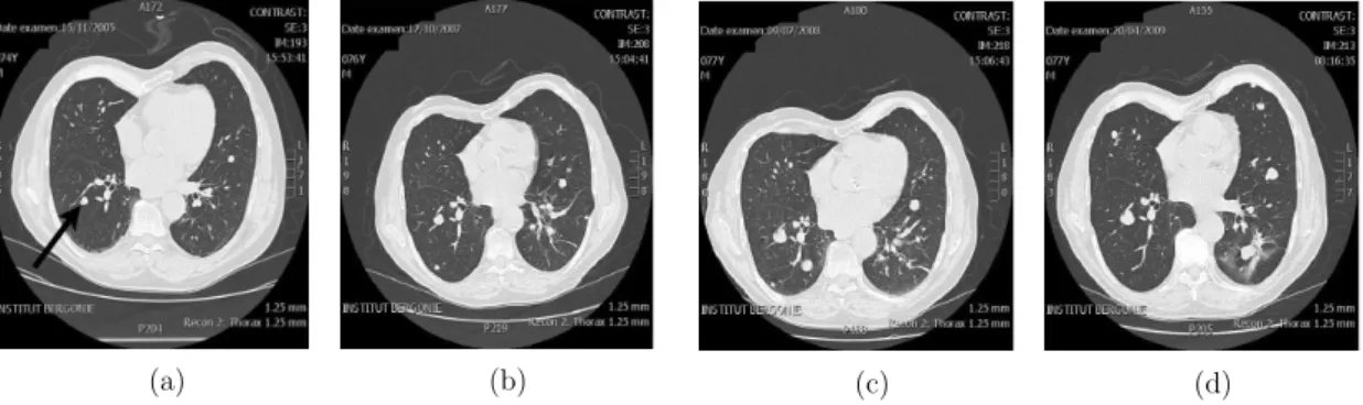
In Fig.2.2 four scans covering an evolution over 45 months are presented of some lung metastases of a primary tumor affecting the thyroid (Courtesy Institut Bergoni´e). Even though this patient is affected by several metastases, only the study of the one marked in Fig.2.2.a) will be presented. It is a quasi-steady metastasis, which grows very slowly and thus need only to be monitored. The results obtained by means of a sensitivity technique are presented, when only the first two scans were used in order to identify the system.

36 CHAPTER 2. INTRODUCTION

(c) (d)

Figure 2.2: Scans: a) November 2005, b) October 2007, c) July 2008, d) April 2009 This means that the first two images were used as data set to solve the inverse problem and find the set of control. Then, the direct simulation were performed covering the entire evolution and the result has been compared to the data of the subsequent exams.

The computational set up is detailed in the following chapters. In Fig.2.3 the volume of the scans is compared to the direct simulation. The solid line is the area of the simulated tumor (seen on a 2D slice), the black circles represent the area of the scans used as data and the red squares represent the predictions. This is a very promising result and it will be analyzed in detail. However this represents in some sort the best that may be achieved by a prognosis tool driven by medical imagery. In Fig.2.4 the fourth scan and the corresponding image are compared, showing a good agreement.

The first works considering realistic applications for tumor growth were based on ordinary differential equations. The presented results highlights one of the advantage of using models based on partial differential equations with respect to models based on ordinary differential equations. The latter, albeit simple and cheap from a computational standpoint, are not able to exploit all the available informations concerning the pathology, thus providing a less rich description of the phenomenon.

When targeting realistic applications several fundamental practical problems have to be tackled in order to set up a reliable tool. In particular, as it will be clear later on, images have to be preprocessed to be suitable for inverse problems. The first issue is segmentation: tumor and the surroundings have to be distinguished as well as the organ boundaries. This task may be very difficult in the case in which a tumor boundary is hardly defined and phenotypes are very diffused. Moreover, organs are often very deformable, which means that several external factors may influence what is observed on

Figure 1.1: Sequences of images, testcase presented in Section 1.1.

2.3. PARADIGMATIC RESULTS OF CLINICAL APPLICATIONS

37

0 5 10 15 20 25 30 35 40 45 50 4 5 6 7 8 9 10 11 12 13x 10 −3 months Area

Figure 2.3: Area as function of time for the slow rate growth. Solid line represents the

simulation results, black circles are the data used for the identification, red squares the

predictions.

(a)

(b)

Figure 2.4: a) Fourth scan b) Simulation

Figure 1.2: Evolution of a lung nodule, with slow dynamics, over 45 months. Test case presented in Section 1.1

possible to perform a forecast on the solid tumour evolution. The assumptions and the methods investigated are reported in details in [22]. We describe, here, a realistic testcase.

The (slow) evolution of a lung nodule (secondary tumour) is shown in Figure 1.1. A set of images on 45 months is available. The experiment consists in using the two first images of the sequence to performe the parameter estimation and use the rest of the sequence as a validation set. Using two images means restring to the least possible amount of information available.

In Figure 1.1, the result is shown in terms of area (in the image plane) as function of time. In the case of slow tumour growth, using two images can be enough to have a reasonable forecast. However, as observed in [22], there are cases in which more information is needed. In general, several methodological questions arise, namely about the parameters identifiability, the uncertainties a↵ecting the system, the reliability of the forecast.

(20)

1.2 Problems in haemodynamics

Systemic circulation is a complex multi-physic, multiscale system and the cardiovascular haemo-dynamics can be described at di↵erent levels (a comprehensive presentation can be found in [FQV10]). In particular, a hierarchy of mathematical model is defined, that could be useful to address the description of the haemodynamics in di↵erent contexts.

1. Circuit analogy: these are systems of Ordinary Di↵erential Equations (0D models), well suited to describe the global behavior of flow and pressure, in multiple points of the systemic vascular network, as function of time: Q(t), P (t), where Q is the flow and P is the pressure. In these models the flow plays the role of the current and the pressure plays the role of the voltage.

2. Hyperbolic network : 1D space-time Partial Di↵erential Equations models, adapted to de-scribe pressure waves through a reduced fluid-structure interaction model. The unknowns are flow and pressure along the axial coordinate of the blood vessels Q(x, t), p(x, t). The resulting equations for a single blood vessel are an hyperbolic system in subcritical regime. The couplings between di↵erent vessels is performed by considering the equations of the characteristics, mass and momentum conservation.

3. 3D Fluid-Structure Interaction (FSI): 3D incompressible Navier-Stokes equations to de-scribe the blood flow, coupled with non-linear elasticity to dede-scribe the vessel wall dynam-ics. It is the most realistic description of the mechanical behaviour of the blood vessels. The classes of models presented above can be derived by the 3D models by making some simplifying assumptions.

The use of one class of model depends upon the questions under investigation. In this Sec-tions, some contributions are presented in which these three classes of models are used (often in combination) to describe di↵erent subsystems of the arterial circulation, and perform data assimilation.

1.2.1 A sequential approach for the systemic circulation

Due to its prohibitive computational cost, the 3D FSI description of the whole arterial network is, at present, out of reach. In some clinical applications, as, for instance, the continuous monitoring of hypertensive patients, it is important to estimate the mechanical state of the blood vessels (especially close to the heart), by exploiting non-invasive or micro-invasive measurements taken at the periphery of the vascular network. This inevitably involves the need to describe the whole circulation or, at least, a large portion of it. To this end, 0D and 1D model need to be used. In this work, we use the most simple model proposed in the literature: let, for each vessel, x be the axial coordinate, the unknowns are the cross sectional area of the blood vessels A(x, t) and

(21)

Peer Review Only

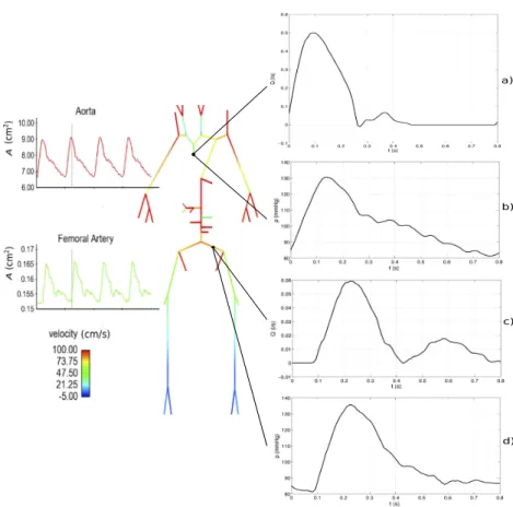
7 !" #" $" %"

Figure 2. Plot of the reference solution for the 55 main arteries of the human body. Solid colors are the mean velocity, between its minimum (blue) and maximum (red). Arteries cross sectional area vs. time is shown in two locations: the aorta inlet (red), the femoral artery (green). Moreover, flow rate

in l/s and pressure in mmHg are shown for the aorta inlet and the iliac artery.

the mean velocity of the blood flow (blue for the minimum and red for the maximum); the evolution in time of the arterial cross-sectional area is represented in the aorta inlet and in the femoral artery. On the left, four plots show the flow rate (in l/s) and the pressure (in mmHg) in the aorta inlet and in the iliac artery on one cardiac cycle, when simulation reached an almost periodic state. The solutions obtained are reasonably realistic in terms of shape and both pressure and flow rate have a correct order of magnitude.

Copyright c 0000 John Wiley & Sons, Ltd. Int. J. Numer. Meth. Biomed. Engng. (0000) Prepared using cnmauth.cls DOI: 10.1002/cnm

Page 7 of 29

http://mc.manuscriptcentral.com/cnm

International Journal for Numerical Methods in Biomedical Engineering

1 2 3 4 5 6 7 8 9 10 11 12 13 14 15 16 17 18 19 20 21 22 23 24 25 26 27 28 29 30 31 32 33 34 35 36 37 38 39 40 41 42 43 44 45 46 47 48 49 50 51 52 53 54 55 56 57 58 59 60

Figure 1.3: Example of a simulation of the 55 main arteries of the human body, Section 1.2.1.

ve average in the section blood velocity u(x, t). The resulting system of equations reads:

@tA + @x(Au) = 0, (1.8) @tu + @x ✓ u2 2 + p ⇢ ◆ = u A, (1.9) p = pe+ ⇣ A1/2 A1/2₀ ⌘. (1.10)

In this system pe represents the external pressure, A0 the cross-sectional area at rest, ⇢ =

1050kg/m3 _{is the blood density,  = 9}_{· 10} 6_m2_{/s accounts for momentum di↵usivity and} _is

related to vessels elasticity. All the details are commented in [23]. The discretisation of this model is perfomed by using a Taylor-Galerkin finite element method, with a number of degrees of freedom_{N ⇡ 8 · 10}3_{. At the bifurcations, mass and momentum continuity, and equations for the}

characteristics, provide the coupling conditions between adjacent vessels. The outlet boundary conditions are classical 3–elements Windkessel models. Overall, the model has approximately 130 free parameters. In Figure 1.3, an example of a simulation is provided, of the 55 arteries of the human body.

The available data are typically time sampled flow and pressure signals, taken in several peripheral points of the network. The nature of the data and the need to provide a fast estimation

(22)

motivated us to study sequential data assimilation methods. The contribution is threefold: 1. An Unscented Kalman filter is set up and applied to the 1D model of the 55 main arteries

of the human body.

2. Several semi-realistic test cases are proposed, in which the sti↵ness of the di↵erent segments of the aorta is estimated.

3. The sensitivity of the estimation with respect to the parametric uncertainty is studied. The scenarios considered are semi-realistic, data used are both synthetic and experimental (Only few experimental signals are available). The specific settings are provided in [23]. The method used to perform data assimilation is one of the non-linear extensions of the Kalman filter, the UKF.

One of the outcomes of the proposed model is to assess the precision of the techniques which are currently used to estimate the sti↵ness of the blood vessels. These are currently based, in the clinical practice, on the Pulse Wave Velocity (PWV), which is a measure of the average speed of the pressure waves in the vascular network. In particular, a standard test consists in recording the pressure signals in points of the femoral and carotid arteries, and estimate an average speed by evaluating the wave shift. This is one of the criteria used to assess the severity of the hypertension in patients. The estimations performed by using the 1D model are more precise if compared to the estimations obtained by measuring the Pulse Wave Velocity and computing the sti↵ness by means of the Moens-Korteweg formula (which relies on too restrictive geometric assumptions). Furthermore, one of the experimental observations is that, in a same patient, there are significant oscillation of the measured value of PWV during the day. The model used provides some insight and an interpretation of these oscillations in relation to the daily routine.

The use of 1D model could henceforth improve the sti↵ness estimation with respect to the currently used technique. However, after evaluating the sensitivity to random perturbations, the conclusion of this study is that, in general, a small number of measurements at the periphery, even if quite well resolved in time, are not enough to estimate the aorta sti↵ness in a robust way.

If the measurements available are rich enough (a concept to be well defined and quantified), for example by fusing multiple sources of information together, sequential approaches seem to be well suited to the estimation of hidden quantities in a time compatible with the clinical practice. The main difficulty to be circumvented is, therefore, to understand how many measurements and where they should be taken in order to reliably estimate the QoI. A step towards this direction is proposed in Section 3.1.

1.2.2 Retinal haemodynamics

Retina is part of the central nervous system, and an exceptional window on the micro-circulation: it can be easily imaged by standard optical techniques, such as fundus cameras. In [1], a model describing the mechanical behaviour of large arterioles (diameter d > 40 µm) is proposed. The fluid-structure interaction model used for this study is presented in Section 2.1.1 and in [2]. The main features of the model of retinal circulation are the following:

(23)

(a) (b)

Figure 1.4: Geometry of large arterioles, for the simulations discussed in Section 1.2.2: a) global view of the mesh; b) map of the control points for the comparison with the experiment detailed in [RRG+_86].

1. A 3D simplified fluid-structure interaction is built on a realistic geometry segmented by fundus camera.

2. A feedback control is added aiming at modeling autoregulation.

3. The actuation of the control is rendered through the addition of a model of Smooth Muscle Cells.

The geometry of the retinal network used is presented in Figure 1.2.2.a), and it is obtained by segmenting a retinal image acquired by means of a standard 40 Field Of View fundus camera. In Figure 1.2.2.a) the points in which the velocity (and the flow) are monitored is shown. The direct numerical simulations are obtained by discretising the model presented in in [1] by means of P1-P1 SUPG stabilised finite elements. The number of degrees of freedom is about 6_{· 10}5_.

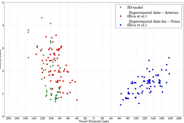
The parameters of the model are discussed in [1] and they are tuned in order to be representative of a physiological range. In this first work, the experiment presented in [RRG+86] is used as a validation. In their work, the authors studied experimentally the distribution in the network of the flow as a function of the diameter of the arterioles.

This comparison to real data is a first form of weak validation for the models used and show how data assimilation can be a valuable tool for mathematical modeling. The main sources of error, commented in [1], are due to the optical distortion in the periphery of the field of view (leading to an overestimation of the vessel diameters for the distal portion of the network) and on the fact that, when the diameter is small (normally d. 40 µm), non-Newtonian e↵ects could start playing a role in the blood dynamics.

(24)

Figure 1.5: Comparison to the experimental data, Section 1.2.2: the green markers represent the values extracted in the control points for the 3D model, to be compared to the red markers obtained experimentally.

(25)

This model has been recently adapted in an ongoing work, to provide a mathematical and physical interpretation of some hypotheses on the occurrence of micro-hemorrhages in the vas-cular network of the central nervous system.

1.2.3 State estimation from ultrasound measurements

Doppler ultrasound imaging is one of the most commonly used techniques to measure the blood velocity in a non-invasive way.

The reconstruct of a 3D blood velocity field on a human carotid artery from Doppler ultra-sound images is proposed. The images are synthetically generated (even if based on a realistic geometry) and the use of data from real patients is deferred to a future work. The main goal of the contribution is twofold:

1. A reduced-order optimal reconstruction method is introduced, that can be seen as a non-linear extension to the Parametrised Background Data Weak (PBDW) method. The main novelty is a partition of the solution setM = [K

k=1M(k)which we exploit to build reduced

spaces Vn(k) for each M(k).

2. Second, a non trivial application is proposed, the reconstruction performance between the classical PBDW and its non-linear extensions are proposed. These are the first step towards realistic applications

At every time t_{2 [0, T ], we are given a Doppler ultrasound image that contains information} on the blood velocity on a subdomain of the carotid. From the image, we extract the observations `i(u) that we will use to build a complete time-dependent 3D reconstruction of the blood velocity

in the whole carotid ⌦.

Depending on the technology of the ultrasound device, there are two di↵erent types of velocity images. In most cases, ultrasound machines give a scalar mapping which is the projection of the velocity along the direction n of the ultrasound probe. This mapping is called color flow image (CFI). In more modern devices, it is possible to get a 2D vector flow image corresponding to the projection of the velocity into the plane. This mapping is called vector flow image (VFI).

In the following, we work with an idealized version of CFI images. For each time t, a given image is a local average in space of the velocity projected into the direction in which the ultrasound probe is steered. More specifically, we consider a partition of ⌦ = _[m_i=1⌦i into m

disjoint subdomains (voxels) ⌦i. Then, from each CFI image we collect

`i(u) =

Z

⌦i

u· n d⌦i, 1 i  m, (1.11)

where n is a unitary vector giving the direction of the ultrasound beam. From (1.11), it follows that the Riesz representers of the `i in V are simply

!i = in,

where i denotes the characteristic function of the set ⌦i. Thus the measurement space is

Wm= Wm(CF I) = span{!i}m_i=1.

(26)

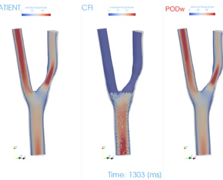
Figure 1.6: Result for the experiment commented in Section 1.2.3: velocity magnitude for the target solution (left), the CFI data (center), reconstruction (right)

Since the voxels ⌦i are disjoint from each other, the functions {!i}mi=1 are orthogonal and

therefore having a CFI image is equivalent to having

! =PWmu = m X i=1 h!i, ui!i= m X i=1 `i(u)!i. (1.12)

The PBDW method consists in a regularised least square method that manage to perform a trade o↵ between the model solutions and the data (both a priori and a posteriori knowledge are a↵ected by some errors). In its first version (noiseless measurements) it can be cast as an optimisation problem: u⇤ = arg inf u|h!i,ui=`i,8i kP?Vnuk 2 V, (1.13)

where_{V is the Hilbert space the solution u belongs to.}

The model used is the system of incompressible Navier-Stokes equations, in which the bound-ary conditions are imposed by using classical three elements Windkessel models. The details about the formulation are proposed in [15]. The solution set to be used is built by making the parameters vary in a physiological range. The solution set is partitioned based upon two pa-rameters that can be easily assessed in the online phase (the cardiac rhythm and the normalised time in the cardiac cycle). The optimal partitioning of the solution set is a problem which is far from trivial. In the present work, a partitioning based on the empirical evaluation of the reconstruction performances on the database is proposed.

(27)

1.6 the data (center) are acquired only in the first portion of the carotid artery. The paramet-ric Windkessel governing the outflow boundary conditions are used to mimic arterial blockage situations (that would correspond to an altered flow split with respect to the non-pathological configuration). The goal is to be able to predict these situations by using only the measurements in the first half of the geometry. The result shown in Figure 1.6 is a preliminary result in a semi-realistic setting. In particular, the reconstruction of the velocity field is quite accurate (er-rors are of the order of 1% in L2 _{norm), which is promising in view of improving and deploying}

the proposed strategy in more realistic settings. More details about the results of the numerical experiments are proposed in [15].

1.3 Data assimilation in cardiac electrophysiology.

Cardiac toxicity is part of the Safety Pharmacology, and consists in studying the negative e↵ects of drugs and chemical compounds on the cardiac function. The Comprehensive in vitro Proar-rhythmia Assay (CiPA) is an initiative for a new paradigm in safety pharmacology to redefine the non-clinical evaluation of Torsade de Pointes (TdP) [CVJS16, MDS+18, YKI+18].

A way of measuring the impact of a molecule of a given ionic channel is to consider the Patch Clamp, that consists in putting micro-electrodes across the cellular membrane and measuring the activity of the single cells (The transmembrane potential recorded as a function of time is called Action Potential, AP). This method is precise but low-throughput and hence time consuming. The need to have a high-throughput screening of molecules candidate to become a drug motivated the development of protocols to exploit devices such as the Micro-Electrodes Array (MEA). In this device, a layer of cells (cardio-myocites) is put into a well, in close contact to electrodes, that record the electrical activity. The observation of the electro-graph (the signal is called Field Potential, FP in what follows) conveys an information on the overall electrical activity and how it is eventually altered by a certain molecule. In the following, two cases are presented, with realistic data sets: in the first one, a stochastic inverse problem is solved, in which the probability density distribution of the model parameters is estimated in such a way that the statistics of the model outputs match the statistics on the experimental measurements; in the second one, a classification problem on MEA signals is described.

1.3.1 Stochastic inverse problems on action potentials.

The variability observed in action potential (AP) measurements is the consequence of many di↵erent sources of randomness. In this contribution we focus on parameter randomness which, in the context of AP modeling, corresponds to the natural variability of the cardiomyocyte electrical properties such as its capacitance, ionic channel conductances and gate time constants. Due to the large number of free parameters in AP models, these parameters are in practice unidentifiable [DL04], i.e. di↵erent combinations of these parameters can lead to the same AP. Therefore, we choose to restrict our analysis to a subset of ionic channel maximal current densities which are referred to as conductances in the following.

AP measurements may result from heterogeneity within a population of cells (inter-subject variability) [SBOW+14] or from dynamic variations within a single cell (intra-subject variabil-ity) [JCB+_{15, PDB}+_16].

(28)

Investigating the variability of AP models parameters has several motivations. For instance, it can be used to predict the response of cardiomyocytes to certain drugs [BBOVA+13], or it can provide insight into cell modifications at the origin of common heart diseases such as atrial fibrillation [WHC+_{04, SBOW}+_{14] or ventricular arrythmia [GBRQ14].}

There are two main strategies to estimate the parameters variability given a set of AP measurements. First, one could fit the AP model to each measurement individually and therefore obtain a set of parameters from which useful statistics may be computed. The problem of fitting an individual AP has been addressed many times and using a large variety of methods [DL04, SVNL05, LFNR16]. However, the computational cost of such a strategy may be prohibitive, especially for large datasets.

The second strategy belongs to the so-called population of models approach. The experimen-tal set is considered as a whole and the parameters statistics are estimated by solving a statistical inverse problem. Several techniques were developed to solve such problems [Kou09, GLV14] and their application to electrophysiology has recently generated much interest [MT11, BBOVA+13, SBOW+14, DCP+16]. The method developed in this contribution (called Observable Moment Matching, OMM) aims at estimating the parameters (thought as random variables) PDF in such a way that the model outcome statistics match the observed ones. The method is explained in detail in Section 3.2 and detailed in [19]. The OMM method is applied to the estimation of the PDF of key conductances from AP measurements. Several experiments are proposed in [29]. We report, hereafter, the results on experimental signals collected from human atrial cells.

The data consist in a set of published AP biomarkers recordings that are readily available online2_{. The AP are recorded from human atrial cardiomyocytes coming from di↵erent}

sub-jects [SBOW+14] . The data set is divided into two groups: one counting 254 Sinus Rythm (SR) patients and another one counting 215 chronic Atrial Fibrillation (AF) patients. Both groups exhibit a strong inter-subject variability in addition to the inter-group variability. The available biomarkers are: APD90, APD50, APD20, APA, RMP, dV/dtmax, V20. The ionic

model used is the Courtemanche-Ramirez model, in which 11 conductances were parametrised. All the details are available in [29].

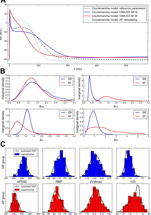
The results of the estimation of the PDFs of the parameters are shown in Figure 1.7. To each group is associated a most representative individual whose biomarkers values are the closest to the median ones of its group. The calibration step is very informative as it allows for a first comparison between the two groups, or more precisely between the two representatives of each group. The calibration leads to high di↵erences for gK1(+220%), gto(-100%), gCaL (-63%)

and gKur (-60%) which are qualitatively similar to those reported in [SBOW+14].

Beyond these inter-group variations captured in the calibration step, the inter-group vari-ability is revealed by the study of the estimated PDFs (see Figure 1.7 B). The results highlight the distribution di↵erences of gto and gKr between the two groups: in the SR group, these two

conductances feature a normal-like distribution whereas in the AF group those distributions are skewed and with a larger variance. The distribution of gN a are similar between the two groups

which suggests that it does not play an important role in the AF mechanisms. gK1also features

a much higher mean value and higher variance in the AF group. A posteriori distributions of the biomarkers of interest may be computed from the estimated PDF. When compared to the actual

(29)

! "!! #!! $!! %!! & '()* +%! +$! +#! +"! ! "! #! ,-'(.* /012&3(45673 (0839: 23;323563 <424(3&32) /012&3(45673 (0839: /=,>? ! ;"& /012&3(45673 (0839: /=,>? ,# ;"& /012&3(45673 (0839: ,# 23(0839"5$

!%! !%& '%! '%& "%! "%& (%! (%&

$)4 !%! !%' !%" !%( !%# !%& !%$ !%* !%% !%+ (42$"549 835)"&, ! ,#

!%! !%& '%! '%& "%! "%& (%! (%& #%!

$-' ! ' " ( # & (42$"549 835)"&, ! ,#

!%! !%& '%! '%& "%! "%& (%! (%& #%!

$&0 !%! !%& '%! '%& "%! (42$"549 835)"&, ! ,# ! ' " ( # & $ $-2 !%! !%" !%# !%$ !%% '%! '%" (42$"549 835)"&, ! ,# '!! "!! (!! #!! &!! ,-.+! ! $201< 3)&"(4&38 -.# 3/<32"(35&49

++! +%& +%! +*& +*! +$& +$!

!=-'! ''! "'! ('! #'! 8.8&(4/ +#! +"* +'# +' '" "& ."! '!! "!! (!! #!! &!! ,# $201< 3)&"(4&38 -.# 3/<32"(35&49

++! +%& +%! +*& +*! +$& +$! '! ''! "'! ('! #'! +#! +"* +'# +' '" "&

!

"

#

Figure 1.7: (A) CMA-ES parameter calibration of the Courtemanche model prior to the inverse procedure. APs obtained for the most representative samples of the SR (blue) and AF (red) groups, reference parameters (dashed) and after AF remodeling (dotted). (B) Courtemanche conductances estimated marginal densities for the SR (blue) and AF (red) groups. Conductances are normalized by the literature values. (C) Normalized histograms of the four experimental biomarkers of interest for both SR (blue) and AF (red) groups. The black solid lines correspond to the PDF of each biomarker estimated by OMM.

(30)

distributions (approximated by histograms of the experimental biomarkers), it shows that the OMM method succeeded in matching the variability in the measurements.

A point to be discussed is the use of biomarkers versus time traces. This is often imposed by the type of experimental data available. Ranges of biomarkers using standard protocols are easily accessed by experimentalists, and raw action potential data are not always available. It is therefore important to evaluate the use of both biomarker ranges and action potential traces. The set of available biomarkers is often dictated by experimental constraints. It is however possible, when there are many available biomarkers, to conduct a preliminary study to determine which biomarkers should be taken into account in order to recover certain parameters of interest. This issue is discussed in Section 3.3.

1.3.2 Classifying the electrical activity based on MEA signals.

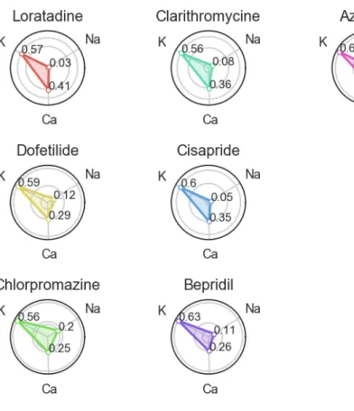
In this Section we describe how to classify the action of 12 compounds on the ionic channel activity based on in vitro data derived from Micro Electrodes Array (MEA) recordings of spon-taneous beating hiPSC-CMs (PluricyteR _{Cardiomyocytes) cultured on 96 well MEA plates (8} electrodes per well, Axion Biosystems), as described in [28].

The contribution of this work is twofold:

1. The in vitro dataset is complemented by an in silico dataset, obtained by simulating the experimental device in a number of meaningful scenarios.

2. The classifier used to produce the result is optimised to deliver optimal classification performances.

In vitro data used for this part are FP traces recorded from a hiPSC-CM monolayer (PluricyteR Cardiomyocytes, Ncardia) plated on a 96 well MEA plate (8 electrodes per well) Axion Biosys-tems3.

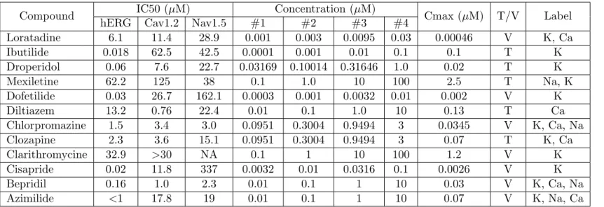
The 12 CiPA compounds listed in Table 1.1 were tested on PluricyteR _{Cardiomyocytes} and FP traces were recorded before and 30 minutes post compound addition. MEA results of 5 compounds were used for the training and MEA results of 7 ”blind” compounds for the validation.

Each compound was tested at 4 concentrations, 1 concentration per well and in 5 replicates (n = 5 per concentration). For this study only FP traces were recorded and used for the training and classification, no calcium transient measurements were performed. The final experimental sample size was 75 for the training set and 85 for the validation set (some wells were removed from the analysis due to quiescence or noisy signal observations).

To perform this application, several observations are crucial:

1. The number of available signals is limited; moreover, they do not cover the spectrum of potentially meaningful scenarios.

2. Several variability sources a↵ect the observable: one is related to the di↵erent behaviour of the ionic channels; the other is related to the experimental conditions, such as fluctuations in the temperature, heterogeneity of the medium, variability in the physical parameters. 3_{Axion Biosystems device: Classic MEA 96 M768-KAP-96}