The design, fabrication, and testing of a wind tunnel for the study of the turbulent transport of aerosols

THE DESIGN, FABRICATION, AND

TESTING OF A WIND TUNNEL FOR THE STUDY OF

THE TURBULENT TRANSPORT OF AEROSOLS

by

MALCOLM S. CHILD

SUBMITTED TO THE DEPARTMENT OF

MECHANICAL ENGINEERING IN PARTIAL FULFILLMENT OF THE

REQUIREMENTS FOR THE DEGREE OF

BACHELOR OF SCIENCE

at the

MASSACHUSETI'TS INSTITUTE OF TECHNOLOGY February 1992 Massachusetts All Institute of Technology Rights Reserved Signature of Author Certified by

---

...

--

--

·

flna',wtm n n rif A ~n I ; ii ai 1 T w~ ni rA~.1rg

25

©

THE DESIGN, FABRICATION, AND

TESTING OF A WIND TUNNEL FOR THE STUDY OF THE TURBULENT TRANSPORT OF AEROSOLS

by

MALCOLM S. CHILD

Submitted to the Department of Mechanical Engineering on February 17, 1992 in partial fulfillment of the requirements for the Degree of

Bachelor of Science in Mechanical Engineering

Abstract

An open circuit, induction wind tunnel was designed and constructed for use in studying the turbulent transport of aerosols. The tunnel was fourteen feet in overall length, with a test section measuring 43 inches (1.1 m) in length and with a 81 in2 _{(0.05 m2) flow area. For}

the particular application of this tunnel the flow within the test section was specified to have a uniform velocity over 95% of the test section width, background turbulence levels of less than 0.25%, and a velocity range of 0.5 to 10 m/s. It was also required that a means for creating isotropic turbulence of approximately 5% intensity be provided.

The aerosol, composed of micron sized water droplets, was injected into the inlet of the tunnel with compressed air atomizers. This produced aerosol concentrations of 238 particles/cc ± 50 at a speed of 10 m/s.

Testing of the tunnel shows that the flow within the test section is uniform over 93% ± 3% of the section inlet at a speed of 15.5 m/s, and that turbulence levels are approximately 0.2% ± 0.2% at x/M of 15 and a speed of 13.2 m/s. When a uniform grid of 1/8 inch rod, 5/8" mesh and a solidity of 36% is placed at the test section inlet, a decaying, turbulent flow field is generated. The mean turbulence level of this manipulated flow is 5.5%, ± 0.4 at x/M of 15 and 10.4

m/s.

There were two problems associated with the operation of the tunnel. These are the appearance of a small vertical velocity

gradient across the test section, and the inability to inject the aerosol directly into the tunnel plenum owing to the turbulence generated

by the injectors. Recommendations for remediating these shortcomings are included.

Thesis Supervisor: Prof. John H. Lienhard V

Table of Contents

A bstrac t.... ... ... ii

Table of Contents ... iii

A cknow ledgem ents ... iv

1 Introduction ... ... 5

1.1 B ackground ... ... 5

1.2 Current Task ... ... 6

2 D esign Criteria ... ... 8

2.1 Test Section Flow Specifications... ... 2.2 H oneycom b...8..

2.3 Screens ... 10

2.4 C ontraction ... 1 1 2.5 Test Section ... 14

2.6 B low er and M otor Selection ... ... 15

2.7 D uct W ork ... 1 6 2.7.1 Seeding Section ... ... 16 2.7.2 Exhaust... 16 2.8 A erosol Injection ... 1 8 2.9 Turbulence G eneration ... ... 19 3 Construction... 2 0 3.1 Inlet... 2 2 3.1.1 Straw B undle ... ... 2 2 3.1.2 Screens ... 2 4 3.2 Seeding Section... ... 2 5 3.3 C ontraction ... 2 6 3.4 Test Section ... 2 9 3.5 Corner... 3.6 Adapter & Vibration Damper... 3 1 3.7 Blow er M ounts ... 3 2 4 Testing ... 3 3 4.1 Procedure...3 3 4.1.1 Pitot-Static Tube ... 3 3 4.1.2 H ot W ire... 3 4 4.1.3 PD PA ... 3 6 4.2 Results ... 4.2.1 V elocity Profiles ... 3 9 4.2.2 Turbulence Levels ... ... 4 0 4.2.3 A erosol Characteristics ... 4 6 5 D iscussion ... ... ... 5.1 G as Phase ... 5 0 5.2 A erosol ... 5 3 6 Conclusion... 5 4 R eferences ... 5 6

Acknowledgements

I would like to thank the members of this project for their

assistance, conseling, and support during the course of this project. To Kurt Roth, many thanks for your support and fluids expertise crucial to the successful completion of the tunnel. To Jorg6 Colmenar6s, for your assistance, and perserverance in seeing this project through to completion. And to Prof. John Lienhard, for your invaluable advice and financial support.

I would especially like to thank my wife, Taintor, for putting up with my frustrations, absence, and preoccupation with the project. Your love and support have been a rock in an otherwise chaotic period.

This project has been funded by the Electric Power Research Institute under contract number RP8000-41 and through a UROP grant from the TRW Corporation.

1 Introduction

1.1 Background

Research on the behavior of small particles in a turbulent gas phase has application to large scale processes such as precipitation, pollution control, aerosol deposition, and fuel sprays. Current

research in the Heat Transfer Laboratory is investigating the Eulerian motion of small aerosol particles in a turbulent gas phase. In

particular, it is desired that a theory for the velocity and spectral statistics of a turbulent aerosol may be developed. Depending upon the balance of inertial and viscous forces a particle will tend to follow the streamlines of a flow , in the case of a sub-inertial particle; or, for a large inertial particle, they will slip from a given streamline.as the viscous forces on the particle are no longer able to confine it to the curviliner path of the turbulent eddies. The goal of the current research project is to acquire direct observations of the

instantaneous particle velocity and diameter in well defined and understood gas phase turbulence.

Previous experiments in this laboratory have employed an axisymmetric air jet as the gas flow component of the experiment (see figure 1). The aerosol was generated by commercially available high pressure sprayer. The jet device provided a well defined flow field for the aerosol, something that spayers themselves do not. The jet provides a 100 mm dia tube to allow the particles ample time to

slow down to the local flow velocity. The flow passed through a 200 mm mixing section, then into a 350 mm long, 80 diffuser to a 280 mm settling section. From there the flow exited through a 60-1

contraction to initiate vortex shrinkage and dampen turbulence. While this apparatus did remedy the problem of inertially induced velocity shifts inherent in the spayers, it had several other

Rlnwarn

Honey(

80 mm

:=13mm

uldinge %omrairers

FIGURE 1: Aerosol Jet Employed in Previous

Experiments in the Heat Transfer Laboratory, MIT. (Redrawn from Simo, 1991, p. 59)

problems associated with its operation.(Simo, 1991. p.1_{9) One of the}

problems was that it provided an insufficient number of large inertia particles. As can be seen in the schematic of the jet, two large

drainage containers were required to catch the large quantity of particles impacting on the contraction. Another problem associated

with the operation of the jet was the evaporation of particles far downstream of the outlet.

1.2 Current Task

studies. As such, this tunnel must address the following design criteria. In the test section of the tunnel, the aerosol must be

travelling in a well understood gas phase flow. The flow in the test section should have a uniform velocity across its test section with very low, ambient turbulence levels. Turbulence required for observations of the aerosol should be created in a well defined, isotropic manner, through the use of a uniform grid across the test section.(Tan-Atichat et. al.1982, & Corrsin 1963). In addition, the tunnel flow should carry an aerosol that is as dense as can be

without significantly affecting the the behavior of the gas phase, no more than about 0.3% mass fraction of water. High particle densities are important in order that particle turbulence power spectra be reliably resolvable. The aerosol should also ideally have a flat

distribution of particle sizes. This will allow a wide spectrum of sub-inertial and sub-inertial particle behavior to be analyzed.

2 Design Criteria 2.1 Test Section Flow Specifications

The design requirements for the wind tunnel are dependent upon the required flow characteristics of the test section. For the application of turbulent transport of aerosols it is required that the test section achieve a flat velocity profile (> 90% uniform velocity across test section), turbulence levels of less than 0.25%, and a velocity range of 2 to 10 m/s. To meet these requirements the following specifications for the tunnel were compiled:

* The test section should have a 9" (0.23 m) square cross section with a longitudinal dimension of approximately

48" (1.2 m).

* The tunnel should be an induction (suction) type to

eliminate the turbulence generated by a fan placed in front of the test section in a pressurized tunnel

* A series of flow manipulators, consisting of a

honeycomb, and a series of graduated screens should be placed in front of the test section to reduce velocity

components perpendicular to the flowand decrease the scale of the turbulent structures entering the tunnel * A 20-1 contraction should be used to enhance the attenuation of turbulence achieved by the honeycomb and screens

* The fan should be an axial type with an external motor

and continuously variable speed control.

2.2 Honeycomb

The honeycomb is located at the entrance to the tunnel to immediately straighten the flow and reduce velocity components

perpendicular to the flow. Experiments by Loehrke (1972) have shown that honeycombs with an L/d ratio of 60, where L is the length of the passage and d is the effective diameter of the passage, are most effective at reducing turbulence (p. 29). With this

specification in mind several suppliers of aluminum honeycomb were investigated as sources. These investigations led to the conclusion that a less expensive approach was needed. The required 48" square piece of honeycomb would have cost some where between 800 and 1800 dollars. It was decided that the same flow manipulation affect could be achieved by fabricating a honeycomb from plastic drinking straws.

Loehrke (1972) includes straws in his investigations of passive turbulence manipulators and found them to be particularly effective in quenching incoming turbulence (p. 29). He also found that

placement of a screen directly downstream of the straws increased the effective turbulence reduction. Loehrke notes that virtually all the turbulence found downstream of the straws was due to the

generation of new turbulence by shear-layer instabilities of the flow exiting the straws. The longer the straws, the more developed the emerging flow and the wider the wall wakes (p.30). When a screen was placed at the exit plane of the straws, the decay rate of the generated turbulence was dramatically increased. Loehrke attributes this effect to the more dissipative, smaller scales, generated by the screen shear layers (p. 32).

With these results in mind a combination straw and screen manipulator was selected as the inlet flow manipulator. The straws

covering the ends. The straws selected for the bundle are standard polyethylene drinking straws. The straws are manufactured by Diamond Straw, Inc. by an extrusion process that results in a smooth, seamless straw. They are 5.75" in length and 5/32" in diameter. This gives an L/d ratio of 36.8. As a assist to the fabrication process, the 75,000 straws required were purchased unwrapped. The screens selected for enclosing the straws are 20 mesh/inch, stainless steel screens with a wire diameter of .009".

2.3 Screens

Immediately following the straw bundle is a series of screens whose purpose is to further reduce the scale of the flow exiting the straw bundle. There are two important factors that influence the performance of the screens. These are, the solidity of the screen (a),

which is the ratio of area covered by wire, to the total area of the screen, and the mesh size of the screen (M).

The solidity of the screen effects both the pressure drop across the screen and its effect on the turbulence reduction of the screen. Corrsin (1944) has noted a coalescing of jets issuing from screens of greater solidity than 0.42. This phenomenon has the effect of

creating persistent mean velocity variations and reducing the decay rates of any induced turbulence.(Tan-Atichat, 1982 p. 503)

Mesh size determines the scale of the turbulent structures that pass through the screens. The size of the flow structures will be on the same order as the mesh size of the screen. To further reduce the scale that is exiting the combined straw/screen bundle at the inlet, a smaller mesh size was selected. As a 20 mesh screen (a = 0.33) was

downstream of the combined manipulator. The 24 mesh screen had a wire diameter of 0.0075", giving a solidity for each of the two screens of 0.33.

2.4 Contraction

The contraction used in the tunnel is scaled from a similar tunnel now employed in the Acoustics and Vibration Laboratory at MIT (Hanson,1967). The AV tunnel has turbulence levels in its test section of approximately 0.1%, and uniform velocity over 87% of the height of the test section. These guidelines are in the same range as the specifications for the aerosol tunnel. A scaling factor (Sc) for the two tunnels was determined from the ratio of test section

dimensions, 9" for the aerosol tunnel, and 15" for the A/V lab tunnel. For the two tunnels,

Sc = 1.67.

By the dividing the characteristic measurements of the AV tunnel contraction by this factor, the corresponding dimensions of the

aerosol tunnel contraction were determined. For the aerosol tunnel the following dimensions were found:

* Inlet size Li = 40.2"

* Outlet size Lo = 9.0"

* Length L = 43".

The profile curve of the contraction was derived from a ninth order polynomial by setting the function and the first six derivatives equal to zero at the outlet, and the first two derivatives equal to zero at the inlet (Hanson, p..6). With these steps in mind and the

dimensions determined above the curve of the contraction may be determined.

y(x) =ao + a, x + a2 x2+ a3x3 + a4x 4 + a5 x 5 + a6 x6 + a7 x7 + a8 x8 + a9g x9

y 1'-6'(0) = 0 y', y"(L) = 0 y(O) = 0 y(L) = 15.6".

L = 43"

When this system is evaluated it is found that:

y(x) = x7(a7 + a8 x + a9 x2),

where a7 = 6.717 x10-11.in-6, a8 = 8.884 x10-12.in-7, and a9 = -2.119

x10-13_.in-8

The function (y(x)) derived gives the curved profile of the

contraction (Figure 2). At the intersection of two adjacent panels the line of intersection

would follow this curve when viewed in the planes of projection of the two panels. In order to obtain the curve of intersection as it would appear if one of the panels was flattened the function was operated on with the line integral:

S(x)=X

J0

10 20 30 40 50

Length [in.]

Figure 2: Contraction Profile Calculated from a 9th

Order Polynomial (Equation 1)

By plotting S(x) vs. y(x) the flattened curve of intersection was obtained. This curve was used to fabricate the panels of the contraction.

2.5 Test Section

* Transparent walls for operation of Phase Doppler

Particle Analyzer (PDPA);

* Walls must be flat and straight with a relative

roughness of less than 0.005;

* Walls of test section should diverge slightly to reduce the pressure gradient along the length of the section;

* There must be access for instrumentation that will not

adversely affect the flow i.e. no leaks, or protrusions that may introduce turbulence;

* The test section should be as long as possible given the

size constraints of the laboratory.

With these specifications in mind the test section was designed as follows. The material for its construction was chosen to be Lexan for its optical properties and the smoothness of its finish. The top and bottom panels were aligned approximately 20 out of parallel giving a slight divergence along the length of section. This gave the test section exit dimensions of 9" in width, by 10" in height. The inlet was specified to be 9" square.

2.6 Blower and Motor Selection

The blower selection was based on a pressure vs. flow rate chart estimated from the initial tunnel design. The plot was

calculated for test section velocities of up to 10 m/s through its nine inch square area. After examining commercially available blowers, a

12" diameter, Vaneaxial fan produced by Industrial Air, Inc. was selected. The pressure-flow data for the blower is in tabular form so a superimposed PQ curve can not be shown for comparison, but the blower is rated for 1300 CFM at a pressure drop of 0.75 inches of

water. At this operating point, the blower is turning 2000 RPM, consuming roughly 0.3 HP. The configuration of the blower is of an axial variety, with an external motor mount. The external motor allows the impeller shaft and bearings, to be isolated for the flow within a central nacelle. This is an important consideration owing to the high moisture content of the flow.

The motor was selected based on the requirements of the blower. A DC motor was chosen for this application for its superior variable speed performance with respect to a comparable AC motor. The motor selected is a Indiana General, permanent magnet DC

motor, developing 3/4 HP at 2500 RPM. To control the motor an open control from KB Electronics, Inc. was selected. This controller operated on 120 volts AC input and produced 90-130 VDC output. It provides for infinite speed control between a maximum and

minimum value adjustable with trim potentiometers.

2.7 Duct Work

The remaining sections of the tunnel, consist of the seeding section and the exhaust ducts. These sections are essentially open ended boxes for containing the flow. The principle design criteria for these sections was to maintain a low surface roughness on the

interior. To achieve this, these sections were all constructed with smooth, fiberglass panels, supported by plywood frames. The frames served two functions in that in addition to providing support for, and maintaining the squareness of the panels, they also served as flanges for attaching adjacent sections together.

The seeding section is the largest piece of ductwork required. It measures 22" in length and 40.2" square. Due to the large area of each side of the seeding section, in addition to the frames around each end, three longitudinal frames were used on each side to prevent the sides from bowing inward during operation of the

tunnel. The center most of the three frames on both side panels also served as mounting platforms for the aerosol injection nozzles.

2.7.2 Exhaust

The exhaust duct work, that is all sections between the test section and the blower, consist of a small diffuser, a 900 elbow, and a square to round cross section adapter. The cross-sectional area of the exhaust ducting was bounded by the area of the blower selected. It is desirable that the flow not pass through a contraction

downstream of the test section hence the exhaust ducting should have an equivalent, or smaller area than the blower. The blower selected for the tunnel has a 12" diameter flow passage. To remain within the requirement just noted yet retain the maximum area for the exhaust ducting to reduce the pressure drop, the duct work was chosen to have a cross section of 10" square.

The diffuser and elbow were designed as a single unit to

reduce the number of pieces required. The function of the diffuser is to reduce the velocity of the flow around the corner, there by

reducing the associated pressure drop. To achieve this without separation, the diffuser has walls diverging by approximately 60.

Over the 4.75" length of the diffuser this expands the channel width from 9" at the outlet of the test section to 10" in the remainder of the

exhaust ducting. There is no divergence in the top and bottom walls of the diffuser as the vertical dimension of the test section outlet is already the required 10". In addition, a section of honeycomb is placed at the entrance to the diffuser to reduce any effects that the

downstream sections may 1.2" have on the flow

A 7" in the test section. The 900 elbow is immediately downstream of the diffuser. The elbow turns the Figure 3: Turning Vanes Profile and Separation

flow so that it

(2 of 12 vanes shown)

may be exhausted out of the laboratory window, and it employs a set of turning vanes to accomplish this with a minimal pressure drop. The design specifications for the turning vanes were taken from

Pankhurst (p.92). He notes that for thin vanes the ratio of vane gap to chord length is on the order of 0.25. He also notes that the leading edge should have an angle of incidence of between 00 and 50. A good shape appears to be a 900 circular arc with tangential projections at each edge. The projections do not significantly affect efficiency and provide an aid for aligning the vanes (Pankhurst p. 93).

The vane profile selected is shown in Figure 3. The vanes have a radius of 2.5" and a chord length of 4.7". With this chord length, a separation distance of 1.2" was calculated from Pankhurst's criteria. To span the entire corner, twelve vanes, 12" in length would be required.

2.8 Aerosol Injection

The aerosol injectors used in this apparatus essentially the same compressed air, atomizers used in the previous apparatus employed in the laboratory (Simo, 1991). In both devices the sprayers used are a Sprayvector System produced by Vortec, Inc.. The sprayers are equipped with three heads that produce different

spray patterns. The head employed by John Simo was an

atomizing nozzle that produces a highly directional spray of particles up to 200 gm in diameter. This nozzle was chosen for his particular application due the confined space it was enclosed in. For the aerosol tunnel under development a different nozzle is employed. The

atomizing nozzle produces particle with a large initial velocity. When coupled with the relatively large size of the particle this can create a great deal of turbulence in the surrounding fluid. The sprayer head selected for this application is a humidifying model. It produces a highly dispersed, low velocity aerosol with a particle range of up to 80 gim. The sprayer consumes 0.1-0.25 gallons of water per minute, at a pressure of 20 psig. The water is dispersed with a jet of 80-110 psig air, which is blown across the water outlets. To achieve the large particles densities desired, two sprayers are employed.

The final design detail is a means for producing an isotropic, decaying turbulence field in the test section. This is accomplished by placing a uniform grid across the entrance to the test section. As with the selection of the screens, choice of mesh size and wire diameter is based on the scale of the turbulence to be manipulated, and the requirement that the grid have a solidity of less than 40%. The appropriate scale for the turbulence desired in the test section is

on the order of one centimeter. With this in mind the following specifications for the grid were determined. The grid is to be comprised two sets of parallel rods, the rods having 1/8" diameter and located on 5/8" centers. This prodices a grid with a solidity of

36%. The two sets of rods are to be mounted perpendicular to each

other within a frame having the same inner dimensions as the inlet to the test section. The grid will be secured between the mounting flanges of the contraction, and the test section with bolts passing through the flanges and the frame of the grid. This mounting arrangement allows the grid to be securely held in place, with the least chance of leakage around the frame, while still being

3 Construction

The product of the design process was a wind tunnel composed of seven major components. These components are illustrated in Figure 4 and consist of inlet flow manipulators including honeycomb and screens; an aerosol seeding section with two injection nozzles; a 20-1 contraction with inlet & outlet screens; a 43" long test section; a

900 elbow; a square-round section adapter; and a vaneaxial blower.

The majority of the tunnel was constructed from fiberglass panels, supported by wooden frames. Each section of the tunnel has a flange at each end to facilitate attachment to mating sections. The

contraction and test section are the two sections that are not

constructed with these materials. The contraction and test section are both fabricated with acrylic panels.

The fiberglass panels that comprised most of the duct work of the tunnel were required to have a roughness of approximately

0.005 mm. Several iterations of the process of laying up the panels were required before this degree of smoothness was achieved. In the first iteration the fiberglass was laid up on a flat table covered with a layer of tautly stretched plastic. This process resulted in an unacceptable finish as the plastic was marred by irremovable creases that could not be stretched out. In order to achieve the desired

surface quality a great deal of hand finishing would have been necessary.

The second iteration consisted of applying several layers of epoxy to a polystyrene sheet. Preparation of the epoxy covered

0 0 O00 >1) r- c -PC r-4 --) rI) m

II

>

necessary to make the sheet sufficiently smooth. After sanding, the finished surface was then waxed and the fiberglass and resin

applied. When the fiberglass panel was peeled from the sheet it was noted that the surface finish of the fiberglass panel was acceptable. However, when it was removed from the sheet the fiberglass

remained adhered to several small areas of the epoxy coating, which were torn from the polystyrene sheet. On close inspection it was noted that the epoxy and styrene had delaminated in numerous places and that considerable repair would be necessary. It was decided that this process was too time and labor intensive and that another approach was necessary.

The third, and final iteration, consisted of attaching a sheet of 28 guage aluminum to a plywood backing. The aluminum already possessed the required surface quality, and the plywood backing provided a rigid and flat support. By waxing the aluminum and laying the fiberglass and resin on this surface, all the fiberglass panels required for construction of the tunnel were prepared.in a

few days. The surface finish produced by this process was excellent, being at least equivalent to the surface roughness of commercial window glass.

3.1 Inlet

3.1.1 Straw Bundle

The drinking straws are held in place by a fiberglass and wood frame covered on each end by a 20 mesh screen (Figure 5). The straws are arranged in a hexagonal close packed orientation and held

3"xl

Pine Fr

Clamp

iesh ens

Figure 5: Corner Detail of Straw Bundle

Partially Exploded View

in place by the pressure exerted by the surrounding straws. With an intake size of 40.2 inches square, approximately 72,000 straws, 5.75"

length were required to complete the bundle. The straws were

packed in the frame by tearing the top off of each box of 500 straws, and arranging the boxes in rows within the frame. After laying a row of boxes, open end in, the boxes were slid off the straws and the entire frame was agitated to settle the straws. Using this method the entire straw bundle was packed in approximately 90 minutes. After, and during the packing process, the straws were carefully examined to eliminate warped, kinked, short or otherwise misshapen straws. The straws were packed into the frame until no settling was

packing the bundle until it was hung on the tunnel, some additional settling did occur. As a result, an additional 1000 straws had to be

dAA A aUUU LV 1 1 bundle before it was hung. _Clamp Screw: 3.1.2 Screens Fram ScreN The screens are 24 Mesh Screen I go i• I a ýii a l•

mounted in _{Figure 6: Corner Detail of a Typical}

wooden Screen Frame; Partially Exploded View

frames to

allow them to be removed or changed during the life of the tunnel. The frames were made from 3" x 1/2" clear pine straps and joined at the corners with half-lap joints, fastened with three 1/2" wood

screws in each joint (Figure 6). The corner joints provided good

strength and retained the thickness of the frames at the corners. The frames served a dual function as in addition to providing support for the screens, they also served as spacers to provide the necessary separation

distance between the screens. _{Great care was taken to ensure that} the screens were free from wrinkles or creases, and that they were mounted tautly within the frames. Each screen was sandwiched between a pair of frames which were then fastened by 1" wood screws. The mounting process was begun in the middle of one side

of the screen/frame sandwich and proceeded around the frame in both directions simultaneously. This ensured that the screens were evenly tensioned within the frames.

3.2 Seeding Section

The seeding section is the next section down stream of the flow manipulators. It is constructed of fiberglass panels supported by frames/flanges at each end and three longitudinal stringers on each side. The flanges at each end maintain the squareness of the section and allow for its attachment to the screens and straw bundle

upstream, and the contraction downstream. The longitudinal

stringers provide support for the sides of the section to prevent them from deflecting inwards due to the pressure differential created

when the tunnel is operating. The middle stringer on two opposing sides of the section are also used to support the aerosol injector. The injectors are placed near the leading edge of the seeding section and mounted in a curved slot cut into the center stringers. The curved

slots allow the angle of the sprayers to be adjusted from 900 to 450 with respect to the flow.

3.3 Contraction

Fabrication of the contraction was the single most laborious part of the construction process. This was due to need to join the compound curves of adjacent panels squarely and precisely. As

shown in Figure 7, the contraction is constructed from 1/8" Lexan with plywood and acrylic supports. Each side of the contraction was constructed separately, in the following manner. The curves

were transfered to a transparent sheet for use on an over head projector. The image was then projected onto the Lexan sheets, and after carefully measuring critical dimensions at the inlet, exit, and along the length, the image was traced on the Lexan sheet. Great care was taken in the measurements to ensure that the projection did not distort the shape of the curves. After tracing the curves on the Lexan, the actual contraction profile, not the line integral

projection, was traced onto sheets of 3/4" plywood. These plywood pieces would form the backbone of the supports for the Lexan sheets. The Lexan was cut to its rough shape with a saber saw then carefully ground to its final outline with a cylindrical sander. When the sides of the contraction were cut the top and bottom pieces were left with a two inch overhang along each edge to provide a surface for joining the sides together.

After forming the sides the next step in constructing the

contraction was to prepare the supports for each side. The supports for each side consist of a plywood backbone running the length of the contraction along the center line.

Pine Face

Frame

Figure 7: Assembled Contraction Looking Upstream Plywood and Acrylic Supports on Lexan Panels

Attached to the backbone are five one inch square acrylic rods evenly spaced along the length of the curve. The rods are recessed into the backbone to maintain the smoothness of the curve and are fastened to the plywood with 3" countersunk wood screws. Between each pair of rods are two one inch acrylic cubes bolted to the

backbone which provide additional attachment points between the support and panel. The sides of the contraction were attached to the acrylic supports with an acrylic adhesive and many clamps.

During the process of bending each side to its frame and supports a problem with our design was encountered. The leading edge of each side was located at the tangency point of the inlet curve. As a result there was not sufficient material to apply a couple at the leading edge to form the tight radius of the inlet curve. To form this part of the contraction it was necessary to use six jig/support blocks along the width of the edge. Each block was cut to the profile of the inlet curve and allowed the Lexan to be clamped and bonded to the proper shape.

After each side was bent to its final shape the four panels of the contraction were joined. To join the panels together a series of acrylic blocks were bonded along each edge of the two side panels. The blocks were then ground to the proper angle to permit the sides

and upper and lower panels to mate with no gap along the corner. The blocks were then clamped and bonded to the projecting flanges of the top and bottom panels. While joining the panels great care was taken to assure that each panel was mounted squarely to its neighbors.

3.4 Test Section

The test section is fabricated from 3/8" Lexan. The test section is essentially a 34" long box measuring nine inches square at the inlet and nine by ten inches at the outlet. The sides of the test section are bolted the top and bottom with 6-32 machine screws inserted into threaded holes along the edge of the top and bottom panels. Flanges at each end of the test section are made from one inch square acrylic rod bonded around the perimeter of each end.

There are two other features of the test section that are note worthy. Along the top of the test section a 1/4" slot is machined along the length of the test section to provide instrumentation access to the test section. The slot is sealed from leaks by two strips of

black rubber as shown in Figure 8. The rubber is recessed into the inner surface of the top and butted together along the center line of the 3/8" slot. This allows probes to be inserted into the test section with a minimal amount of leakage around to probe. In addition to the instrumentation slot, there is a five inch diameter access port cut into one side, near the outlet of the section. The port is closed with an acrylic plug, and sealed with an O-ring around the plug. This port

allows direct

6-32 Round Head

Machine Screw access to the

Intrumentation Slot

interior of the test section for cleaning the walls, and for insertion of instrumentation

ia~g~ g : Cross Sectional View of Upper that cannot be

Corner of Test Section, Showing

be passed Instrumentation Slot and Gasket

through the rubber gasket of the instrumentation slot (i.e. hot wire sensors).

3.5 Corner

Immediately downstream of the test section the flow is

duct with a set of turning vanes is employed. The corner, illustrated in Figure 9, is constructed of fiberglass panels with wood frames, and the turning vanes and fabricated from 28 guage aluminum. As with the other sections of the tunnel, the frames at the ends of the corner section act as mounting flanges for attaching the section to adjoining ones. At the inlet to the corner section there is a small diffuser that expands the flow passage from the 9 inch width, in the test section,

to the 10 inch square area of the exhaust ducting. The diffuser is very short (4.75 inches) and is immediately followed by the turning vanes. The :T VJFD turning vanes are constructed

FIGURE 9: 90* Elbow and Diffuser Section

from the same w/ One of Fourteen Turning Vanes Withdrawn

aluminum sheet that was used to lay up the fiberglass as described at the beginning of this chapter. The aluminum was cut to the proper

The vanes are fixed in the corner section by inserting them through curved slots cut in the top and bottom panels of the corner section. The slots were cut in both panels simultaneously to assure that the vanes would be square within the section. After insertion, the protruding ends of the turning vanes were cut in to a series of tabs which were bent over in alternating directions to secure the vanes. After bending the tabs over the area over the ends of the turning vanes was sealed with fiberglass and large amounts of resin.

3.6 Adapter & Vibration Damper

The final section of the tunnel before the blower is an adapter wherein the square cross section of the tunnel is gradually

transformed to a circular cross section for attachment to the blower. Connecting this section to the blower is a rubber collar that isolates the vibrations of the blower from the tunnel. The adapter section was formed from fiberglass on a polystyrene mold. The mold was constructed from twelve layers of one inch polystyrene, aligned axially on a piece of 1/2" pipe, and bonded together with an epoxy adhesive. The end layers of the mold were carefully cut to

correspond to the desired dimensions of the inlet and outlet. One end consisted of a twelve inch diameter circle while the other end was a ten inch square. The remaining ten layers of the mold were all made somewhat oversized to allow for fairing. After fairing the mold with a batten and a surfoam shaper, the mold was sealed with

several coats of epoxy and sanded smooth. Fiberglass and resin were then applied to the mold. When the resin had cured the mold was broken out from the fiberglass section and frames were attached to

The rubber coupling was attached to the adapter section and to the blower by bolting it to the flanges of both section. Lexan

clamping rings, made from left over pieces, were used over both ends to ensure that the rubber was evenly and securely fastened to the flanges.

3.7 Blower Mounts

The blower and motor assembly is mounted on a cradle made with angle iron supports and a plywood saddle. The cradle is

securely bolted to the cement window ledge. The blower exhausts the flow from the tunnel out of a window in the laboratory. This configuration required that one pane of the window be removed and replaced with a 3/4" plywood insert. This allows the blower to

exhaust out the window while keeping the window closed. The plywood insert is securely fastened to the window frame with aluminum clamps. One end of the blower is supported by the

plywood saddle of the cradle while the other is bolted to the plywood window insert. All the fastenings involved in the attachment of the

insert to the window frame, and the blower to the plywood insert, are configured such that they eliminate accessibility from the outside, keeping the window secure. The blower is attached to the plywood insert with carriage bolts, with the heads on the outside, and the aluminum clamps are screwed from the inside. The blower exhaust opening is covered by a gravity activated louvre that opens and closes automatically when the tunnel is started or stopped.

4 Testing

4.1 Procedure

Three testing procedures where used to characterize the flow in the test section of the wind tunnel. They were, a pitot static probe for velocity distribution and calibration measurements, a hot wire anemometer for turbulence measurements, and a Phase Doppler Particle Analyzer (PDPA) for measuring the characteristics of the aerosol. Pitot probe measurements where taken at four stations along the length of the tunnel, these being at four, fourteen, twenty four and thirty four inches from the inlet. Measurements with the hot-wire and the PDPA were taken at seven stations along the length of the test section. The placement of these stations was based on the mesh size of the turbulence generator placed at the entrance to the test section. The stations were positioned at intervals of 5 mesh lengths, and extend from 15 to 50 mesh lengths downstream. 4.1.1 Pitot-Static Tube

The pitot-static tube used was 1/8" in diameter and 12" long. It was equipped with a fiction nut that could be threaded into a support and that would grip the tube, fixing its position. By

loosening the nut a semi-turn the pitot probe could be moved to new position a fixed. The probe was mounted on a support that fit in the

top of the test section and could be placed at any position along its length. With these two fixtures a series of measurements where taken at the four stations along the test section.

At each station measurements were taken with a MKS differential pressure transducer, monitored with a MKS signal

conditioner. The transducer operated at a temperature of 400_{C and} was equipped with an internal heater. Power for the heater was supplied by the signal conditioner. Measurements at each station were made in Pascals at 0.25" increments, starting and finishing at 0.125" from each wall. These measurements provided vertical velocity profiles at each of the four stations in the test section

4.1.2 Hot Wire

Hot-wire measurements were taken at seven stations using an Intelligent Flow Analyzer (IFA-100) from TSI, Incorporated. The instrument consisted of a 5 tim, tungsten wire sensor, model T1.5, a probe support and 15' cable, and a central processing unit. Setup

and tuning of the hot-wire sensor was fairly straightforward, the processor doing most of the work. After mounting the probe support

on the test section a shorting wire was inserted into the support end to close the circuit, the processor was powered up and the display zeroed. The resistance of the cable and probe support were then measured, and entered into the IFA. After this initial setup, the wire sensor was inserted into the support readying the system for

frequency response tuning.

Frequency tuning was conducted with the tunnel operating in its highest speed setting. The bridge in the IFA was then set to the overheat-ratio recommended for the particular sensor employed. Tuning the probe consisted of generating a square wave test signal with the IFA and monitoring the response of the probe with an

oscilloscope. By adjusting the amplitude and frequency of of the test signal along with bridge, and cable compensation controls, the

response of the sensor was adjusted until it displayed a 13% overshoot to the step input.

After the sensor was tuned, it was calibrated with the pitot-static probe described above. The two probes were mounted in the same support with the hot-wire approximately one inch above the tip of the pitot tube. A series of measurements were taken at varying velocities. The values obtained from the two instruments (Pa from the pitot tube & Volts from the IFA) were then related through King's Law by:

E2= A + B U1/ 2 _[1]

where U is the velocity measured with the pitot tube, E is the voltage output from the IFA and A and B are the calibration constants. With these two constants the voltage values observed on the IFA could be reduced to velocities.

Measurements were taken at the centerline of the test section at the seven data stations. A series of measurements were taken at each station, over the full range of speeds sustainable in the tunnel, and, with and without the turbulence grid mounted on the test section. Mean velocity measurements were taken from the IFA and fluctuations due to turbulence were monitored with a Fluke model 8010A, digital multimeter configured to read true RMS voltage. Both of these values, mean and RMS voltages, were noted for each

combination of speed and station. The mean velocity values were converted using equation 1 above. The fluctuating velocity values taken from the multimeter were converted using the time derivative of equation 1. Differentiating equation 1, implicity, while holding the

2Ee' Bu'

2U1/2 _{, [2]}

where e' is the RMS voltage fluctuation measured with the

multimeter, u' is the RMS velocity fluctuation, and E, U, and B are the same as in equation 1. Solving for u' and substituting for U112 _gives:

u' = 4EU1/2 _{e' 4E(E} 2_{- A) e'}

B B2 . [3]

This is the relationship that was used to calculate the turbulence intensity of the flow. The turbulence intensity is the ratio of fluctuating velocity to mean velocity, specifically:

T.I. =UMS

U . [4]

As measurements with the hot-wire were made it became apparent that the signal produced by the turbulent fluctuations in the flow were of the same order of magnitude as the electronic noise inherent in the system. To reduce the amount of noise present, a low-pass, Butterworth type filter was employed. The filter was set to a cutoff frequency of 10 kHz. This reduced the amount of noise present in the signal by roughly 50%.

4.1.3 PDPA

The PDPA (Phase Doppler Particle Analyzer) was used to measure several characteristics of the aerosol seeded flow in the tunnel. For the purposes of this investigation, turbulence intensity, particle number density, and particle size distribution are the

characteristics of interest. The PDPA is manufactired by

Aerometrics, Inc., and operates on the principles of laser-doppler velocimetry (LDV). LDV employs the light scattered by a particle

passing through the intersection of a pair of converging laser beams. LDV is able to determine the velocity of a particle by measuring the doppler shift in the wavelength of the scattered light. The PDPA differs from standard LDV in that it is able to determine the size of the particle as well as the velocity. This is accomplished by using a series of detectors to measure the doppler burst produced when a particle passes through the probe volume, i.e. the volume of

intersection of the beams. Comparison of the phase shift detected at each of the sensors allows the diameter of the particle to be

determined.

The system used in the experiments is composed of two major components, optics and electronics. The optical units consist of a pair instruments mounted on either side of the test section on a bed

attached to a pair of rails that allow the optics to be placed at any position along the length of the test section. Vertical positioning was accomplished by adjusting the height of the table on which the rails are mounted. The table is equipped with a pneumatic cylinder that allows it to be raised or lowered. The optical units are both inclined,

150 toward the top of the tunnel to position the detectors at the

proper angle for receiving the doppler bursts. The emitter consists of a helium-neon laser, beam splitter and optics for focusing the beam pair. The detector is equipped with optics for focusing the burst onto the sensors. The supporting electronics include a motor controller, signal processor and a computer for data storage,

processing and operating the instrument.

manufacturer's specifications for the particular flow being examined. For example, the physical properties of the particles such as density, and index of refraction must be entered, and the proper optics for the size range expected must be selected. Once the system has been set up, operation consists of turning on the laser and electronics, and selecting velocity and diameter ranges to be measured. The optics are then positioned at the desired location and the measuring process initiated by pressing the appropriate key on the computer. The data acquired is displayed on the computer as histograms of the velocity and size distribution.

The display also includes information on number density,

velocity fluctuations, and the signal validation rate. The validity of a signal is determined by comparing the phase information of each of the series of sensors. If the phase information does not meet certain specifications then the signal is rejected. Some causes for rejection can be multiple particle in the probe volume, or over or under sized particles. The validation rate compares the number of acceptable

signals, to the total number of particles passing through the probe volume. The data display presents the number of measurement attempts, the validation rate, and number of rejected attempts. The rejected attempts are counted and displayed according to the criteria for their rejection. Each measurement run continues automatically until it is manually terminated or approximately 10,000 valid

readings have been acquired. The acquired data is then saved in the computer before the next run is taken. Software provided in the computer allows the data from many runs to be compared, averaged,

and presented in several different forms, permitting the most convenient or informative method to be employed.

4.2 Results

During the period over which the measurements were taken, it became apparent that there were irregularities in the performance of the tunnel. Initial tests with the aerosol injectors positioned in their slots in the seeding plenum, and without the turbulence grid in

position, indicated that the injectors were producing an unacceptably high level of turbulence (>5%). Also the screen placed between the injectors and the contraction quickly became blocked by water

impacted from the aerosol. As this situation was not acceptable, the following modifications were implemented. The screen between the seeding section and the contraction was removed, and the aerosol generators were moved from the seeding plenum to a position

directly in front of the straw bundle. While this change dramatically reduced the level of turbulence in the test section, it resulted in a large loss of particles as they became entrained in the straw bundle. Another consequence of the modifications was the presence of a vertical velocity gradient in the test section.

4.2.1 Velocity Profiles

The velocity profiles measured with the pitot probe are shown in Figures 10 through 13. These measurements were taken before

section and the contraction still in place. The measurements indicate that a uniform velocity of 93% ±3% is

obtained in the case the highest flow rate, at the station nearest the inlet. The uniform distribution decreases with distance from the inlet. It reaches its smallest level of 80% ±3% at 34 inches

downstream, at the highest flow rate.

Velocity profiles taken after modifying the configuration of the tunnel are shown in Figures 14 and 15. These profiles were taken with the hot-wire sensor in the same manner as the previous profiles. The configuration of the hot-wire probe did not allow measurements to be taken within an inch of the top of the test section. The plots compare the velocity profiles with the inlet

honeycomb approximately 60% clogged with water, with and without the turbulence grid in position, and after the honeycomb had been cleared with a blast of compressed air. This plot shows that the entrainment of water in the honeycomb had little, if any effect on the presence of the velocity gradient.

4.2.2 Turbulence Levels

Turbulence levels were measured along the center line of the test section with both the hot-wire and the PDPA. Figure 16 shows the turbulence levels measured without the turbulence grid in position. The measurements indicate that background turbulence levels, with a clear straw bundle are 0.2% ± 0.2% at x/M of 15 and a speed of 13.2 m/s. The reason for the high uncertainty in these measurements is that the turbulence signal from the hot-wire is of the same order of magnitude as the electronic noise inherent in the

set to a cutoff frequency of 10 kHz, the remaining noise was still of the same magnitude as the signal.

Flow Rate: 0.81 m^3/s; 93% Uniform +/-3%

Flow Rate: 0.44 mA3/s; 93% Uniform +/-3%

liml...-- A. 0 d0% .- Anl 1. n I . I nAl

0 a-0 o 0_ez oe 0 o U/Umax

Figure 10: Pitot Probe Velocity

(4" from inlet); Umax = 15.5 m/s;

Flow Rate: 0.81 m^3/s;

Flow Rate: 0.44 m^3/s;

Flow Rate: 0.12 mA3/s;

0.2 0.4 Profile at Height = 0.229 m 90% Uniform +/-3% 90% Uniform +/- 3% 90% Uniform +/-3%

0

Figure 11: Pitot Probe Velocity Profile at

1.0 0.2 0.4 0.6 0.8 1.0 0.6 0.4 0.2 0.0 -0.2 -0.4 .tfl A 0.0 0.0 1.2 Station 1 0.2 0.0 -0.2 -0.4 -0.6 0.0 1.2 YI _ _ _ · I · ·B -I - I -

-rI

i

Flow Rate: 0.81 mA3/s; 82% Uniform +/-3% Flow Rate: 0.44 mA3/s; 85% Uniform +/-3%

I•1... n-&-. ^ 4fl .A.J .. ^ - '-OI I I S. .--, .I 'J0!

0.2 0.4 0.6

Figure 12: Pitot Probe

Station 3 (24" from inlet); Umax =

Flow Rate: 0.81 m^3/s; 80% Flow Rate: 0.44 m^3/s; 86% Flow Rate: 0.12 m^3/s; 88% U/Umax Velocity Profile at 15.1 m/s; Height = Uniform +/-3% Uniform +/- 3% Uniform +/-3% S . I 1.0 1.2

Figure 13: Pitot Probe Velocity Profile at o 00 0 oe z o0 0 V C o C o ( 0.6 0.4 0.2 0.0 -0.2 -0.4

_n a

w/o Turbulence Grid: Cloaaed Straw Bundle Center Line 0.1 0.2 0.3 0.4 0.5 0.6 0.7 0.8 0.9 1.0 1.1 Figure 14: Station 0; U/Umax

Hot-Wire Velocity Comparison x/M = 15; Umax = 14.9 m/s

w/o Turbulence Grid; Clear Straw Bundle w/ Turbulence Grid; Clogged Straw Bundle w/o Turbulence Grid; Clogged Straw Bundle

A B A A A 0 A BA MA Center Line ₀ a M A * A * A BI ,.~~ []p~ &C8 0.1 0.2 0.3 0.4 0.5 0.6 0.7 0.8 0.9 1.0 1.1 Figure 15: U/Umax

Hot-Wire Velocity Comparison 0.8 0.6 0.4 1.U 0.8 0.4 0.2 0.0 ,i r F H I . |

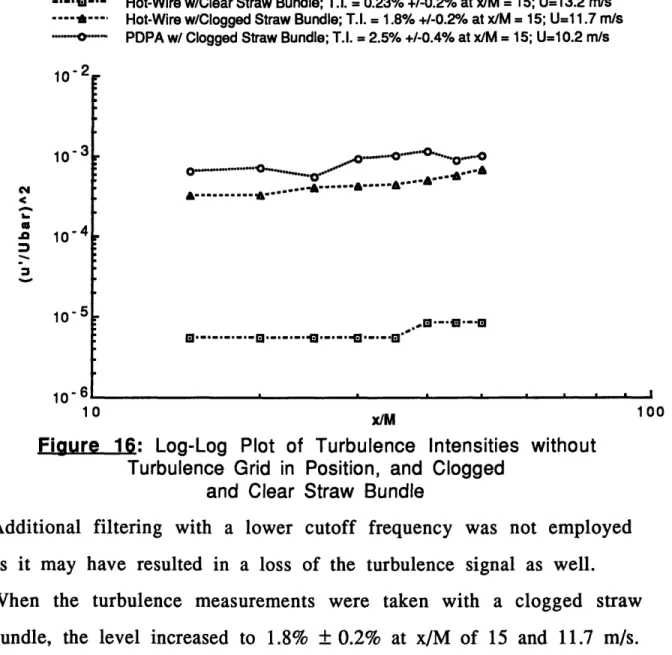
.-.***-- Hot-Wire w/Clear Straw Bundle; T.I. = 0.23% +/-0.2% at x/M = 15; U=13.2 m/s

----.a--- Hot-Wire w/Clogged Straw Bundle; T.I. = 1.8% +1-0.2% at x/M = 15; U=11.7 m/s

.---.-- . PDPA w/ Clogged Straw Bundle; T.I. = 2.5% +/-0.4% at x/M = 15; U=10.2 m/s

-2' 10-3 N a 10- 4 10-5 in- 6, ... ... ...--r [] ††††††††††††††††††††††††††††††††-I I I I I ' " • 10 x/M 100

Figure 16: Log-Log Plot of Turbulence Intensities without Turbulence Grid in Position, and Clogged

and Clear Straw Bundle

Additional filtering with a lower cutoff frequency was not employed as it may have resulted in a loss of the turbulence signal as well. When the turbulence measurements were taken with a clogged straw bundle, the level increased to 1.8% ± 0.2% at x/M of 15 and 11.7 m/s. The PDPA showed an a turbulence level of 2.5% ± 0.4% at x/M of 15 and 10.2 m/s.

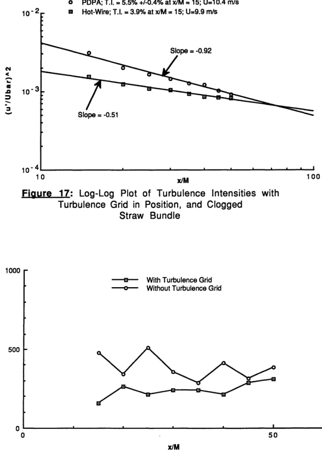
Figure 17 shows the turbulence measurements in the presence of the turbulence grid. As with the measurements shown in Figure 16, the turbulence levels measured with the hot-wire are slightly less than those measured with the PDPA. The levels recorded are 3.9% ± 0.2% at x/M of 15 and 9.9 m/s, for the hot-wire, and 5.5% + 0.4% at x/M of 15 and 10.4 m/s, for the PDPA. The maximum

disagreement between the two instruments is 1.6% at x/M of 15, and the minimum is 0.3% at x/M of 50.

4.2.3 Aerosol Characteristics

PDPA measurements of the aerosol number density are displayed in Figure 18. The point represent an average of many individual sampling runs at each station. In the case with the turbulence grid, 20 runs at each station are averaged. In the case without the turbulence grid, 10 runs are averaged.

Figure 19 shows the particle size distribution as the probability that a particle will be of a given diameter. Distributions are given for each of the seven stations. For comparison, Figure 20 is the same plot made for the jet apparatus, previously employed by John Simo (1991).

o PDPA; T.I. = 5.5% +/-0.4% at x/M = 15; U=10.4 m/s 10" L1

S10--=

Figure 17: Log-Log Plot of Turbulence Intensities with

Turbulence Grid in Position, and Clogged Straw Bundle

--- With Turbulence Grid

-0 Without Turbulence Grid

x/M

Figure 18: Aerosol Number Density vs. Distance Donwstream,

100

1000

1.6 1.2 Co .8 0 0 5 10 15 20 Particle diameter dp (jlm)

Fihure 19: Particle Size Probability Distribution for Tunnel

Each Line Representing One of Seven Stations

.3

0

.1

2 6 10

Particle Diameter (jxm)

Figure 20: Particle Size Probability Distribution for Jet Apparatus (from Simo, 1991. p. 138)

5.1 Gas Phase

The velocity profiles taken with the pitot probe, Figures 10 through 13, indicate that the original configuration of the tunnel produced the desired uniform velocity profile in the test section. They show that the contraction is performing as it should, and that the scaling of the contraction employed in the Acoustics and

Vibration Laboratory tunnel was an appropriate means for

generating the contraction profile. The development of the velocity gradient shown in Figures 14 and 15 is puzzling.

Hypotheses to explain the appearance of the gradient include, removal of the screen immediately proceeding the contraction, entrainment of water in the straw bundle at the inlet to the tunnel, and misalignment of the contraction and test section. Tests were performed to confirm or reject these hypotheses. Testing the effect of the screen on the flow in the test section was performed

indirectly. Due to the need to make many measurement of the behavior of the aerosol during the testing period it was not

convenient to replace the screen to its original position. With the aerosol generators placed outside the inlet of the tunnel a majority of the particles were being lost in the straw bundle. Replacement of the screen would have increased this loss, further reducing the

robustness of the aerosol. For this reason the screen was not replaced. However, the effect on the flow produced by the screen can be somewhat mimicked by the effect of the turbulence grid placed at the entrance to the test section. The pressure drop

than that of the screen. If the loss of pressure drop associated with the removal of the screen was the cause of the velocity gradient then the presence of the turbulence grid should have made up for the difference. As can be seen in Figures 14 and 15, there is no significant change in the velocity profile with or without the turbulence grid.

The effect of water entrained in the straw bundle also had

little, if any, effect on the velocity gradient. Again, Figures 14 and 15 show that the effect is limited. The effect of alignment of the

contraction and the test section could not be tested directly. However, it can be assumed that the alignment did not change a great deal after the screen was removed. The vertical position of the contraction is fixed by the hangers that support the upstream

sections of the tunnel. In addition, the horizontal position of the contraction and test section is maintained by the bolts that fasten the flanges of the test section and contraction together. These fastenings also maintain the alignment of the central axes of the two sections. Though there has been some wear of the holes for these fasteners, it is on the order of a fraction of a millimeter and should not be enough to cause misalignments sufficient to produce the large gradient

observed in the tests section.

Turbulence measurements were the first indication of the presence of the velocity gradient. In an unsheared flow it would be expected that the turbulence would decay as one moved

downstream. Figure 16 shows that this is not the case. The increase in turbulence could be produced by the shearing associated with the