HAL Id: hal-01919880
https://hal.archives-ouvertes.fr/hal-01919880
Submitted on 12 Nov 2018HAL is a multi-disciplinary open access archive for the deposit and dissemination of sci-entific research documents, whether they are pub-lished or not. The documents may come from teaching and research institutions in France or abroad, or from public or private research centers.
L’archive ouverte pluridisciplinaire HAL, est destinée au dépôt et à la diffusion de documents scientifiques de niveau recherche, publiés ou non, émanant des établissements d’enseignement et de recherche français ou étrangers, des laboratoires publics ou privés.
The low-frequency source of Saturn’s kilometric
radiation
L. Lamy, P. Zarka, B. Cecconi, R. Prangé, W. Kurth, G. Hospodarsky, A.
Persoon, M. Morooka, J.-E. Wahlund, G. Hunt
To cite this version:
L. Lamy, P. Zarka, B. Cecconi, R. Prangé, W. Kurth, et al.. The low-frequency source of Saturn’s kilometric radiation. Science, American Association for the Advancement of Science, 2018, 362 (6410), pp.2027. �10.1126/science.aat2027�. �hal-01919880�
Title: The low frequency source of Saturn’s Kilometric Radiation
Authors: L. Lamy1*, P. Zarka1, B. Cecconi1, R. Prangé1, W. S. Kurth2, G. Hospodarsky2, A.
Persoon2, M. Morooka3, J.-W. Wahlund3, G. J. Hunt4
Affiliations:
1Laboratoire d’Etudes Spatiales et d’Instrumentation en Astrophysique, Observatoire de Paris,
Université Paris Sciences et Lettres, Centre National de la Recherche Scientifique, Sorbonne Université, Université Paris Diderot, Sorbonne Paris Cité, 5 Place Jules Janssen, 92195 Meudon
2Department of Physics and Astronomy, University of Iowa, Iowa City, IA 52242, USA.
3Swedish Institute of Space Physics, Box 537, SE-751 21 Uppsala, Sweden.
4Blackett Laboratory, Imperial College London, London, SW7 2BW, UK.
*Correspondence to: laurent.lamy@obspm.fr
Print summary page : Introduction
Planetary auroral radio emissions are powerful non-thermal cyclotron radiations produced by magnetized planets. Their remote observation provides a wealth of informations on planetary auroral processes and magnetospheric dynamics. Understanding how they are generated nonetheless requires in situ measurements from within their source region. During its early 2008 high-inclination orbits, the Cassini spacecraft unexpectedly sampled two local sources of Saturn’s Kilometric Radiation (SKR), at 10kHz frequencies corresponding to the low frequency (LF) portion of its 1-1000 kHz typical spectrum (hence only observable from space). These events in turn provided insights into the underlying physical excitation mechanism. The combined analysis of radio, plasma and magnetic field in situ measurements demonstrated that the Cyclotron Maser Instability (CMI), which generates Auroral Kilometric Radiation (AKR) at Earth, is a universal generation mechanism able to operate in widely different planetary plasma environments. The CMI requires accelerated (out-of-equilibrium) electrons and low density
magnetized plasma (such as auroral regions where the ratio of the electron plasma frequency fpe
to the electron cyclotron frequency fce is much lower than unity).
Rationale
Intensifications of SKR spectrum in general, and of its LF part in particular, have been widely used as a sensitive diagnostic of large-scale Saturn’s magnetospheric dynamics, such as the SKR rotational modulation or major auroral storms driven by the solar wind. However, the limited set of events encountered in 2008 precluded to achieve a comprehensive picture of the source of SKR LF emissions and of the conditions in which the CMI can trigger them.
During the 20 ring-grazing high-inclination orbits and the preceding 7 orbits, which together spanned late 2016 to early 2017, the Cassini spacecraft repeatedly sampled the top of Saturn’s
Kilometric Radiation (SKR) emission region, at distances of a few planetary radii (RS)
corresponding to the lowest part of the SKR spectrum. Indeed, SKR emission frequency is close
to fce, itself proportional to the magnetic field amplitude, and thus decreases with increasing
distances from the planet. We conducted a survey of these orbits to extract the average properties of the encountered radio sources and assess the ambient magnetospheric plasma parameters which control them.
Results
Throughout this large set of trajectories, similar from orbit to orbit, we were able to identify only
three SKR sources. They covered the 10-20 kHz range (3.5-4.5 RS distances from the planet) and
were solely found on the northern dawn-side sector. The source regions hosted narrow-banded emission, propagating in the extraordinary wave mode and radiated quasi-perpendicularly to the magnetic field lines. Their emission frequency, measured in situ, was fully consistent with the CMI mechanism driven by 6-12 keV electron beams with ring/shell velocity distribution functions, as for AKR at Earth.
The SKR sources were embedded within larger regions of upward currents, themselves coincident with the ultraviolet auroral oval, which was observed simultaneously by the Hubble Space Telescope. However, unlike the terrestrial case, the spacecraft exited the radio source
region before exiting the main oval/upward current region, when the ratio fpe/fce exceeded the
typical CMI threshold of 0.1. This occurred at times of sudden large-scale increases of the magnetospheric electron density.
Conclusion
These results establish that the generation conditions of SKR LF emission are strongly time-variable and illustrate the local time dependence of SKR spectrum, with the lowest frequencies (the highest altitudes) reached for dawn-side radio sources. The characteristics of CMI-unstable
electrons at 3.5-4.5 RS imply that downward electron acceleration took place at farther distances
along the auroral magnetic field lines and brings new constraints to particle acceleration models. Finally, the LF SKR component is mainly controlled by plasma conditions, namely time-variable magnetospheric electron densities, which can quench the CMI mechanism even if accelerated electrons are present. This explains why the magnetic field lines hosting SKR LF sources can map to a restricted portion of the ultraviolet auroral oval and associated upward current region.
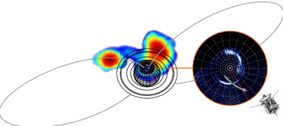
Figure caption : Schematic view of Saturn’s auroral emissions. Auroral radio emissions observed above the atmosphere were remotely mapped from Cassini (most intense emissions in red) when the spacecraft encountered a low frequency radio source. The magnetic field lines hosting it, sampled in situ by the probe, map to the (atmospheric) ultraviolet auroral oval, as observed simultaneously by the Hubble Space Telescope from Earth.
Title: The low frequency source of Saturn’s Kilometric Radiation
Authors: L. Lamy1*, P. Zarka1, B. Cecconi1, R. Prangé1, W. S. Kurth2, G. Hospodarsky2, A.
Persoon2, M. Morooka3, J.-E. Wahlund3, G. J. Hunt4
Affiliations:
1LESIA, Observatoire de Paris, Université PSL, CNRS, Sorbonne Université, Université Paris
Diderot, Sorbonne Paris Cité, 5 Place Jules Janssen, 92195 Meudon, France.
2Department of Physics and Astronomy, University of Iowa, Iowa City, IA 52242, USA.
3Swedish Institute of Space Physics, Box 537, SE-751 21 Uppsala, Sweden.
4Blackett Laboratory, Imperial College London, London, SW7 2BW, UK.
*Correspondence to: laurent.lamy@obspm.fr
Abstract:
Understanding the generation of planetary auroral radio emissions, the powerful non-thermal radiations produced by all the magnetized planets explored so far, and actively searched from exoplanets and more massive objects, requires in situ measurements from within their source region. During the ring-grazing high-inclination orbits spanning late 2016 to early 2017, the Cassini spacecraft sampled at three occasions the top of Saturn’s Kilometric Radiation (SKR) emission region, whose intensifications have long been used as a sensitive proxy of large-scale magnetospheric dynamics, providing unique in situ wave and plasma measurements. Narrow-banded radio sources were crossed at frequencies of 10-20 kHz, all in the northern dawn-side sector. They hosted extraordinary mode emission, radiated quasi-perpendicularly to the local magnetic field from 6-12 keV electron-beams consistent with the Cyclotron Master Instability and embedded within regions of upward currents themselves coincident with the main auroral oval. Overall, the SKR low frequency sources appear to be strongly controlled by time-variable electron densities.
One Sentence Summary:
The low frequency (10-20 kHz) sources of Saturn Kilometric Radiation crossed by the Cassini probe are triggered by 6-12 keV electrons and controlled by time-variable electron densities.
Main Text: Introduction
During its early 2008 high-inclination passes, the Cassini mission unexpectedly sampled two low frequency (LF) sources of Saturn’s Kilometric Radiation (SKR), generally observed over the
1-1000 kHz spectral range, and thus provided the first insights into the generation of intense non-thermal auroral radio emission at a planet other than Earth (1). The combined analysis of radio, plasma and magnetic field in situ measurements validated the Cyclotron Maser Instability (CMI), at the origin of Auroral Kilometric Radiation (AKR) at Earth, as a universal generation mechanism able to operate in different planetary magnetospheres. The CMI is a wave-electron resonant interaction which requires (1) non-maxwellian weakly relativistic electrons (whose distribution function displays a positive gradient along the velocity direction perpendicular to the
magnetic field) and (2) a ratio of the electron plasma frequency fpe overthe electron cyclotron
frequency fce much lower than unity. When these two conditions are fulfilled, radio emission is
amplified mainly on the right-hand extraordinary (R-X) mode at the frequency fCMI =
fce/Γ+k//v///2π, where k is the wave vector, v the electron velocity, // refers to the direction
parallel to the magnetic field and Γ = (1-v2/c2)-1/2 is the Lorentz factor (2). Waves are thus
amplified at the local relativistic electron cyclotron frequency Doppler shifted by the parallel
propagation. At first order, this expression thus reduces to fCMI ~ fce.
A first SKR source was identified on day 2008-291 (Oct. 17th) at ~10 kHz (i.e. ~5 RS distance,
where 1 RS = 60268km is Saturn’s radius), at the unusual Local Time (LT) of 01:00 and along
-80° invariant latitude magnetic field lines, reminiscent of spiral-shaped auroral storms arising from the midnight sector. It occurred during a global SKR intensification extending to low frequencies with wave intensities of a few mV/m, coincident with unusually strong upward-directed field-aligned currents indicative of down-going electron-beams, and was attributed to a major solar wind-driven compression of the magnetosphere (3-5). The R-X mode source was
identified from measurements of its low frequency cutoff fskr about 2% below fce. Radio waves
displayed strong linear polarization at the source from which they were radiated
quasi-perpendicularly to the local magnetic field. In this case, fskr can be expressed as fCMI = fce
(1-v2/c2)1/2 and direct measurements of fskr yielded CMI-resonant electrons of 6-9 keV in perfect
agreement with the hot (accelerated) electrons simultaneously detected in situ. Their measured shell-like 3D distribution function (referred to as horseshoe in 2D) was fully consistent with CMI-driven perpendicular emission. Sampling down-going electrons with shell-type distribution additionally implies that they had been accelerated toward the planet in regions located farther than the radio source along the flux tube (3,6-7). A second direct confirmation of the CMI mechanism was brought by the agreement between the wave properties observed within the source region and the simulated CMI wave growth rate and emission angle driven by the electron distribution measured simultaneously (8). As at Earth, the auroral plasma surrounding the
emission region was hot, with a marginal cold component, and tenuous with fpe/fce ~ 0.1 (9). On
the other hand, terrestrial-like plasma cavities were not observed within the radio source at the 2 s resolution of Cassini’s electron measurements. This difference, together with the presence of SKR sources at larger distances from the planet than AKR at Earth, was attributed to the faster rotation of Saturn's magnetosphere, which means that CMI condition (2) is generally fulfilled at high latitudes without needing small-scale cavities.
A second SKR source was likely traversed as well on day 2008-073 (March 13th) at ~5 kHz (i.e.
~6 RS distance) (10-11) The LF emission tangentially approached the fce curve on the
corresponding dynamic spectrum (time-frequency map of wave flux density) at a more usual location, near 07:30 LT, close to the SKR peak intensity region (12), and along -77° invariant
(2). The authors did not measure the low frequency cutoff fskr but again used the observed
shell-like electron distribution at about 7 keV to calculate CMI wave growth rates compatible with the observed SKR R-X mode flux densities.
This limited set of events does not provide a comprehensive view of SKR LF sources and the conditions in which the CMI can trigger them. Their understanding is however essential since intensifications of SKR spectrum in general, and of its low frequency component in particular, have long been used as a sensitive diagnostic of large-scale magnetospheric dynamics, including the SKR dual rotational modulation or night-side plasmoid ejection and associated auroral storms induced or not by the solar wind (13-24). The ultimate high-inclination phase of the Cassini mission carrying the spacecraft to high latitudes at low altitudes provided an ideal occasion to tackle these questions. It started with the ring-grazing orbital sequence, during which the spacecraft repeatedly sampled the top of both northern and southern SKR emission regions, at distances corresponding to the SKR lowest frequencies. In this study, we present a survey of these orbits, extract the average properties of the crossed radio sources and discuss the magnetospheric parameters which control them.
Survey of ring-grazing orbits
The 20 ring-grazing orbits (orbits 251 to 270), whose perikrone lies outside the F-ring, were
executed between days 2016-335 (Nov. 30th) and 2017-112 (Apr. 22nd), and sampled auroral
field lines expected to host SKR sources radiating up to 30 kHz (40 kHz) in the dawn-side northern (dusk-side southern) hemisphere, as illustrated in supplementary Figure S1. They were
preceded by 7 orbits (orbits 244 to 250) starting on day 2016-270 (Sep. 26th) which brought the
spacecraft to high latitudes and at distances close enough to the planet to probe SKR sources at a few kHz as well. We conducted a survey of kilometric sources crossed over these 27 orbits thanks to combined observations of the Radio and Plasma Wave experiment (RPWS; 25) and the magnetometer (MAG; 26).
The lack of in situ measurements of low energy electron distribution functions from the Cassini Plasma Spectrometer (CAPS; 27) after 2012 prevented the identification of SKR sources from the direct analysis of simultaneous radio and electron measurements based on growth rate calculation. Instead, on the basis of the reference event of day 2008-291, SKR sources were identified solely from RPWS/HFR (High Frequency Receiver) and MAG data whenever (i) the
emission LF cutoff fskr passed strictly below fce (ii) for at least 2 consecutive RPWS/HFR 16-s
measurements. Criterion (i) rests upon the assumption perpendicular emission which we will later show to be valid. Criterion (ii) was aimed at being conservative and avoid false detections
induced by spiky signals. The method used to determine fskr (3) is described in the supplementary
material. Overall, the survey revealed only 3 events which unambiguously fulfilled these two
criteria. All occurred in the northern hemisphere on days 2016-339 (Dec. 4th), 2016-346 (Dec.
11th) and 2017-066 (Mar. 7th), hereafter labelled as events S1, S2 and S3. No source was found in
the southern hemisphere. We rejected several candidate northern SKR sources where the LF
emission region was clearly tangent to fce but which did not fulfill criterion (ii), for instanceon
days 2016-332 (Nov. 27th) or 2017-016 (Jan. 16th). These may be either nearby sources (close to
but not crossed by Cassini) or crossings of small-sized sources lasting less than 16 s (~200-300
km for typical spacecraft velocity) and/or emission produced at fCMI > fce, as in the case of
Events S1, S2 and S3 were sampled during intervals of relatively quiet solar wind activity (C. Tao
and T. Kim, personal communication). In addition, events S1 and S2 occurred close to the
predicted rotational peak of northern SKR bursts while event S3 was rather in anti-phase with it
(1). The first two events were thus consistent with rather standard auroral activity, while the latest one indicated a more unusual case, possibly driven by internal dynamics. The detailed wave properties and characteristics of the 3 identified sources are listed in table 1 and analyzed
hereafter, on the basis of the most illustrative examples of events S3 and S1. A polar projection of
the sources of these events is provided in Figure S2. Event S3 displayed the most intense radio
emission and benefited from coordinated observations of the northern ultraviolet (UV) aurorae
by the Hubble Space Telescope (HST), while event S1 could be sampled by RPWS/WBR
waveform measurements (Wideband Receiver), the first ever obtained within a SKR source.
Examples of SKR source crossings
Radio, plasma and magnetic field measurements during events S3 and S1 are compared in Figures
1 and 2, respectively, with identical formats. SKR is the patchy bright emission observed above 10 kHz in panel A (dynamic spectrum of the wave Poynting flux S), with dominant right-handed (RH) circular polarization in panel B (dynamic spectrum of the normalized degree of circular polarization V) indicative of northern R-X mode. Some weaker left-handed (LH) polarized SKR, indicative of left-hand ordinary (L-O) mode, was additionally observed at the low frequency edge of the R-X mode SKR on the right-hand side of each interval, preceding the perikrone. The weakly polarized emission visible below 10 kHz after 15:30 UT on Figure 1A-B is identified as auroral hiss. Narrow-banded long-duration and drifting short-duration emissions observed below 35 kHz are not considered in this study (28-29). Localized SKR R-X mode LF emission is
tangent to fce near the middle of each interval. Condition fskr < fce (panel C) is then used to
precisely define the overall extent of the source region (orange-shaded area, extended by vertical
dotted-dashed lines on the other panels). During event S3 (Figure 1A-C), a single SKR source
was continuously observed from 15:11:48 to 15:17:25 UT, corresponding to a 6050 km distance
along the spacecraft trajectory. During event S1 (Figure 2A-C), multiple SKR sources were
observed between 08:42:50 and 08:59:54 UT.
Figure 3 shows dynamic spectra zooming on Figure 2A at unprecedented time-frequency resolution thanks to RPWS/WBR waveform measurements. Faint, localized, remote SKR
emissions observed well above fce (panel A) display recurrent drifting sub-structures with
positive and (mostly) negative rates of ~1 kHz/min, in agreement with previous SKR waveform observations (30). Their analysis is beyond the scope of this study. A zoom in on the 08:00-09:10 interval (panel B) reveals the time-frequency structure of the encountered radio source. While Figure 3A suggested a single emission pattern with a bandwidth of a few kHz lasting for nearly 2 h, Figure 3B shows that it actually splits into several sub-components of variable durations and
bandwidths. Those with frequencies slightly, but clearly, above fce likely correspond to sources
on nearby flux tubes, while only the component strictly tangent to and below fce indicates a local
source. The overplotted red fskr profile(as determined in Figure 2C) provides, despite its 16 s
temporal resolution, a one-to-one correspondence between the brief episodes of fskr < fce and the
observed SKR bursts (be it the central one between 08:45 and 08:50 or the shorter ones beside it)
here observed at a 1-s cadence. This agreement validates the method employed to determine fskr
to the point that, for this specific event, we considered non-consecutive RPWS/HFR episodes
9 SKR sub-sources. Their horizontal size along the spacecraft trajectory, and across the encountered flux tubes, ranges from 240 to 3400 km. Their ~100-400 Hz bandwidth Δf
characterizes very narrow-banded emissions with Δf/fce ~ 0.008-0.03, and thus correspond to
radiating structures which extended vertically ~700-2800 km along the magnetic flux tubes.
Perpendicular emission and energy of source electrons
On the right-hand side of Figures 1-2C is displayed a scale providing the energy of CMI-unstable
electrons associated with the measurements of fskr < fce, assuming perpendicular emission at the
source and thus fskr = fce(1-v2/c2)1/2, as observed during the southern event of 2008-291. To check
this assumption, we analyzed the wave parameters derived from the goniopolarimetric analysis of RPWS/HFR 3-antenna measurements (see the supplementary material for details). These consist of the wave Stokes parameters S, Q, U and V (as displayed on Figures 1-2 and S3) and the k-vector direction. From the latter were can additionally retrieve the 3D locus of the radio
source, from the intersection of the k line-of-sight with a model iso-f=fce surface (assuming
straight-line propagation, which is reasonable at high latitude), and its beaming angle θ = (k,B), where B is the magnetic field vector at the source (31,3,7,12).
Figure 4 displays the variation of the beaming angle θ(f) of events S3 and S1 for the time
intervals of Figures 1-2 using a standard data selection with red (blue) symbols corresponding to RH (LH) polarized waves, and thus to R-X (L-O) mode. The solid colored lines provide the median value of θ at each frequency for which the number of crosses (exact determination of the source position) exceeds the number of diamonds (approximated determination of the source position). In agreement with previous studies of the SKR beaming angle (1 and refs therein), θ(f) of R-X mode emission smoothly rises from ~60°±25° at ~800 kHz to >85°±15° at 30 kHz, the uncertainty on θ being dominated by the scattering of data points. Supplementary figure S3E shows an alternative representation of θ(f) in the time-frequency plane. This systematic change from perpendicular to oblique emission with increasing frequency may be primarily due to
refraction of R-X mode waves on the nearby iso-fX surface, where fX ~ fce is the R-X mode cutoff
frequency, as proposed for auroral radio emissions of the Earth and Jupiter (32-33). In this case, the apparent R-X mode beaming angle should vary as a function of the k-vector direction projected in a plane perpendicular to B, with strongest refraction expected for wave propagation toward the equator. Interestingly, L-O mode SKR was also observed, over an extended spectral range of 20-100 kHz, with θ(f) remaining confined above 75° and with a lower scattering than
the R-X mode one. Indeed, the L-O mode cutoff frequency being fpe, which was here much lower
than fce (see Figures 1-2D), no similar refraction on the iso-fO surface is expected. This
interpretation, whose validation is beyond the scope of this study, thus implies that θ(f) measures in fact the apparent (real) beaming angle of SKR R-X (L-O) mode affected (unaffected) by refraction. Although they differ at high frequencies, both remote observations of R-X and L-O mode θ(f) indicate quasi-perpendicular emission at 30 kHz, toward frequencies where the local radio sources have been sampled.
A second method providing a direct measurement of the wave emission angle within the source rests upon its polarization state. Indeed, for perpendicular cyclotron emission, the polarization
ellipse ratio AR = (T1/2 – L)/V, with T = (Q2+U2+V2)1/2 and L = (Q2+U2)1/2 being the total and
linear polarization degrees (34), can be approximated by cos θ at first order (35). Figures 1-2B and Figure S3A-D show that the emission is indeed strongly linearly polarized at the source, again as it had been observed during the southern event of day 2008-291. Measurement of the
encompassing fce with standard data selection (SNR > 20 dB, T > 0.85, |zr| < 0.2) gives AR =
-0.05±0.15, -0.07±0.27 and -0.02±0.26, which results in θ = 93±9°, 86±16° and, 91±16° respectively, all fully consistent with perpendicular emission.
The measured values of fskr can now be safely inverted to derive energies of CMI-unstable
electrons, as summarized in table 1 and illustrated in Figure 1-2C. In average, fskr reached a -2%
level below fce with an extremum at -3.5%. The corresponding electron energies spanned the
1-17keV range, with mean values between 6 and 12 keV depending on the event and a standard
deviation of a 3-4 keV, larger than the 2 keV resolution arising from the accuracy of fskr. We did
not notice any correlation between the obtained electron energies and the observed wave intensities, measured between a few 0.01 and a few mV/m.
Auroral plasma conditions
We now investigate the auroral plasma conditions to assess the validity of CMI condition (2).
Figures 1-2 D display the characteristics frequencies fskr (solid line), fce and fce/10 (dashed lines)
together with fpe (colored lines). fpe was derived from Langmuir Probe (LP) 32-s measurements
(gray profile) and compared to the upper frequency cutoff of auroral hiss (red profile) derived independently from the RPWS/MFR (Medium Frequency Receiver) 64-s measurements. The LP measures the total electrical current carried by the ambient plasma from voltage sweeps, from
which the electron density Ne and thus fpe are derived. Here, the voltage sweep resolution implies
a typical uncertainty on fpe less than a factor of 2. Auroral hiss is a whistler-mode emission
radiated upward from below the spacecraft and propagating beneath fpe, so that its upper
frequency cutoff, when marking a sharp transition, is a proxy of fpe when fpe < fce. Here, the
observed hiss emissions were generally damped and exhibited a smoothed cutoff so that the
fitted frequencies were rather interpreted as a lower limit of fpe, labelled fpe min. These two
methods are described in more details in the supplementary material. On Figures 1-2 D, the fpe min
profiles in red were indeed close to and generally below the LP-derived fpe profilesin gray. For
event S1, fpe/fce was about 0.03 across the whole source region, which exactly ended when the
value of fpe (fpe min) suddenly rose by a factor of 4 (13) at 15:18 UT (15:20), overcoming the
fce/10 threshold for CMI condition (2). For event S3, a similar density gradient was observed in
both datasets. The hiss cutoff frequency fpe min rose by a factor of 5 at 09:04, again shortly after
the SKR source region at 09:00. The LP-derived fpe, determined with a time resolution twice
better, reveals more complex variability: while fpe rose by a factor of 4 at 08:42, it then showed
large-scale fluctuations of a factor of ~3 (~2) up to (after) 09:00. Interestingly, the SKR
sub-sources (sampled at a better cadence) strikingly match the local minima of fpe, suggesting that
small-sized radio sources were possibly co-located with density cavities. During event S2,the
LP-derived fpe was obtained with too low time resolution to provide any reliable estimate of
fpe/fce.
Figures 1-2 E show the azimuthal component of the magnetic field measured from 1-min averaged MAG data. They indicate upward currents in intervals dominated by a positive slope, the main one being marked by a green-shaded region. Each SKR source region precisely started at (but ended before) the beginning (the end) of the upward current region. The upward current
density was estimated to 106, 171 and 157 nAm-2 for events S1, S2 and S3, respectively, well
above the average of 80 nAm-2 derived from all the ring-grazing northern upward current regions
Additional information on the correspondence between auroral emissions and upward currents is
brought by Figure 5, which maps the spatial distribution of SKR sources during event S3 together
with that of northern UV aurorae simultaneously observed by HST on 2017-066 (Mar. 17th) over
15:27-16:21 UT (light-time corrected). Panel (A) displays the distribution of SKR emissions observed over the same time interval as Figure 1 in the plane of sky as seen from Cassini. The displayed data, definition of symbols and color scales are similar to Figure 4A, except that the
data selection was here more restrictive for clarity. As expected from emission close to fce
(directly proportional to |B|), SKR lower (higher) frequency sources are observed at larger (closer) distances from the planet. Panel (B) displays in a polar view the magnetic footprint of radio sources visible in panel (A). Dotted-dashed lines indicate radio horizons at extremal frequencies, beyond which no radio source can in principle be observed. The R-X mode footprints (in red) draw a clear circumpolar auroral oval visible from 04:00 to 22:00 LT. Its large latitudinal width of about 8-10° is dominated by the scattering of goniopolarimetric results. This extended range derives from the LT range swept by the spacecraft (green double arrow) during the investigated interval. Movie 1 displays an animation of panels (A-B) and illustrates how the spatial distribution of detected sources varies with the time-variable position of the spacecraft. The L-O mode footprints (in blue) are well clustered and precisely co-located with the R-X mode ones between 08:00 and 10:00 LT. The comparison with panel (D) illustrates that SKR sources are strikingly co-located with the UV auroral oval (see Figure S4 for a superimposition of both panels), both on the dawn-side sector, where the UV oval is thin and well defined between 06:00 and 12:00 LT from +72° to +75° latitudes, and on the dusk-side sector, with UV aurorae more spread in latitude between 14:00 and 23:00 LT and including a poleward arc beyond +80° between 14:00 and 18:00 LT. The Cassini footprint trajectory is displayed on panels B-D over the 13:00-17:00 UT interval by the gray line. The green and red (overlapping) portions of it refer to the upward current region and the SKR source region identified in Figure 1. The upward current layer exactly matches the main UV auroral oval in size while the SKR source was crossed along a smaller, poleward, portion of it. This can be better seen in panel (C), which is similar to (B) except that it restricts to the crossed SKR source component with slightly relaxed data selection to improve statistics (the supplementary material discusses the reliability of direction-finding results for strongly linearly polarized emissions such as those observed here). Again, the footprints of R-X mode located sources nicely map to the red portion of Cassini’s trajectory and only to the inward portion of the main oval and associated upward current layer.
Discussion
We now discuss the average properties of SKR LF emissions as a whole in the CMI frame. The identification of solely 3 SKR sources in the dawn-side sector and none in the dusk-side sector brings a direct in situ confirmation to the LT dependence of SKR spectrum (here observed during quiet solar wind conditions), with lowest frequencies at dawn (15,23). The small number of radio sources identified along orbits with very similar trajectories and their limited extent additionally reveal time-variable generation conditions.
In all three cases, the sampled R-X mode emission was found to be amplified nearly
perpendicularly to the local magnetic field, with emission frequency clearly below fce supplied
by CMI-unstable electrons of 6-12 keV mean energies. Direct perpendicular emission through CMI additionally requires specific shell-type distribution functions of the accelerated electrons in the phase plane such as those already measured for the 2 southern SKR sources crossed in 2008
(8,11). The kronian situation thus directly compares to the terrestrial case, where AKR sources are commonly found to be associated with trapped or shell/horseshoe/ring distributions
(2,37-38). It differs from the situation investigated in situ by Juno at Jupiter, where the hectometer and
decameter emissions appear to be produced at oblique angles from the local magnetic field by loss cone electron distribution functions (39-40). The presence of 6-12 keV electron-beams with
such distribution functions at 3.5-4.5 RS distances from Saturn’s center, or equivalently 2.8-3.7
RS from the atmosphere along the encountered flux tubes (see table 1), imply that at least part of
the acceleration by upward currents occurred farther along the field lines, which provide further constraints to models of current-voltage relationships (41).
The general agreement with the CMI mechanism relies on the fulfilling of both CMI conditions mentioned in the introduction. This is first worth noting that the 3 encountered SKR sources matched upward currents with current densities larger than the average, consistent with an acceleration region extending to higher altitudes and thus satisfying CMI condition (1). We then noticed that, while the spacecraft entered the northern SKR source region when it encountered an
upward current region, it exited it when fpe suddenly rose, exceeding the typical fce/10 threshold.
After exiting the source, the spacecraft remained for some time inside the upward current region itself precisely mapping to the main UV oval across the Cassini trajectory. This suggests that at
3.5-4.5 RS distances, SKR emission is primarily controlled by the electron plasma density Ne
through CMI condition (2) which quenches the radiation when fpe/fce typically exceeds 0.1.
According to the Knight relationship (42) and assuming a constant current density, larger Ne is
also expected to decrease electron acceleration and weaken CMI condition (1).
Figure 6 displays radio, plasma and magnetic measurements in format identical to Figure 1 A,D-E for 3 successive, quasi-identical, passes of the spacecraft in the northern dawn-side auroral
region : the middle panels correspond to event S3 investigated in Figure 1 (orbit 264), while the
right and left-handed panels correspond to the previous (orbit 263) and the following (orbit 265) auroral passes. The probe did not fly across any local SKR source during orbit 263 and 265 while it encountered regions of upward current in all cases (green-shaded regions) with current
densities of 29 and 108 nA m-2, again mapping to the main UV auroral oval (the HST
observation obtained during orbit 265 is not shown). On orbit 265, the SKR intensity was relatively bright and its spectrum reached low frequencies down to 20 kHz, while the upward current density was as strong as that of orbit 264. Instead, on orbit 263, SKR was comparatively fainter with a spectrum confined to higher frequencies and a lower upward current density. This
suggests that CMI condition (1) requiring unstable electrons at 3.6 RS was plausible for orbit 265,
at least. For both intervals though, fpe was systematically larger than fce/10 within the upward
current region, in contrast with orbit 264 (event S3), therefore revealing that the mean level of Ne
over hours-long interval significantly varies with time from pass to pass. This further shows that CMI condition (2) was not fulfilled for any of orbits 263 and 265 and possibly quenched any SKR LF emission during orbit 265.
The origin of time-variable plasma densities at the altitude of LF SKR sources has now to be identified. The asymmetrical plasmapause-like boundary, this transition from high to low plasma densities with increasing latitudes which rotates at the northern SKR period, is a plausible source
for time-variable Ne (43). On a shorter timescale, Figure 1 does not display any Earth-like
plasma cavity, as already noticed for the 2008-291 southern event. However, Figure 2
interestingly shows small-sized, recurrent, drops of fpe co-located with SKR sources for event S1
Earth. Definite conclusions however rely on knowing whether the plasma region was dominated by hot electrons (such as on day 2008-291) or could have included a significant cold plasma component sensitive to local potential drops and able to map plasma cavities. As the CAPS experiment was not operating during these orbits, these questions remain open.
Finally, the very narrowbanded nature of SKR sources noticed escpecially during event S1 is
consistent with either a non-saturated linear wave growth, as predicted by the CMI theory and measured in laboratory (e.g. 44), or with saturation by coherent non-linear trapping previously assumed to correctly model the SKR spectrum (45). However, the emission levels may be too low to even reach saturation and the observed wave intensities (table 1) are rather consistent with linear growth.
This study of SKR LF sources will form a basis to similarly analyze the Cassini proximal orbits, in which the spacecraft sampled the peak of SKR spectrum at lower altitudes (see Figure S1).
References and Notes:
1. L. Lamy, The Saturnian Kilometric Radiation before the Cassini Grand Finale. In Planetary
Radio Emissions VIII, edited by G. Fischer, G. Mann, M. Panchenko, and P. Zarka, Austrian
Academy of Sciences Press, Vienna, 171–190 (2017).
2. R. A. Treumann, The electron-cyclotron maser for astrophysical applications. Astron. Astrophys. Rev., 13, 229-315 (2006). doi:10.1007/s00159-006-0001-y
3. L. Lamy et al., Properties of Saturn kilometric radiation measured within its source region.
Geophys. Res. Lett., 37, L12104 (2010). doi:10.1029/2010GL043415
4. E. J. Bunce et al., Extraordinary field-aligned current signatures in Saturn’s high-latitude magnetosphere: Analysis of Cassini data during revolution 89. J. Geophys. Res., 115, A10238 (2010). doi:10.1029/ 2010JA015612
5. W. S. Kurth et al., A close encounter with a Saturn kilometric radiation source region. In
Planetary Radio Emissions VII, edited by H. O. Rucker, W. S. Kurth, P. Louarn and G.
Fischer, Austrian Academy of Sciences Press, Vienna, 75–85 (2011).
6. P. Schippers et al., Auroral electron distributions within and close to the Saturn kilometric radiation source region. J. Geophys. Res., 166, A05203 (2011). doi:10.1029/2011JA016461 7. L. Lamy et al., Emission and propagation of Saturn kilometric radiation: Magnetoionic
modes, beaming pattern, and polarization state. J. Geophys. Res., 116, A04212 (2011). doi:10.1029/2010JA016195
8. R. L. Mutel et al., CMI growth rates for Saturnian kilometric radiation, Geophys. Res. Lett., 37, L19105 (2010). doi:10.1029/2010GL044940
9. A. Hilgers, The auroral radiating plasma cavities, Geophys. Res. Lett., 19, 3, 237-240 (1992).
doi: 10.1029/91GL02938
10. J. D. Menietti et al., Saturn kilometric radiation near a source center on day 73. In Planetary
Radio Emissions VII, edited by H.O. Rucker, W. S. Kurth, P. Louarn, and G. Fischer,
Austrian Academy of Sciences Press, Vienna, 87–95 (2011).
11. J. D. Menietti, R. L. Mutel, P. Schippers, S.–Y. Ye, D. A. Gurnett, L. Lamy, Analysis of Saturn kilometric radiation near a source center. J. Geophys. Res., 116, A12222 (2011). doi:10.1029/2011JA017056
12. L. Lamy, B. Cecconi, R. Prange, P. Zarka, J. D. Nichols, and J. T. Clarke, An auroral oval at the footprint of Saturn’s kilometric radio sources, colocated with the UV aurorae. J.
Geophys. Res., 114, A10212 (2009). doi:10.1029/2009JA014401
13. W. S. Kurth et al., An Earth-like correspondence between Saturn’s auroral features and radio emission. Nature, 433, 722-725 (2005). doi:10.1038/nature03334
14. W. S. Kurth et al., Saturn kilometric radiation intensities during the Saturn auroral campaign of 2013. Icarus, 263, 2–9 (2016). doi:10.1016/j.icarus.2015.01.003
15. L. Lamy, P. Zarka, B. Cecconi, R. Prangé, W.S. Kurth, and D.A. Gurnett, Saturn kilometric radiation: Average and statistical properties. J. Geophys. Res., 113, A07201 (2008). doi:10.1029/2007JA012900.
16. S. V. Badman, S. W. H. Cowley, L. Lamy, B. Cecconi, P. Zarka, Relationship between solar wind corotating interaction regions and the phasing and intensity of Saturn kilometric radiation bursts. Ann. Geophys., 26, 3641–3651 (2008).
17. D. A. Gurnett et al., Discovery of a north-south asymmetry in Saturn’s radio rotation period.
Geophys. Res. Lett., 36, L16102 (2009). doi:10.1029/2009GL039621
18. D. G. Mitchell et al., Recurrent energization of plasma in the midnight-to-dawn quadrant of Saturn’s magnetosphere, and its relationship to auroral UV and radio emissions. Plan. Sp.
Sci., 57 (2009) 1732–1742 (2009). doi:10.1016/j.pss.2009.04.002
19. C. M. Jackman et al., On the character and distribution of lower-frequency radio emissions at Saturn and their relationship to substorm-like events. J. Geophys. Res., 114, A08211 (2009). doi:10.1029/2008JA013997
20. C. M. Jackman et al., In situ observations of the effect of a solar wind compression on Saturn’s magnetotail. J. Geophys. Res., 115, A10240 (2010). doi:10.1029/2010JA015312 21. L. Lamy, Variability of southern and northern SKR periodicities. In Planetary Radio
Emissions VII, edited by H.O. Rucker, W.S. Kurth, P. Louarn, and G. Fischer, Austrian
Academy of Sciences Press, Vienna, 39–50 (2011).
22. L. Lamy et al., Multispectral simultaneous diagnosis of Saturn’s aurorae through- out a planetary rotation, J. Geophys. Res., 118, 4817–4843 (2013).
23. T. Kimura et al., Long-term modulations of Saturns auroral radio emissions by the solar wind and seasonal variations controlled by the solar ultraviolet flux. J. Geophys. Res., 118, 7019– 7035 (2013).
24. J. J. Reed, C. M. Jackman, L. Lamy, W. S. Kurth, D. K. Whiter, Low Frequency Extensions of the Saturn Kilometric Radiation as a proxy for magnetospheric dynamics. J. Geophys.
Res., in press (2018). doi:10.1002/2017JA024499
25.D. A. Gurnett et al., The Cassini Radio and Plasma Wave Investigation. Sp. Sci. Rev., 114,
395-463 (2004). doi:10.1007/978-1-4020-2774-1_6
26.M. K. Dougherty et al., The Cassini magnetic field investigation. Sp. Sci. Rev., 114, 331-383
(2004). doi:10.1007/s11214-004-1432-2
27. D. T. Young et al., Cassini Plasma Spectrometer investigation. Space Sci. Rev., 114, 1–112 (2004). doi:10.1007/s11214-004-1406-4
28. S.-Y. Ye et al., Source locations of narrowband radio emissions detected at Saturn. J. Geophys. Res., 114, A06219 (2009). doi:10.1029/2008JA013855
29. U. Taubenschuss, J. S. Leisner, G. Fischer, D. A. Gurnett, F. Nemec, Saturnian low frequency drifting radio biursts : statistical properties and polarization. In Planetary Radio
Emissions VII, edited by H.O. Rucker, W.S. Kurth, P. Louarn, and G. Fischer, Austrian
Academy of Sciences Press, Vienna, 115-123 (2011)
30. W. S. Kurth et al., High spectral and temporal resolution observations of Saturn kilometric radiation, Geophys. Res. Lett., 32, L20S07 (2005).
31. B. Cecconi, L. Lamy, P. Zarka, R. Prangé, W. S. Kurth, P. Louarn, Goniopolarimetric study of the revolution 29 perikrone using the Cassini Radio and Plasma Wave Science instrument high-frequency radio receiver. J. Geophys. Res., 114, A03215 (2009). doi 10.1029/2008JA013830
32. R. L. Mutel, I. W. Christopher, J. S. Pickett, Cluster multispacecraft determination of AKR angular beaming. Geophys. Res. Lett., 37, L07104 (2008). doi :10.1029/ 2008GL033377 33. P. H. M. Galopeau, M. Y. Boudjada, An oblate beaming cone for Io-controlled Jovian
decameter emission. J. Geophys. Res., 121, 3120–3138 (2016). doi:10.1002/2015JA021038. 34. J. D. Kraus, Wave polarization. In Radio Astronomy, 116–125, McGraw-Hill, New York
(1966).
35. D. B. Melrose, G. A. Dulk, On the elliptical polarization of Jupiter’s decametric radio emission. Astron. Astrophys., 249, 250–257 (1991).
36. G. J. Hunt, G. Provan, E. J. Bunce, S. W. H. Cowley, M. K. Dougherty, and D. J. Southwood, Field-aligned currents in Saturn’s magnetosphere: Observations from the F-ring orbits. J. Geophys. Res., in press.
37. P. Louarn, A. Roux, H. de Féraudy, D. Le Quéau, M. André, L. Matson, Trapped electrons as a free energy source for the auroral kilometric radiation. J. Geophys. Res., 95, 5983-5995, (1990). doi:10.1029/JA095iA05p05983
38. R. E. Ergun,C. W. Carlson, P. McFadden,G. T. Delory,R. J. Strangeway, P. L. Pritchett,
Electron-Cyclotron Maser Driven by Charged-Particle Acceleration from Magnetic Field
alignedElectricFields. The Astrophys. J., 538:456-466 (2000).
39. P. Louarn et al., Generation of the Jovian hectometric radiation: First lessons from Juno,
Geophys. Res. Lett., 44, 4439–4446, (2017). doi:10.1002/2017GL072923
40. C. K. Louis et al., Io-Jupiter decametric arcs observed by Juno/Waves compared to ExPRES simulations, Geophys. Res. Lett., 44, (2017). doi:10.1002/2017GL073036
41. L. C. Ray, M. Galand, P. A. Delamere, B. L. Fleshman, Current-voltage relation for the Saturnian system, J. Geophys. Res. Space Physics, 118, 3214–3222 (2013). doi:10.1002/jgra.50330
42. S. Knight, Parallel electric fields. Planet. Space Sci., 21, 741–750 (1973).
43. D. A. Gurnett, A. M. Persoon, J. B. Groene, W. S. Kurth, M. Morooka, J.-E. Wahlund, and J. D. Nichols, The rotation of the plasmapause-like boundary at high latitudes in Saturn’s magnetosphere and its relation to the eccentric rotation of the northern and southern auroral
ovals. Geophys. Res. Lett., 38, L21203 (2011). doi:10.1029/2011GL049547.
44. R. Bingham et al., Laboratory astrophysics: Investigation of planetary and astrophysical maser emission, Sp. Sci. Rev., 178, 695-713 (2013).
45. P. H. M. Galopeau, P. Zarka, and D. Le Quéau, Theoretical model of Saturn’s kilometric radiation spectrum. J. Geophys. Res., 94, 8739–8755 (1989).
46. L. J. Davis, E. J. Smith, A model of Saturn’s magnetic field based on all available data. J.
Geophys. Res., 95, 15,257–15,261 (1990).
47. J. E. P., Connerney, M. H. Acuna, N. F. Ness, Currents in Saturn’s magnetosphere, J.
Geophys. Res., 88, 8779–8789 (1983).
48. L. Lamy, R. Prangé, F. Henry, P. Le Sidaner, The Auroral Planetary Imaging and
Spectroscopy (APIS) service. Astron. and Comp., 11, 138–145 (2015).
doi:10.1016/j.ascom.2015.01.005
49. J.-C. Gérard, B. Bonfond, J. Gustin, D. Grodent, J. T. Clarke, D. Bisikalo, V. Shematovich, Altitude of Saturn’s aurora and its implications for the characteristic energy of precipitated
electrons. Geophys. Res. Lett., 36, L02202 (2009). doi:10.1029/2008GL036554
50. J. Gustin, B. Bonfond, D. Grodent, J.-C. Gérard, Conversion from HST ACS and STIS auroral counts into brightness, precipitated power, and radiated power for H2 giant planets. J.
Geophys. Res.,117, 7316 (2012). doi: 10.1029/2012JA017607
51. B. Cecconi, P. Zarka, Direction finding and antenna calibration through analytical inversion of radio measurements performed using a system of 2 or 3 electric dipole antennas. Radio
Sci., 40, RS3003 (2005). doi:10.1029/2004RS003070.
52. M. W. Morooka, R. Modolo, J.-E. Wahlund, M. André, A. I. Eriksson, A. M. Persoon, D. A. Gurnett, W. S. Kurth, A. J. Coates, G. R. Lewis, K. K. Khurana, M. Dougherty, The electron density in Saturn’s magnetosphere. Ann. Geophys., 27, 2971–2991 (2009).
53. A. M. Persoon, D. A. Gurnett, S. D. Shawhan, Polar cap electron densities from DE 1 plasma
wave observations. J. Geophys. Res., 88, 10123-10136 (1983). doi:
10.1029/JA088iA12p10123
Acknowledgments:
The used data are available from the following sources. The Cassini/RPWS and MAG original
data are accessible through the PDS archive at archived at https://pds.nasa.gov/. The HFR
processed data are available though the LESIA/Kronos database at
http://www.lesia.obspm.fr/kronos. The UV observations were obtained from the ESA/NASA
Hubble Space Telescope (GO program 14811) : the original data can be retrieved from the
MAST archive, and the processed data from the APIS service http://apis.obspm.fr hosted by
Paris Astronomical Data Centre.
The authors thank the engineering teams in charge of processing the data, in particular T. Averkamp in Iowa City and M.-P. Issartel in Meudon. The French coauthors acknowledge support from CNES and CNRS/INSU programs of Planetology (PNP) and Heliophysics (PNST). LL thanks L. Spilker and the Cassini/MAPS group for their support to the HST program coordinated with the Cassini Grand Finale, together with C. Tao and T. Kim for inputs on solar wind conditions at Saturn. The research at the University of Iowa was supported by NASA through Contract 1415150 with the Jet Propulsion Laboratory.
LL led the analysis and wrote the paper. PZ, BC and WSK helped in the analysis of HFR data, and GH in the understanding of WBR measurements. AP analyzed the MFR measurements and digitized hiss emission frequencies. MM and JEW analyzed the LP data and derived electron densities. RP contributed to the investigation of HST observations. GH calculated the current densities from MAG data. All authors discussed the results and commented on the manuscript.
Table 1. Properties of 3 R-X mode SKR low frequency sources identified during the Cassini
ring-grazing orbits. When provided, uncertainties indicate standard deviations.
Time range (UT) 2016-339 08:42:50 – 08:59:54 (orbit 251) 2016-346 13:33:26 – 13:34:30 (orbit 252) 2017-066 15:11:48 – 15:17:25 (orbit 264)
S/C latitude (°) S/C LT (h) S/C distance to Saturn’s center (Rs)
S/C altitude along the flux tube (Rs)
+61.9 – 60.9 9.06 – 9.41 4.47 – 4.31 3.65-3.49 +59.6 – 59.5 9.72 – 9.74 4.15 – 4.14 3.33-3.32 +54.0 – 53.1 10.32 – 10.43 3.63 – 3.58 2.84-2.79 fce (kHz) 13 – 14 15 22 – 23 Δf (kHz) 0.1-0.4 <1.5 <2 Size range (km) 240 – 3400 (9 sub-sources) 1300 (1 source) 6050 (1 source) Mean fskr/fce ratio (range) 0.976 ± 0.006 (0.965 – 0.998) 0.975 ± 0.008 (0.968 – 0.987) 0.989 ± 0.004 (0.978 – 0.995) Mean Ee- (keV) (range) 11 ± 3 (1 – 17) 12 ± 4 (7 – 16) 6 ± 3 (3-11) Median Poynting flux (Wm-2) (range) 5.9 10-13 (2.6 10-14 – 2.7 10 -11) 1.2 10-13 (9.1 10-14 – 1.6 10-12) 7.3 10 -12 (2.0 10-13 – 2.3 10-8)
Mean Electric field amplitude (mV/m) (range) 0.033 ± 0.032 (0.004 – 0.142) 0.014 ± 0.011 (0.008 – 0.035) 0.292 ± 0.884 (0.012 – 4.211) Beaming angle (°) θ = (k,B) 93 ± 9 86 ± 16 91 ± 16 Upward current density (nA m-2) 157 171 105
Fig. 1. Cassini radio, plasma and magnetic measurements acquired on day 2017-066 between
13:00 and 17:00 UT (event S3) in the northern dawn-side sector. The used datasets are described
in details in the supplementary material. (A and B) Dynamic spectra of wave Poynting flux S and normalized degree of circular polarization V respectively derived from 2- and 3-antenna
RPWS/HFR 16-s measurements over 3.5-1500 kHz. V = -1 (+1) refer to RH (LH) polarization, and thus to R-X (L-O) mode emission in the northern hemisphere. The white dashed lines
indicate the electron cyclotron frequency fce as derived from MAG data. R-X mode SKR around
20 kHz comes close to fce after 15:00 (C) Ratio of the SKR low frequency cutoff fskr to fce.
Values fskr/fce < 1 define one SKR source crossing between 15:11 and 15:18 (orange-shaded
region on panels C-D, extended by vertical dotted-dashed lines in the other panels). The
right-handed gray scale provides the electron energy inferred from fskr = fce(1-v2/c2)1/2 assuming
perpendicular emission. (D) Characteristic frequencies comparing fskr (solid black line), fce and
fce/10 (dashed black lines) and the electron plasma frequency fpe as directly derived from RPWS
Langmuir probe 32-s measurements (gray profile) together with a lower limit of it fpe min
estimated from the auroral hiss upper frequency cutoff measured with RPWS/MFR 64-s measurements (red profile). (E) Magnetic azimuthal component Bφ, as from 1-min averaged MAG measurements in spherical coordinates. The green-shaded region marks a region of positive slope, indicative of an upward-directed current region. The SKR source region precisely
lights up at the beginning of the upward current region and ends before Cassini exits it, when fpe
Fig. 2. Cassini radio, plasma and magnetic measurements acquired on day 2016-339 between
07:00 and 11:00 UT (event S1) in the northern dawn-side sector, in a format identical to Figure 1.
Here, 9 SKR sources near 12 kHz were successively encountered between 08:43 and 09:00. The overall interval is delimited by a light orange-shaded region, while the individual SKR sources are indicated by dark orange-shaded areas.
Fig. 3. High resolution dynamic spectra of event S1 reconstructed from Cassini radio electric
waveform measurements acquired on 2016-339. They were acquired with the RPWS/WBR receiver over the 0-80 kHz range, as described in the supplementary material. (A) Reconstructed
dynamic spectrum between 07:30 and 09:30 UT. The dashed line indicates fce. (B) Zoom on the
encountered local SKR source. The red solid line indicates fskr, as derived from RPWS/HFR
measurements in Figure 1D. It is in excellent agreement with high resolution WBR
measurements of SKR emission close to and below fce.
07:40 08:00 08:20 DOY 2016-339 (h) DOY 2016-339 (h) 08:40 09:00 09:20 0 10 20 30 40 50 60 70 80 F requency (kHz ) F requency (kHz ) 1 0- 1 6 - 1 5 1 0- 1 4 1 0 V 2m -2H z -1 08:00 08:20 08:40 09:00 10 12 14 16 18 20 - 1 5 1 0- 1 4 1 0 V 2m -2H z -1 A B fce fskr fce
Fig. 4. SKR beaming angle at the source as a function of frequency. (A) Time interval from
13:00 to 17:00 UT on 2017-066 (event S3) encompassing the SKR source crossed around 15:15.
The beaming angle is defined as θ = (k,B), where k is the wave vector determined remotely from RPWS/HFR 3-antenna measurements, and B the magnetic field vector at the source. The principle of 3-antenna measurements, the method used to derive θ and the selection criteria are described in details in the supplementary material. A standard data selection was here applied
with T > 0.85, |zr| < 0.05 and SNR±X,Z > 20 dB. The color scale refers to the wave frequency,
with red (blue) symbols corresponding to RH (LH) polarized waves and thus to R-X (L-O)
mode. Crosses (diamonds) indicate k directions which intercept (do not intercept) their iso-f=fce
surface, assuming straight line propagation. Red and blue lines indicate the median value of θ, derived at each frequency for which the number of crosses exceeds the number of diamonds (7). The dotted line marks emission perpendicular to the local magnetic field vector. (B) Time
interval from 07:00 to 11:00 UT on 2016-339 (event S1) encompassing the multiple SKR sources
crossed around 08:50. The data selection was identical to A except that SNR±X,Z > 30 dB to
better remove faint non-SKR narrow-banded emissions observed up to 40 kHz. Both panels show that θ increase from ~60° at ~800 kHz to ~80° at 30 kHz, consistent with quasi-perpendicular emission at the source.
100 SNR > 20dB 2017-066 13:00-17:00 2016-339 07:00-11:00 SNR > 30dB B A 1000 f (kHz) 100 1000 f (kHz) (°) ±X,Z ±X,Z 0 20 40 60 80 100 120
Fig. 5. Spatial distribution of SKR sources and UV aurorae. The data processing used to build
the panels is again described in details in the supplementary material. (A) 2D locus of SKR sources as seen from Cassini, from RPWS/HFR 3-antenna measurements of k directions on
2017-066 13:00-17:00 UT (event S3). The applied data selection was identical to that used in
Figure 4A, except that SNR±X,Z > 40 dB for the sake of clarity. The color scale and definition of
symbols is identical to Figure 4A. The red planetary meridian indicates noon. The typical 2° uncertainty on k measurements is displayed by the bottom-right circle. (B) Polar view of the magnetic footprint of radio sources displayed in panel A as a function of planetocentric latitude and LT. The dotted-dashed curved lines display radio horizons at extremal frequencies, beyond which a radio source cannot be observed. The double green arrow indicates the Cassini LT range swept during the interval. The gray line plots the associated Cassini magnetic footprint, whose orange and green portions indicate the crossing of SKR source and of the upward current region
24:00 12:00 06:00 18:00 +50° +70° Cassini FOV (120°) RS RS Error ellipse: 2°
Magnetic polar projections
A B radio horizon f=1000kHz radio horizon f=27kHz radio horizon f=20kHz 24:00 12:00 06:00 18:00 o o kR H2 0 10 20 30 -6 -4 -2 0 2 4 6 -6 -4 -2 0 2 4 6 f (kHz) RH/LH 100 1000 C 24:00 12:00 06:00 18:00 +50° +70° +50° +70° D f (kHz) RH 20-27
identified in Figure 1. (C) Same as B but for the SKR source observed from 09:00 to 09:20
between 20 and 27 kHz. The data selection was here slightly relaxed with T > 0.85, |zr| < 0.2 and
SNR±X,Z > 20 dB to maximize statistics. Cassini’s LT is indicated by a green dotted-dashed
arrow. The radio source footprints coincide with the crossed SKR source (orange portion of the
gray line). (D) Polar view of Saturn’s H2 aurorae observed with the Hubble Space Telescope
(using the STIS instrument and the SrF2 filter) on day 2017-066 from 15:27 to 16:21 UT, once
corrected from light-time travel. The background-subtracted image was projected onto the 1100
km altitude surface as a function of planetocentric coordinates and expressed in kR of H2. The
gray line and its colored portions are identical to B and C. The upward current layer (green) strikingly matches the main auroral oval, while the SKR source crossed (orange) only matches the poleward portion of it.
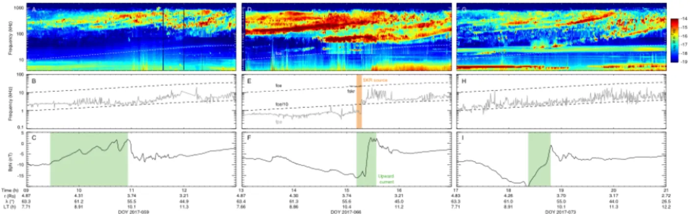
Fig. 6. Cassini radio, plasma and magnetic measurements acquired during 3 successive auroral
passes with very comparable trajectories. (D-F) Identical to Figure 1 A,D-E covering the interval 2017-066 from 13:00 to 17:00 UT encompassing a SKR source crossing (orange-shaded region). (A-C) and (G-I) Format identical to panels D-F for the intervals 2017-059 09:00-13:00 and 2017-073 17:00-21:00, respectively. No SKR source was crossed during these intervals, for
which fpe was always larger than fce/10.
Movie 1. Animated view of the spatial distribution of SKR sources in a format identical to
Figure 4A-B. The only differences are the exposure time, here fixed to 2min for each frame, and the data selection criteria, here slightly relaxed with respect to Figure 4A-B to maximize statistics.
Supplementary Materials: Materials and Methods:
The different datasets and analysis methods employed in this study are briefly described and discussed below. The characteristic frequencies employed throughout the manuscript are the
electron cyclotron frequency !"# = %& 2() and the electron plasma frequency !*# =
+%, 4(,).
/where e is the elementary electric charge, B the magnetic field amplitude, m the
electron mass, N the electron plasma density and ./the vaccum permittivity.
HST observations
HST observations of the northern UV aurorae of Saturn were acquired with the Space Telescope Imaging Spectrograph (STIS, 47) at regular intervals during the Cassini ring-grazing and proximal orbits throughout 2017. They were scheduled as close as possible to the expected pass of the Cassini spacecraft within SKR sources (29). As illustrated in Fig. S1, these were predicted as when the Cassini trajectory intercepted magnetic field lines mapping to invariant latitudes between −70°
and −80°, the typical latitudinal range of kronian aurorae, and assuming emission at fce over the
4-1000 kHz typical SKR spectral range. For that purpose, we used the Saturn-Pioneer-Voyager internal field model (48) complemented by a simple current sheet (49), hereafter referred to as SPV-CS.
All the STIS images were long exposures using the time-tag mode and the SrF2 filter which isolates
H2 auroral emissions together with planetary and sky background signals. The UV polar view
displayed in Fig. 5 was obtained following the pipeline described in (29,50). The mapping was made at a 1100 km altitude (51) after the image was corrected from an empirical background model
and the count rate converted into brightnesses (photon flux) derived over the full H2 bands
(70-180 nm) and expressed in kilorayleighs (kR) (52).
RPWS/HFR measurements
The swept-frequency High Frequency Receiver (HFR) of the Radio and Plasma Wave Science (RPWS) experiment onboard the Cassini spacecraft (26) measures the ambient wave electric power spectral density between 3.5 kHz and 16.125 MHz using three electrical antennas, labelled +X, −X and Z (monopoles also identified as u, v and w). For the time intervals investigated in this study, the HFR was operating in 3-antenna mode, sweeping the whole HFR spectral range every 16 s. From 3.5 to 1000 kHz, the measurements were obtained through four spectral bands, logarithmically spaced channels with spectral coverage ∆f/f = 5% (where ∆f is the spectral bandwidth at each sampled frequency f) between 3.5 and 325 kHz with 500 ms integration time and linearly-spaced channels at 25 kHz resolution above 325 kHz with 80 ms integration time. A 3-antenna measurement is obtained at each frequency by acquiring a pair of successive 2-antenna measurements on the +XZ and –XZ pairs of antennas. A single 2-antenna measurement consists of 2 autocorrelations measured on each antenna signal and 2 measurements of the real and imaginary parts of the cross-correlation sensed between both antenna signals. Taking the example
of the +XZ pair, they are labelled A+XX, A+ZZ, Cr+XZ and Ci+XZ, respectively. Each 3-antenna
measurement thus provides a total of 8 auto- and cross-correlations (among which only 7 are
independent, AZZ being measured twice). The signal temporal variation between the consecutive
2-antenna measurements is estimated by the parameter 01 = (4566− 4866) (4566+ 4866). A
signal-to-noise ratio (SNR) is derived for each autocorrelation value.
The SKR low frequency cutoff fSKR displayed in Figs 1-3, 6 and S2 was determined from the
method described in (4). It consists of cross-correlating each HFR spectrum with a simulated HFR response to an ideal SKR source, whose intensity as a function of frequency is modelled by a step
function of variable cutoff frequency, until finding the one which provides the best fit. fSKR could
thus be determined with a spectral resolution 10 times better than the original HFR one. The minimum and maximal intensities of the step function were first automatically fixed by the peak and background spectral flux densities observed on one monopole over the spectral range of the investigated SKR source region. In a second step, the peak intensity was manually decreased whenever necessary to provide a better fit to the data. The ideal step function assumes one
dominant radio source, while Fig. 3 shows that several of them can overlap close to fce, so that the
crossed source is not necessarily the most intense one. SKR sources were identified by events
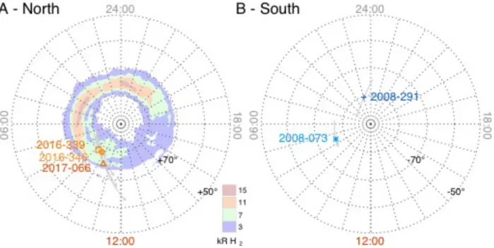
during which fSKR < fce over at least two consecutive RPWS/HFR measurements. A polar view of
the magnetic footprint of the three northern R-X mode sources identified in this study is displayed in Fig. S3A, at latitudes coincident with the average UV auroral oval (29). Fig. S3B displays a similar polar view of the two southern R-X mode sources identified in 2008 for comparison (4,11). HFR 2- and 3-antenna measurements can be inverted by goniopolarimetric (or direction-finding) inversions to retrieve the wave parameters, namely the 4 Stokes parameters S, Q, U and V and the
k-vector direction defined by 2 angular coordinates (53). 2-antenna inversions can provide 4
parameters out of 6 by assuming additional physical assumptions (for instance by fixing the source direction or neglecting the wave linear polarization). 3-antenna inversions provide the 6 wave parameters without any assumption, out of point sources. At observing latitudes beyond 30°, SKR polarization becomes strongly elliptically polarized (54), so that 3-antenna measurements are mandatory to correctly assess the wave Poynting vector (intensity S and k-vector direction) and
polarization state Q, U, V, from which the normalized linear polarization degree ; = <,+ =,
and total polarization degree > = <,+ =,+ ?, 2 are derived (31). Goniopolarimetric results
are affected by several effects described and discussed in (53,32,12). In this study, we systematically removed Radio Frequency Interferences (RFI) and applied a severe selection of 3-antenna data when studying wave polarization or direction by fixing (a) a threshold on the SNR
(conditionsimultaneously applied to the four autocorrelations of each 3-antenna measurement),
(b) a minimum total polarization T to remove aberrant or unpolarized signal and (c) a maximal
value of |zr| to remove rapidly varying signals. In such cases, we also checked that the angle
between the antenna plane and the direction of sources remained large enough to provide reliable results (53).
Fig. S4 plots dynamic spectra of S, V, L, T and of the SKR beaming angle θ over the interval 2017-066 13:00-17:00 UT, thus complementing Figs 1 and 4. SKR is generally quasi-fully polarized (Fig. S4D), with circular polarization dominant at high frequencies and low observing latitudes (Fig. S4B), while linear polarization becomes increasingly large at high latitudes and toward low frequencies (Fig. S4C) down to the SKR source region (Fig. S4A). High levels of L (and low levels
of V) measured for local waves close to fce near the SKR source region confirms previous results