HAL Id: tel-00859915
https://tel.archives-ouvertes.fr/tel-00859915
Submitted on 9 Sep 2013HAL is a multi-disciplinary open access archive for the deposit and dissemination of sci-entific research documents, whether they are pub-lished or not. The documents may come from
L’archive ouverte pluridisciplinaire HAL, est destinée au dépôt et à la diffusion de documents scientifiques de niveau recherche, publiés ou non, émanant des établissements d’enseignement et de
Modélisation des propriétés physico-chimiques des
aérosols atmosphériques à haute altitude
Aurelia Lupascu
To cite this version:
Aurelia Lupascu. Modélisation des propriétés physico-chimiques des aérosols atmosphériques à haute altitude. Sciences de la Terre. Université Blaise Pascal - Clermont-Ferrand II, 2012. Français. �NNT : 2012CLF22325�. �tel-00859915�
No d’Ordre: D.U. 2325
UNIVERSITE BLAISE PASCAL
GRADUATE SCHOOL OF FUNDAMENTAL SCIENCES
No 738
PhD. Thesis
in partial fulfillment of the requirements for the degree of
Doctor of Philosophy
Speciality: Atmospheric Physics
Submitted and presented by
Aurelia Lupascu
Modeling of physico-chemical
properties of atmospheric
aerosols at high altitude
defended the 18th of December 2012
PhD. Committee:
Chair: Dr. Nadine CHAUMERLIAC, LaMP CNRS, Clermont-Ferrand PhD. Examinators: Dr. Matthias BEEKMAN, LISA CNRS, Paris
Pr. Dr. Sabina STEFAN, University of Bucharest, Bucharest PhD. Reviewers: Dr. Edouard DEBRY, INERIS, Paris
PhD. Supervisors: Dr. Karine SELLEGRI, LaMP CNRS, Clermont-Ferrand
Acknowledgments... 7
Introduction... 9
Chapter 1. General introduction: the dynamics and the dispersion of aerosols at local scale ... 13
1.1. The atmospheric aerosols... 14
1.1.1. The sources ... 16
1.1.2. The size distribution and formation mechanism... 17
1.1.3. The aerosol transformation ... 19
1.1.4. Chemical composition ... 21
1.1.5. The deposition... 22
1.1.6. Emissions estimation ... 23
1.2. Air pollution modeling... 26
1.2.1. Modeling of atmospheric aerosols ... 28
1.2.2. Choice of Vertical Coordinate System for Air Quality Modeling... 29
1.2.3. Off-line and On-line Modeling Paradigms ... 30
1.2.4. Overview of Existing Algorithms for Aerosol Modeling ... 33
1.2.4.1. Available thermodynamic equilibrium models... 33
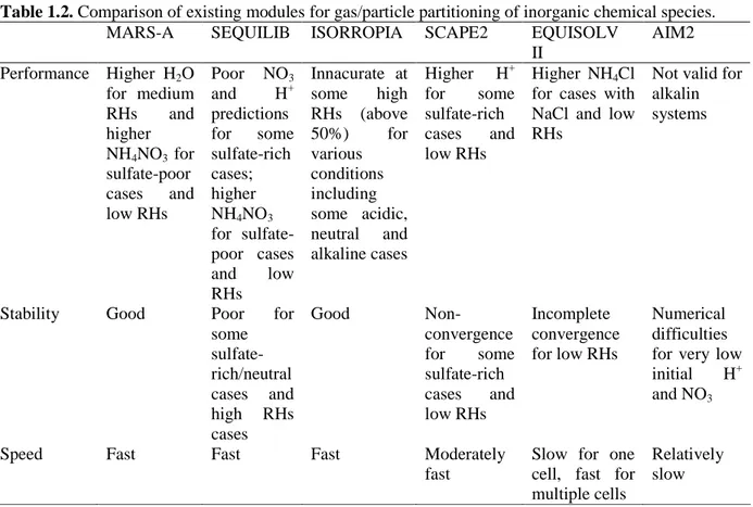
1.2.4.2. A comparison of different gas/particle models ... 36
1.2.4.3. Parameterization of the size distribution of particles... 37
1.2.4.4. Nucleation parameterizations... 38
1.2.4.5. Brownian coagulation ... 39
1.2.4.6. Condensation... 41
1.3. Conclusion ... 42
Chapter 2. The description of the meteorological model and the chemical transport model ... 43
2.1. The WRF model... 43 2.1.1. Dynamical equations... 44 2.1.2. Height coordinate... 44 2.1.3. Mass coordinate ... 46 2.1.4. Turbulent transport in PBL ... 48 2.1.5. Land-surface parameterization... 50
2.1.5.1. Thermodynamics of the LSM model ... 51
2.1.5.2. Model hydrology... 52
2.1.5.3. Snow and sea-ice model... 53
2.1.6. Soil module ... 53
2.1.7. Lateral boundary conditions ... 53
2.1.8. Nesting ... 55
2.2. The CHIMERE model ... 56
2.2.1. Model description ... 56
2.2.2. The modeling principle ... 57
2.2.3. Meteorological input data ... 57
2.2.4. The horizontal transport ... 58
2.2.5. Vertical transport and turbulent diffusion... 58
2.2.7.1. Anthropogenic emission ... 61
2.2.7.2. Biogenic emissions ... 61
2.2.7.2. Natural emissions... 62
2.2.8. Dry deposition... 63
2.2.9. Aerosols ... 64
2.2.9.1. Chemical composition and distribution of aerosols... 64
2.2.9.2. Nucleation ... 65 2.2.9.3. Coagulation ... 65 2.2.9.4. Condensation... 66 2.2.9.5. Dry deposition... 66 2.2.9.6. Wet deposition ... 67 2.3. Conclusion ... 69
Chapter 3. The influence of the emissions database on the CHIMERE simulation results... 70
3.1. Measurement sites... 71
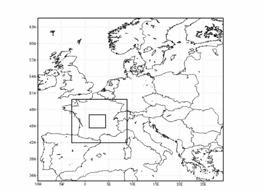
3.2. Model geometry... 74
3.2.1. WRF configuration ... 74
3.2.2. CHIMERE configuration ... 75
3.3. Simulation of the meteorological parameters ... 76
3.4. Simulation of the gaz and particulate mass concentrations in the boundary layer station 80 3.5. Simulation of the gas and particulate mass concentrations at the high altitude station... 85
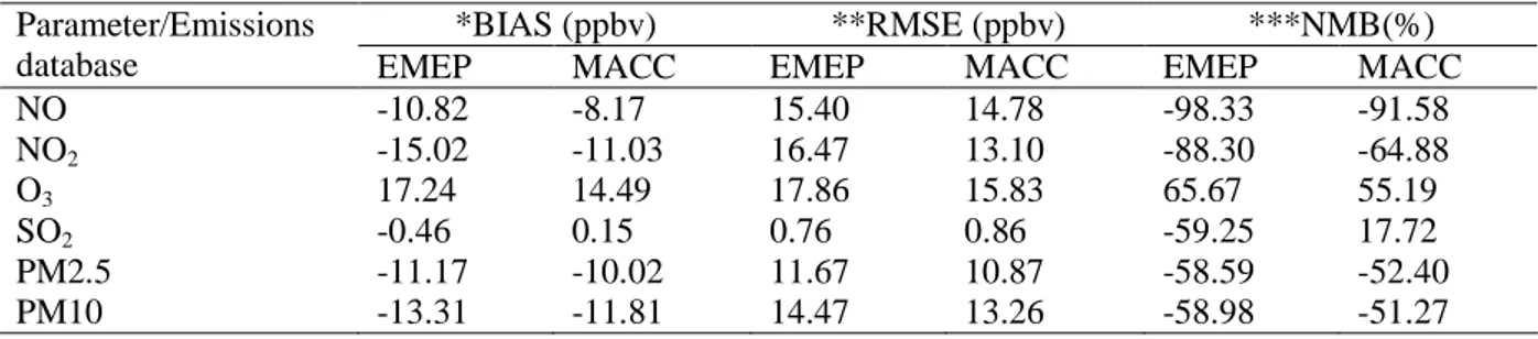
3.5.1. Gas phase components... 85
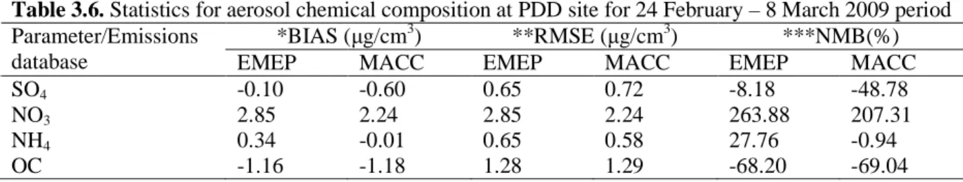
3.5.2. Aerosol phase chemical species... 91
3.6. Conclusion ... 95
Chapter 4. Model capacity to reproduce new particle formation at high altitude... 96
4.1. Introduction... 96
4.2. Description of the parameterizations ... 96
4.2.1. Kulmala’s parameterization ... 97
4.2.2. Vehkamaki’s parameterization ... 98
4.2.3. The organics parameterization ... 101
4.3. The impact of the nucleation scheme on the modeling results of CHIMERE... 102
4.3.1 Nucleation event days ... 104
4.3.1.1. March 25th, 2011 case ... 104
4.3.1.2. May 5th, 2011 case ... 109
4.3.1.3. 7-8 April 2008 case ... 115
4.3.2. Weak nucleation event days... 120
4.3.2.1. February 25th, 2009 case ... 120
4.3.2.2. March 26th, 2011 case ... 123
4.3.3. No nucleation event day... 129
4.3.3.1. March 8th, 2009 case ... 129
4.3.4. Conclusion ... 135
4.4.1. The model set-up... 136
4.4.2. Results and discussion ... 137
4.4.2.1. March 25th, 2011 case ... 137 4.4.2.2. May 5th, 2011 case ... 138 4.4.2.3. 7-8 April, 2008 case... 139 4.4.2.4. March 26th, 2011 case ... 141 4.4.2.5. February 25th, 2009 case ... 142 4.4.2.6. March 8th, 2009 case ... 143 4.4.3. Conclusion ... 144
4.5. The changes in the aerosol chemical composition due to the nucleation scheme ... 144
4.6. Is nucleation promoted at high altitude and/or promoted by force convection? ... 149
4.7. Conclusion ... 158
Summary and outlook ... 160
Acknowledgments
I am happy to take this opportunity to acknowledge and thank all those people who have helped me to reach this stage of my career. I would like to firstly thank my advisors Pr. Dr. Wolfram Wobrock and Dr. Karine Sellegri for allowing me to pursue this research and for being wonderful advisors. With their extreme patience, broad knowledge and understanding, I have learned many things about the aerosols during these three years. They led me into this exciting field, and always has been there to provide guidance and professional support. I greatly appreciate their enthusiasm and encouragement along my doctoral research.
I would like to extend my sincere thanks to my committee members: Dr. Nadine Chaumerliac, Dr. Matthias Beekmann, Pr. Dr. Sabina Stefan, and Dr. Edouard Debry for their support and interest in my research.
Many thanks to Dr. Wolfram Wobrock and Dr. Andrea Flossmann for giving me the opportunity to work in the Laboratoire de Meteorologie Physique during these three years. I am very thankful to Florence Holop and Cecile Yvetot for their assistance with the necessary paperwork.
It has been a pleasure to have worked with Cecile, Fred (they adopted me in my first day in France), Carole, Christelle, Yoann, Laurent, Evelyn, Maxime and all PhD students during my stage. Working at LaMP was very enjoyable and a very pleasant experience and all the group members treating me like one of them from the beginning, I always felt part of the group. For those who participate to the unforgettable lunch and coffee breaks very special thanks. I am grateful to Carole, Yoann, Laurent and Christelle for help me with some of the thesis arrangements.
I appreciate a lot the wonderful moments spent in France with my friends Rahimeh, Nathalie, Jean-Francois, and those who participated to the French classes.
Alphabetically, for their constant support I am grateful to Claudiu, Mirela, and Rodica.
I would specially thank Veronica for her encouragement and help during the darkness before dawn. Without her encouragement I couldn’t finish my thesis draft under the double pressure of health issues and painful writing.
Last but not the least, I would like to express my utmost thank to my family for always being on my side. Their unconditional love and support are really immeasurable and fathomless not only during my doctoral study but also throughout my whole life.
Introduction
Aerosol particles are ubiquitous in the Earth’s atmosphere. All liquid or solid particles suspended in air are defined as aerosol particles. Atmospheric aerosol particles extend over a very large range of sizes: from sub-nanometer sized clusters of molecules up to millimeter-sized dust particles. The atmospheric aerosol consists of particles from a large number of sources, both natural and anthropogenic.
Although a minor constituent of the atmosphere, the aerosol particles are linked to visibility reduction, adverse health effects and heat balance of the Earth. Particles in the atmosphere scatter and absorb solar as well as terrestrial radiation. Therefore they influence the global radiation budget directly. Besides their direct effect on the radiation budget (Bellouin et al., 2005, Yu, et al., 2006), a large fraction of the atmospheric aerosol particles acts as cloud condensation nuclei (CCN). When clouds form in the atmosphere, water condenses on the available cloud condensation nuclei. A changing in the number concentration of CCN modifies the number concentration and the size of the cloud droplets. Aerosol particles can also indirectly affect the heterogeneous chemistry of reactive greenhouse gases. While the combined global radiative forcing due to increases in major greenhouse gases (CO2, CH4 and N2O) is +2.3 Wm−2,
anthropogenic contribution to aerosol particles (primarily sulfate, organic carbon and nitrate) produce a cooling effect, with a total direct radiative forcing of −0.5 Wm−2 and an indirect cloud
albedo forcing of −0.7 Wm−2 (IPCC, 2007). Moreover, airborne particles play an important role
in the spreading of biological organisms, reproductive materials, and pathogens (pollen, bacteria, spores, viruses, etc.), and they can cause or enhance respiratory, cardiovascular, infectious, and allergic diseases (Berstein et al, 2004, Davila et al, 2007, Shiraiwa et al., 2012).
The characteristics of an aerosol population (total number concentration, size distribution, chemical composition etc.) depend on the location: urban or remote rural; continental or marine; boundary layer or higher up; as well as on the season and even the time of the day (e.g. Poschl, 2005).
Based on their source, aerosol can be divided into two groups: primary aerosols which are directly released into the atmosphere such as wave breaking and dust emissions and all type of anthropogenic emissions; and secondary aerosols which are formed in the atmosphere from the gaseous phase: precursor gases become particles by nucleation and condensation (Seinfeld and Pandis, 1998). In the latter case, chemical reactions can play an important role by turning high volatility gases into species with low vapor pressure and thus high saturation ratio, i.e. creating favorable conditions for particulate matter formation.
Nucleation is occurring when condensable vapors create stable clusters of the sub-nanometer size. The clusters grow into stable new particles with further condensational growth. This latter process is called new particle formation, and it is favored when the condensational surface represented by preexisting particles is low, while condensable precursor gases concentrations are high.
The atmospheric new particle formation processes may be relevant because the freshly formed particles can grow into sizes where they act as CCN and therefore influence cloud properties and climate (Pirjola et al., 1999, Dusek et al., 2006, Spracklen et al. 2006, Merikanto et al, 2009). Nucleation and new particle formation events have been observed in many environments.
However, information on the vertical extends of nucleation and new particle formation is rare as only few observational points exist and the measurement techniques are difficult to apply during airborne studies.
Chemical transport models can be used to ameliorate our understanding of the governing processes for aerosol formation. Modeling studies are complementary to laboratory and field campaigns for developing a complete picture of the atmospheric transformation of a species. For example, modeling work can highlight a deficiency in current understanding when the modeled and observed concentrations do not agree, and laboratory experiments can identify a new species or formation pathway to include in a model. A well developed model can then be used to diagnose how projected changes in emissions or climate may influence pollutant concentrations.
Atmospheric models constitute an important tool for simulations of transport and transformation of aerosols and gases and thus to improve our knowledge about aerosol particles primary and secondary sources of aerosol particles. The ability of chemistry-transport models (CTMs) to
accurately simulate aerosols at high altitude stations is still to be demonstrated due to reduced number of monitoring sites and difficulties to take into account the complexity of the air parcels dynamics in mountainous areas. Continuous aerosol measurements have mostly been carried out at low altitudes. This is reasonable because the stations are easier to be built and operated there. However, low-altitude measurements are easily affected by local aerosol sources and small-scale meteorological patterns in boundary layer. Regional and large-scale concentration levels of aerosol particles can therefore be observed more reliably in measurements conducted at high altitudes. Observations from high-altitude stations have a special significance as the aerosols in this region are far from potential sources and are more representative of background conditions and a greater spatial extent (Asmi, 2011).
The goal of this thesis is to investigate the capability of the regional air-quality model CHIMERE to reproduce the mass and number concentrations and temporal evolution of the aerosols particles at high altitudes (as for example Puy de Dome research station), and in particular, evaluate its capacity to simulate the formation of new particles due to nucleation. Specifically, this thesis aims to address the following questions:
-What is the impact of a fine resolution topographical database on the accuracy of simulation of dynamical parameters at high altitude?
-What is the impact of the use of different emissions databases in the accuracy of gas-phase and aerosol concentration predictions?
-What is the most adequate nucleation parameterization scheme for simulating new particle formation at high altitude?
-What is the influence of the choice of the primary particle size distribution on the prediction of new particle formation?
The observed data used to compare with the modeling results are from the Puy de Dome research station (45º 46' 15'' N; 2º 57' 50'' E, 1465 m a.s.l.). This station provides continuous measurements of the aerosol particle size distribution, aerosol hygroscopicity, aerosol particle nucleation in the nano-meter range. The work of Boulon et al., 2011 presents an analysis of the
the surface station Opme (660 m asl) located around 12 km South-Easth of the Puy de Dome station. They showed that the frequency of nucleation events was higher at Puy de Dome site (97.5% of events detected) in comparison with lower station of Opme (56% of events detected) leading to the conclusion that the nucleation process is clearly enhanced at the high altitude station and the new particle formation process usually occurs in elevated altitudes.
Additionally, during intensive field campaigns, on-line chemical analysis of the aerosol is available with high time resolution. We propose here to confront the regional air-quality model CHIMERE coupled with the meteorological model WRF both with high altitude measurements performed at the Puy de Dome station and with ground based measurements made inside the urban boundary layer of Clermont-Ferrand.
This thesis is structured as follows: the first chapter will provide an overview of the relevant aspects of aerosol in the atmosphere and previous modeling approaches. Chapter 2 describes our modeling system and introduces the various parts of the computer models we used. Chapter 3 presents the evaluation of both the meteorological model and the air quality models using for the meteorological model two different topographical inputs and for the air quality model two different emission databases. Results of the simulations using different nucleation schemes are presented and discussed in chapter 4. Three nucleation parameterizations are tested using the CHIMERE model. Weak, moderate, and strong nucleation events of aerosol particles together with days without nucleation from observation performed at Puy de Dome research station are selected for the evaluation. The ability of the different theories to reproduce the occurrence or lack of a nucleation event is evaluated. Subsequently, these results are summarized and implications of our findings discussed. A brief outlook on the direction of future research is given in the last chapter.
Chapter 1. General
introduction: the dynamics and
the dispersion of aerosols at
local scale
This chapter is dedicated to presenting fundamental information on aerosols and their properties, and the description of the general principles of numerical modeling of the particles. First, the various constituents of aerosol and their microphysical properties are described. In the last section of this introductory chapter, we give a summary of current knowledge and major advances in aerosol modeling. Different approaches for the inclusion of particles in the models are described based on a literature review.
Aerosols play a key role in many fields and on many scales of atmospheric and climate science, ranging from the nanometer scale of molecular interactions and chemical reactions to the global scale of the climate system. The recently published Fourth Assessment Report (AR4) of the United Nations Intergovernmental Panel on Climate Change (IPCC) states that the full range of processes leading to modification of cloud properties by aerosols is not well understood and the magnitudes of associated indirect radiative effects are poorly determined (Solomon et al., 2007). The tropospheric aerosol consists of water, inorganic acids and salts, and many different organic compounds originating from natural and anthropogenic processes. Numerous individual organic compounds present in ambient aerosol samples have been identified (e.g. Mazurek et al., 1997; Pio et al., 2001; Tsapakis et al., 2002). These compounds consist mostly of different alkanes, acids, alcohols, aldehydes, ketones, nitrates and aromatic hydrocarbons. Thus, the tropospheric aerosol is, from a physicochemical point of view, an organic-inorganic mixture. Figure 1.1 shows a selection of important atmospheric topics and effects related to the composition and non-ideal thermodynamics of mixed organic-inorganic aerosol particles.
Figure 1.1. The thermodynamics of mixed aerosol and related effects
Tropospheric aerosols, especially the very fine particles originating from anthropogenic activities, have an impact on air quality and human health. In addition, scattering and absorption of solar and terrestrial radiation influence the visibility and the earth's radiative budget.
Numerical models of meteorology and air quality can play a role in characterizing the concentration and properties of aerosol. They are also useful tools to explore control strategies, provide short-term forecasts, test our understanding of the science, and explore new theories about air pollution science.
1.1. The atmospheric aerosols
The atmospheric aerosols are particles in suspension in the air. They represent the condensed phase in liquid and solid form. Many classifications are used to describe the aerosols phase: in function of their origin (natural or anthropogenic), of their nature (inorganic or organic), of their size (the number distribution). The aerosols size varies from one nanometer to a few tens of microns. The aerosols with superior size are not generally considered as particles in suspension because they can sediment under gravitational effect. The inferior limit corresponds to the smaller condensation nuclei measured until now. If more than 90% of particles in suspension have a diameter less than 0.1 µm, the mass majority is composed of particles having a superior diameter.
The term “atmospheric aerosols” encompasses a wide range of particle types having different compositions, sizes, shapes and optical properties. Aerosol loading, or amount in the atmosphere,
is usually quantified by mass concentration or by an optical measure, aerosol optical depth (AOD). Usually numerical models and in situ observations use mass concentration as the primary measure of aerosol loading (Remer et al., 2009).
Aerosols interact both directly and indirectly with the Earth's radiation budget and climate. As a direct effect, the aerosols scatter sunlight directly back into space. As an indirect effect, aerosols in the lower atmosphere can modify the size of cloud particles, changing how the clouds reflect and absorb sunlight, thereby affecting the Earth's energy budget.
Aerosols also can act as sites for chemical reactions to take place (heterogeneous chemistry). The most significant of these reactions are those that lead to the destruction of stratospheric ozone. During winter in the polar region, aerosols grow to form polar stratospheric clouds. The large surface areas of these cloud particles provide sites for chemical reactions to take place. These reactions lead to the formation of large amounts of reactive chlorine and, ultimately, to the destruction of ozone in the stratosphere. Evidence now exists that shows similar changes in stratospheric ozone concentrations occur after major volcanic eruptions, like Mt. Pinatubo in
1991, where tons of volcanic aerosols are blown into the atmosphere
(http://www.nasa.gov/centers/langley/news/factsheets/Aerosols.html).
The radiative effects of aerosols affect the climate opposite to that of increasing concentrations of greenhouse gas emissions (which contribute to the global warming). The lifetime of aerosols, however, is much shorter, in general, than that of greenhouse gas emissions. Quantitatively, on a global scale, the radiative impacts of particles do not compensate the radiative impact of greenhouse gas emissions. However, locally, the concentrations of aerosols can be very important. The radiative effects can then have important consequences (IPCC, 2007). By increasing aerosol and cloud optical depth, anthropogenic emissions of aerosols and their precursors contribute to a reduction of solar radiation at the surface. As such, worsening air quality contributes to regional aerosol effects. The decline in solar radiation from 1961 to 1990 affects the partitioning between direct and diffuse solar radiation: Liepert and Tegen (2002) concluded that over Germany, both aerosol absorption and scattering must have declined from 1975 to 1990 in order to explain the simultaneously weakened aerosol forcing and increased direct/diffuse solar radiation ratio. The direct/diffuse solar radiation ratio over the USA also increased from 1975 to 1990, likely due to increases in absorbing aerosols. Increasing aerosol
fraction of diffuse radiation at the surface, which results in larger carbon assimilation into vegetation (and therefore greater transpiration) without a substantial reduction in the total surface solar radiation (Niyogi et al., 2004, IPCC, 2007).
The aerosols can significantly alter the chemical composition of the atmosphere (Faust, 2004). They can absorb semi-volatile species thus changing the kinetic equilibrium. Also the heterogeneous reactions can occur on the surface of aerosols. The particles then behave as a catalyst for the chemical reactions that affect the gas phase.
Finally, aerosols can have significant health impacts. The fine and ultrafine particles enter the respiratory system. Aerosols carry various chemical species, particularly organic species, which can cause inflammatory and/or allergenic reactions. The aerosols are, also correlated to certain cardiovascular diseases. Suspected are especially the ultrafine particles which can cross the respiratory mucosa and to be responsible for systemic effects, including blood coagulation and cardiovascular effects. These effects appear to be strongly dependent on the diameter of the particles and their chemical composition (WHO, 2000).
One of the greatest challenges in studying aerosol impact is the immense diversity, not only in particle size, composition, and origin, but also in spatial and temporal distribution. For most aerosols, whose primary source is emissions near the surface, concentrations are greatest in the atmospheric boundary layer, decreasing with altitude in the free troposphere. However, smoke from wildfires and volcanic effluent can be injected above the boundary layer, after injection, any type of aerosol can be lofted to higher elevation, this can extend their atmospheric lifetimes, increasing their impact spatially and climatically.
1.1.1. The sources
Atmospheric particles are produced by two distinctly different mechanisms: particulate emissions produce primary particles spanning a wide range of sizes, and gas-to-particle conversion creates nanometer-sized particles by atmospheric nucleation, or new material on all sizes by condensation, both process being called secondary production. These production mechanisms differ greatly in their spatial and temporal variations and the factors that control these variations. For example, particulate emissions occur almost universally close to the ground whereas nucleation occurs in the boundary layer (Kulmala et al., 2004) and in the upper
troposphere (Twohy et al., 2002; Benson et al., 2008). The increased aerosol concentrations are largely due to secondary particle production, i.e. homogeneous nucleation and subsequent growth from vapors.
An important part of the atmospheric aerosols mass have a natural primary origin. As an example of primary sources we can mention mainly the erosion of dust under the action of the wind, the formation of marine aerosols released by the burst at the surface of an ocean of bubbles air forms at the breaking waves, the volcanic eruptions or the biogenic aerosols made by the various activities of the planet.
The anthropogenic aerosols come principally from the road and the air traffic, and various industrial activities. However, we could also note all combustion processes such as fires, which had in the past disastrous health consequences, or the cigarettes smoke. The emission of volatile organic compounds (VOCs) of anthropogenic origin is a source of secondary aerosols. Indeed, these VOCs can be oxidized in the atmosphere giving rise to compounds whose saturated vapor pressure is low enough to form secondary aerosols by the transformation process gas/particle.
1.1.2. The size distribution and formation
mechanism
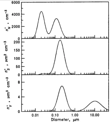
The size of atmospheric particles varies from one nanometer to a few tens of microns and has an influence on their lifetime in the atmosphere that can vary from a couple of hours to several weeks. Moreover, the optical properties of aerosols, together with their effect on environment and health vary considerably as a size function. The size distribution can be represented in number, mass, volume or surface. The aerosol distribution is controlled by a complex system of physical processes. The experimental characterization of the spectral distribution proposed by Whitby (1976) highlights three principal modes (see Figure 1.2):
- the nucleation mode containing ultrafine particles having the diameter less than 0.1 micrometer, formed mainly by condensation of vapors during combustion processes at high temperatures or by homogeneous nucleation during cooling. These particles can then grow by coagulation between themselves or with larger particles and thus passing into the higher mode, which is the main loss in this mode. Although the largest number of airborne particles appear in the
nucleation mode, these particles give a small contribution to the total mass of particles because of their very small size.
- the accumulation mode contains particles with a diameter between 0.1 and 2 microns resulting from the coagulation of nucleation mode particles and condensation of vapors on existing particles whose size increases while they are in the range. This mode is a major contributor to the surface and the total mass of aerosols in the atmosphere. The accumulation mode is so called because the atmospheric removal processes are less efficient in this size range. These fine particles can remain in the atmosphere for days or weeks. Dry and wet depositions (precipitation scavenging) are the main processes by which these particles are eventually removed from the atmosphere.
- the coarse mode contains particles with a diameter greater than 2 microns, generally formed by mechanical processes such as wind erosion, breaking ocean waves, grinding operations in the industry, etc. These particles are efficiently removed by settling under the action of gravity. Their life is short, from several hours to several days. They have a small contribution to the number concentration of particles, but much to their total mass.
Figure 1.2. Typical remote continental aerosol number, surface and volume distributions (Reproduced
1.1.3. The aerosol transformation
Once suspended in the atmosphere, aerosols can undergo transformations (changes in size and/or chemical composition) under the action of microphysical processes:
• the condensation (evaporation) of gas molecules of gas from the surface of the aerosol.
• the coagulation of aerosols between them.
• the nucleation: from a thermodynamically unstable phase, liquid or solid fragments of a
new phase more stable are formed.
The ensemble of these processes is described by the models of aerosols dynamics.
The aerosol particle size distribution and its temporal and spatial variability is a fundamental aerosol property, especially regarding CCN activity. Nucleation is one of the key process controlling particles number distributions (Merikanto et al., 2009). Model estimates suggest that new particle formation can contribute up to 40% of the CCN at the boundary layer, and 90% in the remote troposphere (Pierce and Adams, 2007).
Pure sulfuric acid (H2SO4) has a low vapor pressure at atmospheric temperatures (Ayers et al.,
1980). The H2SO4 vapor pressure is reduced further in the presence of water (Marti et al, 1997)
due to the large mixing enthalpy that is freed when the two substances are mixed. When H2SO4
is produced from sulfur dioxide (SO2) in the gas phase, it is therefore easily super-saturated and
the gaseous H2SO4 starts to condense. Water vapor is omnipresent in the atmosphere and
therefore a condensation of H2SO4 and H2O is always occurring. If the gaseous H2SO4 molecules
do not encounter pre-existing (aerosol) surfaces to condense on before colliding with other H2SO4 and H2O molecules, they may cluster with the other molecules. If these clusters continue
to grow and overcome the nucleation barrier, then new, thermodynamically stable aerosol particles are formed from the gas phase. This is termed binary homogeneous nucleation: binary
for the two substances H2SO4 and H2O that nucleate and homogeneous because no other catalyst
like a foreign surface is involved in the formation.
Nucleation was observed at a range of atmospheric and meteorological conditions. Many open questions remain about the details of the nucleation mechanism and about the nucleating agents. The nucleation and subsequent growth processes influence the total particle number, the particle
Climatic effects, like the indirect aerosol effects, are potentially influenced by the number of nucleation mode particles growing to sizes at which they can become active cloud condensation nuclei (Spracklen et al., 2006, Pirjola et al., 2004). Sulfur dioxide is considered the most important precursor gas for atmospheric nucleation particles. It is emitted into the atmosphere mostly by anthropogenic sources such as combustion of sulfur-containing fossil fuels (Stern, 2005). Therefore, aerosol nucleation in the atmosphere would be expected to be enhanced by anthropogenic activities. On the other hand, the pre-existing aerosol that can take up gaseous sulfuric acid and thereby suppressing nucleation is increased as well by anthropogenic sources. Several nucleation mechanisms have been discussed to occur in the atmosphere. The binary nucleation of sulfuric acid and water (Noppel, et al., 2002, Vehkamaki et al., 2002, Yu, 2006,
Hanson, Lovejoy, 2006), the ternary nucleation of H2SO4, H2O, and ammonia (NH3) (Coffman et
al., 1995, Weber et al., 1996, Korhonen et al, 1999, Yu, 2006), ion-induced nucleation (Yu, Turco, 2001, Laakso et al., 2002, Eichkorn et al. 2002, Lee, et al., 2004, Lovejoy et al., 2004, Kazil, Lovejoy, 2004) and reactive nucleation involving sulfuric acid and organic acids (R.H. Zhang et al., 2004, Metzger et al., 2010) are most prominent.
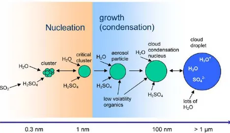
The schematics of an atmospheric nucleation process of H2SO4 and H2O with subsequent growth
involving also organics is illustrated in Fig. 1.3. The particles eventually may grow large enough to act as cloud condensation nuclei.
Figure 1.3. Schematic representations of the nucleation and subsequent growth process for atmospheric
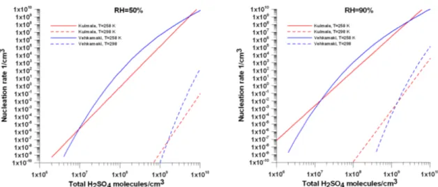
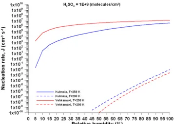
Parameterized equations of the nucleation rates, size of the critical cluster and critical cluster composition as a function of the gas-phase concentration of the involved chemical species and as
a function of temperature have been derived for the binary H2SO4/H2O system (Kulmala et al.,
1998, Vehkamaki et al., 2002), the ternary H2SO4/H2O/NH3 system (Napari et al., 2002b), the
ion-induced nucleation of the H2SO4/H2O system (Modgil et al, 2005) as well as for organics
nucleation (Metzger et al., 2010).
1.1.4. Chemical composition
We distinguish between inorganic aerosols and organic aerosols. The major inorganic species simulated in the aerosol models include sulfates, nitrates, chlorates, ammonia and sodium. Organic species are less well known (especially their activity). For this reason the modeled species are generally used to simulate the organic phase with the method of allocation between phases simplified. Finally, inert species such as mineral dust and elemental carbon also contribute significantly to the aerosol mass.
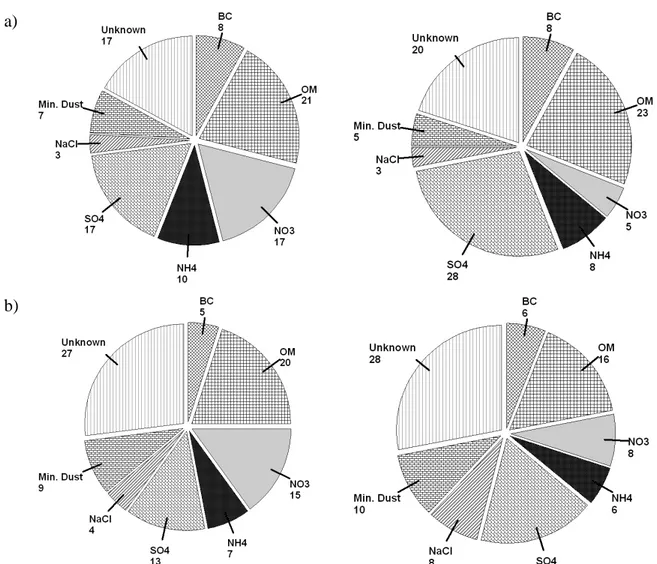
The study made by Putaud et al. (2004) give a detailed chemical characterization of the aerosol for various European sites (urban, rural, traffic). A fairly homogeneous composition of PM2.5 and PM10 were observed on different urban sites. As shown in Fig. 1.4, the urban aerosol (PM2.5 and PM10) is composed from 5 to 10% of black carbon, 20% organic matter, from 35 to 45% inorganic material and 5 to 10% mineral dust. This predominance of organic matter and the inorganic fraction in the secondary composition the aerosol attests the importance of the processes of secondary particulate formation and transport over long distances. The coarse fraction of the aerosol is mainly composed of mineral dust (> 20%) and salt (10%). The unidentified fraction ("unknown") of the aerosol is between 17 and 45% of the total mass, which illustrates the difficulty of measuring the composition of the particles, due to the variety of its constituents and limits of measuring instruments. The difference between urban and rural sites lies mainly in the relative contribution of largest nitrate and ammonium in urban areas, and sulfates in rural areas.
a)
b)
Figure 1.4. The average composition of PM2.5 (a) and PM10 (b) observed in several European stations
(urban-left panel and rural-right panel). Adapted from (Putaud et al. 2004)
1.1.5. The deposition
Once suspended in the atmosphere, the aerosols have a limited lifetime before deposition or transformation. The average lifetime of aerosols ranges from few days to one week. However, the lifetime depends on aerosols size and also of its environment.
There is principally two deposition phenomenon:
− dry deposition which depends essentially on the soil rugosity that characterize the capacity to capture the suspended particles;
1.1.6. Emissions estimation
Aerosols have various sources from both natural and anthropogenic processes. Natural emissions include wind-blown mineral dust, aerosol and precursor gases from volcanic eruptions, natural wild fires, vegetation, and oceans. Anthropogenic sources include emissions from fossil fuel and biofuel combustion, industrial processes, agriculture practices, and human-induced biomass burning.
Following earlier attempts to quantify man-made primary emissions of aerosols (Turco et al., 1983; Penner et al., 1993), a systematic work was undertaken in the late 1990s to calculate emissions of black carbon (BC) and organic carbon (OC), using fuel-use data and measured emission factors (Liousse et al., 1996; Cooke and Wilson, 1996; Cooke et al., 1999). The work was extended in greater detail and with improved attention to source-specific emission factors in Bond et al. (2004), who provides global inventories of BC and OC for the year 1996, with regional and source-category discrimination that includes contributions from industrial, transportation, residential solid-fuel combustion, vegetation and open biomass burning (forest fires, agricultural waste burning, etc.), and diesel vehicles.
Emissions from natural sources—which include wind-blown mineral dust, wildfires, sea salt, and volcanic eruptions—are less well quantified, mainly because of the difficulties of measuring emission rates in the field and the unpredictable nature of the events. However, dust emission schemes that have been developed and used in the regional models range from simple type schemes, in which the vertical dust flux depends on a prescribed erodible surface fraction and fixed threshold friction velocity (Gillette and Passi, 1998; Uno et al., 2001) to advanced schemes, in which the surface characteristics are taken into account explicitly in the parameterizations of the threshold friction velocity, and horizontal and vertical fluxes (Marticorena and Bergametti, 1995; Shao et al., 1996; Shao, 2004). Every dust emission scheme adopts different parameterizations for the wind erosion mechanism and the influence of input parameters is different, thus the scattering of simulation results is yielded.
Sea salt aerosol (SSA) often dominates the mass concentration of marine aerosol, especially at locations remote from anthropogenic or other continental sources, and SSA is one of the dominant aerosols globally (along with mineral dust) in terms of mass emitted into the
the size-distributed number production flux times the volume per particle times the mass of sea salt per unit volume of seawater) with current chemical transport models and global climate models, using various parameterizations of the sea spray source function (SSSF), range over
nearly 2 orders of magnitude, from 0.02 to 1 × 10¹⁴ kg yr−1 (Textor et al., 2006). Much of this
variation is due to the different dependences on wind speed and to the upper size limit of the particles included.
Aerosols can be produced from atmospheric trace gases via chemical reactions, and those aerosols are called secondary aerosols, as distinct from primary aerosols that are directly emitted to the atmosphere as aerosol particles.
For example, most sulfate and nitrate aerosols are secondary aerosols that are formed from their precursor gases, sulfur dioxide (SO2) and nitrogen oxides (NO and NO2, collectively called
NOx), respectively.
The formation of ammonium nitrate aerosol depends on the thermodynamic state of its precursor and depends strongly on the environmental conditions. Gaseous ammonia and nitric acid react in
the atmosphere to form aerosol ammonium nitrate, NH4NO3.
NH3(g) + HNO3(g) ↔ NH4NO3(s) (1.1)
Ammonium nitrate is formed in areas characterized by high ammonia and nitric acid conditions and low sulfate conditions. Depending on the ambient relative humidity (RH), ammonium nitrate may exist as a solid or as an aqueous solution of NH4 and NO3. Equilibrium concentrations of
gaseous NH3 and HNO3, and the resulting concentration of NH4NO3 is calculated by
thermodynamical principals, requiring the ambient RH and temperature. At low temperatures the equilibrium of the system shifts towards the aerosol phase. At low RH conditions NH4NO3 is
solid, and at RH conditions above the deliquescence, NH4NO3 will be found in the aqueous state.
NH3(g) + HNO3(g)↔ NH4+ NO3. (1.2)
For a given temperature the solution of the equilibrium equation requires the calculation of the corresponding molarities. These concentrations depend not only on the aerosol nitrate and ammonium but also on the amount of water in the aerosol phase. Therefore, calculations of the
aerosol solution composition require estimation of the aerosol water content. The presence of water allows NH4NO3 to dissolve in the liquid aerosol particles and increases its aerosol
concentration. Ammonium and nitrate will exist in the aerosol phase only if there is enough ammonia and nitric acid present to saturate the gas phase.
Sulfuric acid plays an important role in nitrate aerosol formation. Sulfuric acid possesses an
extremely low vapor pressure. Furthermore (NH4)2SO4 is the preferred form of sulfate, so each
mole of sulfate will remove 2 moles of ammonia from the gas phase.
NH3 + H2SO4(g)↔ (NH4)HSO4 (1.3)
NH3 + (NH4)H2SO4(g)↔ (NH4)2SO4 (1.4)
Therefore two regimes are important for nitrate formation: the rich and the ammonia-poor case.
Heterogeneous reactions of gaseous species with coarse aerosol species, like mineral dust and
sea salt particles, have an important impact on NH4NO3 formation. Once HNO3 is formed, it is
most likely captured by coarse mode sea-salt and dust particles, leading to a depletion of aerosol nitrate in the fine mode. During the night when ammonia is present in excess, ammonium nitrate can be formed; however, since this salt is thermodynamically not stable, it can evaporate during the day whereby the aerosol precursor gases NH3 and HNO3 are likely to condense on
preexisting and larger aerosol particles (Wexler and Seinfeld, 1990).
Those sources have been studied for many years and are relatively well known. By contrast, the sources of secondary organic aerosols (SOA) are poorly understood, including emissions of their precursor gases (called volatile organic compounds, VOC) from both natural and anthropogenic sources and the atmospheric production processes.
Globally, sea salt and mineral dust dominate the total aerosol mass emissions because of the large source areas and/or large particle sizes.
However, sea salt and dust also have shorter atmospheric lifetimes because of their large particle size, and are radiatively less active than aerosols with small particle size, such as sulfate, nitrate, BC, and particulate organic matter (POM, which includes both carbon and non-carbon mass in the organic aerosol), most of which are anthropogenic in origin.
1.2. Air pollution modeling
Air pollution modeling is a numerical tool used to describe the causal relationship between emissions, meteorology, atmospheric concentrations, deposition, and other factors. Air pollution measurements give important, quantitative information about ambient concentrations and deposition, but they can only describe air quality at specific locations and times, without giving clear guidance on the identification of the causes of the air quality problem. Air pollution modeling, instead, can give a more complete deterministic description of the air quality problem, including an analysis of factors and causes (emission sources, meteorological processes, and physical and chemical changes), and some guidance on the implementation of mitigation measures.
Air pollution models play an important role in science, because of their capability to assess the relative importance of the relevant processes. Air pollution modeling is the only method which quantifies the deterministic relationship between emissions and concentrations/depositions, including the consequences of past and future scenarios and the determination of the effectiveness of abatement strategies. This makes air pollution models indispensable in regulatory, research, and forensic applications.
The concentrations of substances in the atmosphere are determined by: 1) transport, 2) diffusion, 3) chemical transformation, and 4) deposition on the ground. Transport phenomena, characterized by the mean velocity of the fluid, have been measured and studied for centuries. For example, the average wind has been studied by man for sailing purposes. The study of diffusion (turbulent motion) is more recent.
Among the first articles that mention turbulence in the atmosphere, are those by Taylor (1915, 1921).
One of the first challenges in the history of air pollution modeling (e.g., Sutton, 1932, Bosanquet, 1936) was the understanding of the diffusion properties of plumes emitted from large industrial stacks. For this purpose, a very successful, yet simple model was developed – the Gaussian Plume Model. This model was applied for the main purpose of calculating the maximum ground level impact of plumes and the distance of maximum impact from the source. The model was formulated by determining experimentally the horizontal and vertical spread of the plume, measured by the standard deviation of the plume’s spatial concentration distribution.
Experiments provided the geometrical description of the plume by plotting the standard deviation of its concentration distribution, in both the vertical and horizontal direction, as a function of the atmospheric stability and downwind distance from the source. Atmospheric stability is a parameter that characterizes the turbulent status of the atmosphere.
In the 1960s, the studies concerning dispersion from a point source continued and were broadening in scope. Major studies were performed by Hogstrom (1964), Turner (1964), Briggs (1965) (the developer of the well-known plume-rise formulas), Moore (1967), Klug (1968). The use and application of the Gaussian plume model spread over the whole globe, and became a standard technique in every industrial country to calculate the stack height required for permits. The Gaussian plume model concept was soon applied also to line and area-sources. Gradually, the importance of the mixing height was realized (Holzworth, 1967, Deardorff, 1975) and its major influence on the magnitude of ground level concentrations. To include the effects of the mixing height, multiple reflections terms were added to the Gaussian Plume model (e.g., Yamartino, 1977).
Shortly after 1970, scientists began to realize that air pollution was not only a local phenomenon. It became clear - firstly in Europe - that the SO2 and NOx emissions from tall stacks could lead to
acidification at large distances from the sources. It also became clear - firstly in the US - that ozone was a problem in urbanized and industrialized areas. And so it was obvious that these situations could not be tackled by simple Gaussian-plume type modeling.
Two different modeling approaches were followed, Lagrangian modeling and Eulerian modeling. In Lagrangian modeling, an air parcel (or “puff”) is followed along a trajectory, and is assumed to keep its identity during its path. In Eulerian modeling, the area under investigation is divided into grid cells, both in vertical and horizontal directions.
Lagrangian modeling, directed at the description of long-range transport of sulfur, began with studies by Rohde (1972, 1974), Eliassen (1975) and Fisher (1975). The work by Eliassen was the start for the well-known EMEP-trajectory model which has been used over the years to calculate air pollution of acidifying species and later, photo-oxidants. Lagrangian modeling is often used to cover longer periods of time, up to years.
Eulerian modeling began with studies by Reynolds (1973) for ozone in urbanized areas, with Shir and Shieh (1974) for SO2 in urban areas, and Egan (1976) and Carmichael (1979) for
known Urban Airshed Model-UAM originated for photochemical simulations. Eulerian modeling, in these years, was used only for specific episodes of a few days.
So in general, Lagrangian modeling was mostly performed in Europe, over large distances and longer time-periods, and focused primarily on SO2. Eulerian grid modeling was predominantly
applied in the US, over urban areas and restricted to episodic conditions, and focused primarily
on O3. Also hybrid approaches were studied, as well as particle-in-cell methods (Sklarew et al.,
1971). Early papers on both Eulerian and Lagrangian modeling are by Friedlander and Seinfeld (1969), Eschenroeder and Martinez (1970) and Liu and Seinfeld (1974).
A comprehensive overview of long-range transport modeling in the seventies was presented by Johnson (1980).
The next, obvious step in scale is global modeling of the earth’s troposphere. The first global models were 2-D models, in which the global troposphere was averaged in the longitudinal direction (Isaksen, 1978). The first, 3-D global models were developed by Peters (1979) (see also Zimmermann, 1988).
It can be stated that, since approximately 1980, the basic modeling concepts and tools were available to the scientific community. Developments after 1980 concerned the fine-tuning of these basic concepts.
Photochemical air quality models have become widely recognized and routinely utilized tools for regulatory analysis and attainment demonstrations by assessing the effectiveness of control strategies. These photochemical models are large-scale air quality models that simulate the changes of pollutant concentrations in the atmosphere using a set of mathematical equations characterizing the chemical and physical processes in the atmosphere. These models are applied at multiple spatial scales from local, regional, national, and global.
1.2.1. Modeling of atmospheric aerosols
The aerosols modeling capability has developed rapidly in the past decade. In the late 1990s, there were only a few models that were able to simulate one or two aerosols components, but now there are a few dozen models that simulate a comprehensive suite of aerosols in the atmosphere. As introduced before, aerosols consist of a variety of species, including dust, sea salt, sulfate, nitrate, and carbonaceous aerosols (black and organic carbon) produced from natural
and man-made sources with a wide range of physical properties. Because of the complexity of the processes and composition, and highly inhomogeneous distribution of aerosols, accurately modeling atmospheric aerosols and their effects remains a challenge. Models have to take into account not only the aerosol and precursor emissions, but also the chemical transformation, transport, and removal processes (e.g. dry and wet depositions) to simulate the aerosol mass concentrations. Furthermore, aerosol particle size can grow in the atmosphere because the ambient water vapor can condense on the aerosol particles. This “swelling” process, called hygroscopic growth, is most commonly parameterized in the models as a function of relative humidity. Modeling plays a key role for quantitatively integrating knowledge and for evaluating our understanding of physical and chemical processes in the atmosphere. The main goal of aerosol modeling is to establish a detailed description of the aerosol particle concentrations and their composition and size distribution. This requires advanced modeling techniques and innovation as well as reliable validation data of particle characteristics. The aerosol modules implemented in a chemistry transport models generally take into account gas-to-particle conversion and aerosol dynamics and enable simulation of the complete aerosol number/mass/composition distribution.
1.2.2. Choice of Vertical Coordinate System for Air
Quality Modeling
Many different types of vertical coordinates have been used for various meteorological simulations. For example, the geometric height is used to study boundary layer phenomenon because of its obvious advantage of relating near surface measurements with modeled results. Pressure coordinates are natural choices for atmospheric studies because many upper atmospheric measurements are made on pressure surfaces. Because most radiosonde measurements are based on hydrostatic pressure, one may prefer use of the pressure coordinate to study cloud dynamics. This idea of using the most appropriate vertical coordinate for describing a physical process is referred to as a generic coordinate concept (Byun et al., 1995). Several different generic coordinates can be used in a CTM for describing different atmospheric processes while the underlying model structure should be based on a specific coordinate
Byun (1999a) discusses key science issues related to using a particular vertical coordinate for air quality simulations. They include a governing set of equations for atmospheric dynamics and thermodynamics, the vertical component of the Jacobian (metric tensor associated with the vertical coordinate transformation), the form of continuity equation for air, the height of a model layer (expressed in terms of geopotential height), and other special characteristics of a vertical coordinate for either hydrostatic or non-hydrostatic atmosphere applications.
Not only the assumptions on atmospheric dynamics, but also the choice of coordinate can affect the characteristics of atmospheric simulations. For the time-independent vertical coordinates (z, p, sigma-z, sigma-p), the vertical Jacobians are also time-independent. Especially with the hydrostatic assumption, one can obtain a diagnostic equation for the vertical velocity component which includes sound-waves together with meteorological signals. Further assumptions on flow characteristics, such as anelastic approximation, provide a simpler diagnostic equation for the non-solenoidal air flow. For such cases, with or without the anelastic approximation, one can maintain trace species mass conservation in a CTM by using the vertical velocity field estimated from the diagnostic relation. This diagnostic works whether the horizontal wind components, temperature, and density field data are directly provided from a meteorological model or interpolated from hourly data at the transport time step. This suggests that the mass error can be estimated with the diagnostic relations that originate from one of the governing equations of the preprocessor meteorological models. For a non-hydrostatic atmosphere, which does not have a special diagnostic relation for time independent coordinate, one should rely on methods to account for the mass consistency errors.
1.2.3. Off-line and On-line Modeling Paradigms
Air quality models are run many times to understand the effects of emissions control strategies on the pollutant concentrations using the same meteorological data. A non-coupled prognostic model can provide adequate meteorological data needed for such operational use. This is the so-called off-line mode air quality simulation. However, a successful air quality simulation requires that the key parameters in meteorological data be consistent. For example, to ensure the mass conservation of trace species, the density and velocity component should satisfy the continuity equation accurately. Details of this issue will be discussed below.
Dynamic and thermodynamic descriptions of operational meteorological models should be self-consistent, and necessary meteorological parameters are readily available at the finite time steps needed for the air quality process modules during the numerical integration. This is the so-called on-line mode air quality simulation. There have been a few successful examples of integrating meteorology and atmospheric chemistry algorithms into a single computer program (e.g., Vogel et al., 1995, Arteta, 2005). For certain research purposes, such as studying two-way interactions of radiation processes, the line modeling approach is needed. However, the conventional on-line modeling approach, where chemistry-transport code is imbedded in one system, exhibits many operational difficulties. For example, in addition to tremendously increasing the computer resource requirements, differences in model dynamics and code structures hinder development and maintenance of a fully coupled meteorological/chemical/emissions modeling system for use in routine air quality management.
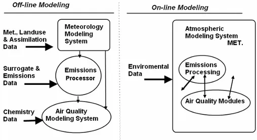
Figure 1.5 shows structures of the on-line and off-line air quality modeling systems, respectively, commonly used at present time.
Figure1.5. The structure of current on-line and off-line air quality models
Table 1.1 compares a few characteristics of on-line and off-line modeling paradigms (Byun, 1999b). Each method has associated pros and cons. However, to accomplish the goals of multiscale on-line/off-line modeling with one system, a full adaptation of the one-atmosphere
• Development of the fully coupled chemistry-transport model to a meteorological modeling system requires a fundamental rethinking of the atmospheric modeling approach in general.
Some of the suggested requirements for a next generation mesoscale meteorological model that can be used as a host of the on-line/off-line modeling paradigms are:
• Scalable dynamics and thermodynamics: Use fully compressible form of governing set of
equations and a flexible coordinate system that can deal with multiscale dynamics.
• Unified governing set of equations: Not only the weather forecasting, dynamics and
thermodynamics research but also the air quality studies should rely on the same general governing set of equations describing the atmosphere.
• Mass conservation in each grid box: As opposed to the simple conservation of domain total mass, cell-based conservation of the scalar (conserving) quantities is needed. Use of proper state variables, such as density and entropy, instead of pressure and temperature, and representation of governing equations in the conservation form rather than in the advective form are recommended.
• State-of-the-art data assimilation method: Not only the surface measurements and upper
air soundings, but also other observation data obtained through the remote sensing and other in situ means must be included for the data assimilation.
• Multiscale physics descriptions: It has been known that certain parameterizations of physical processes, including clouds, used in present weather forecasting models are scale dependent. General parameterization schemes capable of dealing with a wide spectrum of spatial and temporal scales are needed.
During this thesis we used the off-line air quality model CHIMERE. The description of this model is done in the section 2.2.
The CHIMERE model was chosen due to the advantages of the off-line modeling approaches: • possibility of independent parameterizations;
• low computational cost (if numerical weather prediction data are available is not necessary to run a meteorological model);
• independence of atmospheric pollution model runs on meteorological model computations; • more flexible grid construction and generation for CTMs, e.g. within the surface and boundary layer;
• suitable for emission scenarios analysis and air quality management.
Table 1.1. Characteristics of on-line and off-line modeling paradigms
Off-line modeling On-line modeling
Dynamic consistency -Need sophisticated interfaces processors
-need careful treatment of meteorology data in AQM
-Easier to accomplish, but must
have proper governing
equations
-meteorology data available as computed
Process interactions -No two-way interactions between
meteorology and air quality
-Two-way interactions between meteorology and air quality -small error in meteorological data will cause large problem in air quality simulation
System characteristics -Systems maintained at different
institutions
-modular at system level. Different algorithms can be mixed and tested -large and diverse user base -community involvement
-Proprietary ownership
-expensive in terms of
computer resource need
(memory and CPU)
-unnecessary repeat of
computations for control
strategy study -low flexibility -limited user base Application characteristics -Easy to test new science concept
-efficient for emissions control study -good for independent air quality process study
-Difficult to isolate individual effects
-excellent for studying
feedback of meteorology and air quality
1.2.4. Overview of Existing Algorithms for Aerosol
Modeling
1.2.4.1. Available thermodynamic equilibrium models
Several gas aerosol atmospheric equilibrium models have been developed with varying degrees of complexity and rigor in both the computational and the thermodynamic approaches. Bassett and Seinfeld (1983) developed EQUIL in order to calculate the aerosol composition of the ammonium-sulfate-nitrate-water aerosol system. They later introduced an improved version,
KEQUIL, to account for the dependence of the partial vapor pressure on the spherical shape of the particles, the so-called Kelvin effect (Bassett and Seinfeld, 1984).
Another widely used model for the sulfate-nitrate-ammonia-water system is MARS (Saxena et al., 1986) that aimed at reducing the computational time while maintaining reasonable agreement with EQUIL and KEQUIL. MARS was developed for incorporation into larger aerosol models, so speed was a major issue. The main feature of MARS was the division of the whole aerosol species regime into subdomains, in order to minimize the viable species in each one. Since each domain contains fewer species than the entire concentration domain does, the number of equations solved is reduced, thus, speeding up the solution process. A major drawback of MARS is that it uses thermodynamic properties (equilibrium constants, activity coefficients) at 298.15 K, thus affecting the distribution of volatile species (nitrates) between the gas and the particulate phases, if calculations are done at a different temperature (Nenes et al., 1998). All the simplifications rendered MARS about four hundred times faster than KEQUIL and sixty times faster than EQUIL.
The major disadvantage of the previous three models was the neglect of sodium and chloride species, which are major components of marine aerosols. These species were first incorporated into the SEQUILIB model (Pilinis and Seinfeld, 1987). SEQUILIB used a computational scheme similar to that of MARS. It also presented an algorithm for calculating the distribution of volatile species among particles of different sizes so that thermodynamic equilibrium is achieved between all the particles and the gas phase.
In 1993, Kim et al. developed SCAPE, which implements a domain-oriented solution algorithm similar to that of SEQUILIB, but with updated thermodynamic data for the components. SCAPE also calculates the pH of the aerosol phase from the dissociation of all weak and strong acid/base components, and includes the temperature dependence of single salt deliquescence points using the expressions derived by Wexler and Seinfeld (1991). SCAPE embodied the main correlations available for calculating multi-component solution activity coefficients, and let the user select the one which should be used. SCAPE always attempts to solve for a liquid phase, by using SEQUILIB to calculate approximate concentrations that serve as a starting point for the iterative solution of the full equilibrium problem. Because of this approach, SCAPE can predict the presence of water, even at very low ambient relative humidities. In certain cases, the activity coefficients may lower the solubility product enough so that there is no solid precipitate
predicted. There is no relative humidity “boundary” that could inhibit this, so a liquid phase may be predicted for relative humidities as low as 20%. There are two ways to solve this problem. Either certain assumptions must be made about the physical state of the aerosol at low relative humidities (like MARS and SEQUILIB), or the full minimization problem must be solved. A different approach has been followed by Jacobson et al. (1996) in their model, EQUISOLV. The equilibrium concentrations are calculated by numerically solving each equilibrium equation separately, based on an initial guess for the concentrations. After solving each equation, the solution vector is updated and the new values are used to solve the remaining equations. This sequence is repeated over and over, until concentrations of all species converge. This open architecture makes it easy to incorporate new reactions and species. However, the general nature of the algorithm could potentially slow down the solution process, when compared to the domain approach used in MARS, SEQUILIB and SCAPE. Solubility products are used to determine the presence of solids. For this reason, EQUISOLV, just like SCAPE, can predict the presence of water even at very low relative humidities. Even for cases in which a solid aerosol is predicted, a negligible amount of water is assumed to exist in order to estimate the vapor pressure of species in the aerosol phase. Whilst this should not affect the results (because there is too little water to affect the solution), additional computation is required, which could increase CPU time.
Another thermodynamic equilibrium model available to the scientific community is ISORROPIA. ISORROPIA models the sodium - ammonium - chloride - sulfate - nitrate - water aerosol system. The aerosol particles are assumed to be internally mixed, meaning that all particles of the same size have the same composition. The number of viable species (thus, the number of equilibrium reactions solved) is determined by the relative abundance of each species and the ambient relative humidity. A more detailed description of the equilibrium reactions and the solution procedure of ISORROPIA is presented elsewhere (Nenes et al.,1998). Special provision was taken in order to render ISORROPIA as fast and computationally efficient as possible. The equilibrium equations for each case were ordered and manipulated so that analytical solutions could be obtained for as many equations as possible. The number of iterations performed during the numerical solution largely determines the speed of the model. Hence, minimizing the number of equations needing numerical solution considerably reduces CPU time.