HAL Id: hal-02076905
https://hal.archives-ouvertes.fr/hal-02076905
Submitted on 22 Mar 2019
HAL is a multi-disciplinary open access
archive for the deposit and dissemination of
sci-entific research documents, whether they are
pub-lished or not. The documents may come from
teaching and research institutions in France or
abroad, or from public or private research centers.
L’archive ouverte pluridisciplinaire HAL, est
destinée au dépôt et à la diffusion de documents
scientifiques de niveau recherche, publiés ou non,
émanant des établissements d’enseignement et de
recherche français ou étrangers, des laboratoires
publics ou privés.
Active Preference Learning based on Generalized Gini
Functions: Application to the Multiagent Knapsack
Problem
Nadjet Bourdache, Patrice Perny
To cite this version:
Nadjet Bourdache, Patrice Perny. Active Preference Learning based on Generalized Gini Functions:
Application to the Multiagent Knapsack Problem. Thirty-Third AAAI Conference on Artificial
Intel-ligence (AAAI 2019), Jan 2019, Honolulu, United States. �hal-02076905�
Active Preference Learning based on Generalized Gini Functions:
Application to the Multiagent Knapsack Problem
Nadjet Bourdache and Patrice Perny
Sorbonne Universit´e, CNRS, Laboratoire d’Informatique de Paris 6, LIP6
F-75005 Paris, France
Abstract
We consider the problem of actively eliciting preferences from a Decision Maker supervising a collective decision pro-cess in the context of fair multiagent combinatorial optimiza-tion. Individual preferences are supposed to be known and represented by linear utility functions defined on a combina-torial domain and the social utility is defined as a generalized Gini Social evaluation Function(GSF) for the sake of fair-ness. The GSF is a non-linear aggregation function parame-terized by weighting coefficients which allow a fine control of the equity requirement in the aggregation of individual util-ities. The paper focuses on the elicitation of these weights by active learning in the context of the fair multiagent knap-sack problem. We introduce and compare several incremental decision procedures interleaving an adaptive preference elici-tation procedure with a combinatorial optimization algorithm to determine a GSF-optimal solution. We establish an upper bound on the number of queries and provide numerical tests to show the efficiency of the proposed approach.
1
Introduction
Fair multiagent optimization problems over combinatorial domains appear in various contexts studied in Artificial In-telligence such as resource allocation and sharing of indi-visible items (Bouveret and Lang 2008; Chevaleyre, En-driss, and Maudet 2017; Bouveret et al. 2017), assign-ment problems (Lesca and Perny 2010; Aziz et al. 2014; Heinen, Nguyen, and Rothe 2015; Gal et al. 2017), multi-objective state-space search (Galand and Spanjaard 2007) and dynamic social choice (Freeman, Zahedi, and Conitzer 2017), but also in other optimization contexts such as facility location (Ogryczak 2009). One common characteristic in all these problems is the focus on fairness: we are looking for a solution allowing a balanced distribution of satisfaction on the different agents.
Defining precisely what is a fair solution in a collective decision context is a matter of preferences and subjectivity. One can put more or less emphasis on the notion of fair-ness in preference aggregation. This leads to a wide range of attitudes from pure egalitarism (maximization of the min-imum of the individual utility functions) to softer notions combining the objective of reducing inequalities and that
Copyright c 2019, Association for the Advancement of Artificial Intelligence (www.aaai.org). All rights reserved.
of preserving a good overall efficiency. One common way of introducing fairness in Social Choice is to require the preference to be t-monotonic, i.e., monotonic with respect to mean preserving transfers reducing inequalities (a.k.a. Pigou-Dalton transfers). More formally, given a utility vec-tor x = (x1, . . . , xn) where xi is the value of solution x according to agent i, any modification of x leading to a vec-tor of the form (x1, . . . , xi−ε, . . . , xj+ε, . . . , xn) for some i, j, ε such that xi− xj > ε > 0 should makes the Decision Maker (DM) better off. Under the Pareto principle (requiring monotonicity in every component) and some other mild re-quirements such as completeness, requiring t-monotonicity of the social preference leads to define the social utility as a Generalized Gini social-evaluation Function (GSF), i.e., fα(x) = Pni=1αix(i), as shown in (Blackorby and Don-alson 1978; Weymark 1981), where x(i)is the ithsmallest component of x and α1 ≥ · · · ≥ αn ≥ 0 (more weight is attached to the least satisfied agents). In other words, fα(x) is an ordered weighted average (Yager 1998) of individual utilities xidefined using decreasing weights.
The GSF fα is parameterized by the weighting vector α = (α1, . . . , αn) allowing the control of the importance at-tached to agents according to their rank of satisfaction. The parameterized function fαincludes several well-known so-cial evaluation functions as speso-cial cases. For example, if α1 = 1 and αi = 0 for all i > 1 then only the least satis-fied agent matters and we obtain the egalitarian criterion. On the other hand, if αi = 1 for all i then all components have the same importance and we obtain the utilitarian criterion. Many nuances are possible between these two extremities, leading to various possible tradeoffs.
Eliciting the preferences of the DM on some pairs of solu-tions will certainly contribute to reveal the implicit tradeoff she makes between the need of overall efficiency and the aim of fairly distribute the satisfaction of individuals. So, assum-ing that the overall utility of solutions is defined usassum-ing fα, we need a preference elicitation procedure allowing to know the α vector sufficiently precisely to be able to determine the optimal solution from individual preferences. The aim of our paper is to introduce interactive decision procedures com-bining the incremental elicitation of vector α modeling the attitude of the DM towards fairness and the determination of a fair and Pareto-optimal solution (maximizing fα). For the sake of illustration, we develop this study on the multi-agent
0-1 Knapsack problem (MKP), a multiobjective version of the standard knapsack problem in which objectives are lin-ear utility functions representing the agents’ preferences.
The paper is organized as follows. In Section 2 we re-call some background on the MKP. In Section 3 we briefly review some related work. Then, in Section 4 we recall the basics of usual incremental weight elicitation methods based on the minimization of regrets and discuss their application to the elicitation of the weighs defining α. In Section 5 we present an interactive branch and bound algorithm in which preference elicitation is combined with implicit enumeration to determine a necessary optimal knapsack. Then, in Section 6, we propose an alternative approach for regret optimization leading to a faster elicitation procedure. We also propose a variant with bounded query complexity. Finally, in Section 7 we provide numerical tests to show the practical efficiency of the proposed approach.
2
The Fair Multiagent Knapsack Problem
We consider a decision situation involving a set of n agents and p items. Every item k is characterized by a positive weight wk and a vector of n positive utilities (u1k, ..., u
n k) where uik ∈ [0, M ] is the utility assigned to item k by agent i, and M is a constant representing the top of the utility scale. A solution is then a subset of items represented by a binary vector z = (z1, ..., zp), where zk = 1 if item k is se-lected and zk= 0 otherwise. Feasible subsets are character-ized by a capacity constraint of the formPpk=1wkzk ≤ W where W is a positive value bounding from above the to-tal weight of admissible solutions. The utility of any so-lution z is then characterized by a utility vector x(z) = (x1(z), . . . , xn(z)) where xi(z) =
Pp j=1u
i
jzjmeasures the satisfaction of agent i with respect to solution z. The MKP problem is then a multiobjective optimization problem that consists in maximizing utilities xi, i = 1, . . . , n. This prob-lem has multiple applications in various decision contexts involving multiple agents such as voting (election of a com-mittee of bounded size), resource allocation (distributing re-sources under a capacity constraint) and transportation (op-timal cargo problems with competing demands).
Example 1. We consider an instance of MKP with 3 agents, a maximal weightW = 48 and 7 items whose weights and utilities are given in the following table:
k 1 2 3 4 5 6 7 wk 6 5 6 11 13 15 12 u1k 5 20 17 16 13 1 4 u2k 6 18 3 3 20 12 17 u3 k 11 0 13 17 4 10 3
If we adopt the utilitarian approach consisting of maxi-mizing the sumx1(z) + x2(z) + x3(z) under the knapsack constraint, we obtain a standard knapsack problem. The op-timal solution isz∗
1 = (0, 1, 1, 1, 1, 0, 1) leading to utility vector x(z∗1) = (70, 61, 37). Although the average satis-faction is maximal (56), we remark that the utility vector is ill-balanced and this solution may be considered as un-fair. As far as fairness is concerned, we may prefer maximiz-ingmin{x1(z), x2(z), x3(z)} which leads to solution z∗2 =
(1, 0, 1, 1, 1, 0, 1) with utility vector x(z2∗) = (55, 49, 48), a much better balanced utility vector. However the average satisfaction is now lower than51. An intermediary option between these two solutions isz∗3 = (1, 1, 1, 1, 1, 0, 0) lead-ing tox(z3∗) = (71, 50, 45) which improves the worse com-ponent ofx(z1∗) while keeping a near-optimal average (55). This example shows that various tradeoffs can be pro-posed in the MKP depending on the compromise we want to make between fairness and average efficiency. Interest-ingly, in the instance of Example 1, the fα-optimal solution for α = (1,23,13) is neither z∗1 (utilitarian optimum) nor z2∗ (egalitarian optimum) but z∗3. This illustrates how fαcould be used to generate a soft compromise between the utilitar-ian and egalitarutilitar-ian optima.
Ordered weighted averages such as function fα are in-creasingly used in AI to obtain fair solutions in multiob-jective optimization problems, see e.g. (Galand and Span-jaard 2007; Golden and Perny 2010; Goldsmith et al. 2014; Heinen, Nguyen, and Rothe 2015). Interestingly, they are also used with different assumptions on weights in multiwin-ner voting for proportional representation see e.g. (Elkind and Ismaili 2015; Skowron, Faliszewski, and Lang 2016) and in the MKP to define the value of a set of items (Fluschnik et al. 2017). In this paper, we consider the prob-lem of finding a solution to the MKP that maximizes func-tion fα, α having decreasing components, formally:
maxxfα(x1, . . . , xn) xi= Pp k=1u i kzk ∀i ∈J1, nK Pp k=1wkzk ≤ W zk ∈ {0, 1} ∀k ∈J1, pK (1)
The general problem defined in (1) is NP-hard. It indeed includes the standard knapsack problem (which is known to be NP-hard) as special case, when all coefficients αi are equal and positive. Note that if the fα function is placed by a product (Nash welfare), then the problem re-mains NP-hard (Fluschnik et al. 2017). Moreover, well-known pseudo-polynomial solution methods proposed for the standard knapsack problem (based on dynamic program-ming) are not valid for ordered weighted averages due to non-linearity. Let us give an example:
Example 2. Consider an instance of (1) with p = 3 items {1, 2, 3} with weights w1 = w2 = w3 = 1 and n = 2 agents with utilities (u11, u12, u13) = (10, 5, 0) and (u2
1, u22, u23) = (0, 5, 10). Assume that W = 2 and α = (1,12). If we evaluate the subsets of size 1 we obtain the value fα(10, 0) = 5 for {1}, fα(5, 5) = 7.5 for {2} and fα(0, 10) = 5 for {3}. For the subsets of size 2 we obtain the valuefα(15, 5) = 12.5 for {1, 2}, fα(10, 10) = 15 for {1, 3} and fα(5, 15) = 12.5 for {2, 3}. We can see that no fα-optimal singleton is included in the optimal pair{1, 3}.
This example shows that the fα-optimal knapsack cannot simply be constructed from fα-optimal subsets. However, for any α with decreasing components, an fα-optimal knap-sack can be obtained by mixed integer programming, due to a smart linearization of function fα(Ogryczak and ´Sliwi´nski 2003) making it possible to solve reasonably large instances in a few seconds. Moreover, there are some tractable cases
when we consider integer weights wkand a constant W (as in a committee election problem of fixed-size; all items have the same weight). In such cases, the number of subsets of size at most W is indeed polynomial in p when W is a con-stant. Therefore the fα value of every subset can be com-puted in polynomial time, yielding the optimal subset.
When α is not known, we must solve the twofold problem of eliciting α and determining an fα-optimal subset. We pro-pose hereafter an adaptive approach interleaving preference queries with the exploration of feasible subsets.
3
Related Work
A first stream of related work concerns incremental pref-erence elicitation methods for decision making. Incremen-tal elicitation relies on the idea of interleaving preference queries with the exploration of feasible solutions to focus the elicitation burden on the useful part of preference informa-tion (active learning). This idea has been succesfully used in AI for decision support. There are indeed various contribu-tions concerning model-based incremental decision-making on explicit sets, see e.g., (White, Sage, and Dozono 1984; Ha and Haddawy 1997; Chajewska, Koller, and Parr 2000; Wang and Boutilier 2003; Braziunas and Boutilier 2007; Benabbou, Perny, and Viappiani 2017), and also some con-tributions for incremental decision making on implicit sets (combinatorial optimization problems), mainly focused on linear aggregation models, see e.g., (Boutilier et al. 2006; Gelain et al. 2010; Weng and Zanuttini 2013; Benabbou and Perny 2015b; Brero, Lubin, and Seuken 2018). The prob-lem under consideration here is more challenging because on the one hand the set of feasible knapsacks is implicitly definedby a capacity constraint and, on the other hand, GSF is a non-linear aggregation function which prevents to com-bine local preference elicitation with a dynamic program-ming algorithm (because preferences induced by a GSF do not satisfy the Bellman principle). There are a few recent attempts to face these two difficulties simultaneously (non-linearity of the decision criterion and the implicit definition of the solution space) on other problems, e.g., the multiob-jective shortest paths and assignment problems (Benabbou and Perny 2015a; Bourdache and Perny 2017) but, to the best of our knowledge, no solution was proposed for the MKP.
Preference elicitation has been recently considered in the MKP, but under a different perspective that consists of elic-iting agent’s preferences. For instance, in the context of ap-proval voting, an incremental utility elicitation procedure is proposed in (Benabbou and Perny 2016) to reduce the uncer-tainty about individual utilities until the winning subset can be determined. Another recent study concerns implicit vot-ing and aims to approximate the optimal knapsack by elic-iting preference orders induced by individual utilities and applying voting rules (Benade et al. 2017). In both of these works the preference aggregation rule is known and the elic-itation concerns individual values. In this paper the setting is different. Individual utilities are assumed to be known and the elicitation part aims to capture the attitude of the DM (supervising the collective decision process) with re-spect to fairness and to define the social utility. Finally, the fairness issue was recently addressed in the MKP problem
in (Fluschnik et al. 2017) where various aggregation rules are studied including the Nash product but the elicitation of the social utility function is not investigate in that work.
4
Incremental Elicitation of GSF Weights
We first explain how standard elicitation schemes based on regret minimization (Wang and Boutilier 2003; Boutilier et al. 2006) can be implemented to elicit the α weighting vector in order to determine an fα-optimal element on an explicit set of solutions. We will then underline the main issue to overcome to extend the approach to implicit sets defined by an instance of the knapsack problem.
At the beginning of the elicitation process, we assume that no information about α is available except that α ∈ Rnand α1≥ α2≥ . . . ≥ αn≥ 0 (to enforce monotonicity and fair-ness, as previously explained). To bound the set of possible α, we can also add a (non-restrictive) normalization condi-tion of type maxiαi = 1 orP
iαi = 1. These constraints define the initial uncertainty set A containing all admissible α vectors. The set A is then reduced using the constraints de-rived from preference statements collected during the elici-tation process. Any new statement of type “x is preferred to y” translates into the constraint fα(x) ≥ fα(y). It is impor-tant to remark that, although fαis not linear in x, it is linear in α for a fixed x. Hence, preferring x to y leads to the linear inequalityPni=1αi(x(i)− y(i)) ≥ 0 defining an half-space in Rn. Once several preference statements have been col-lected, A is reduced to the bounded convex polyhedron de-fined as the intersection of all the half-spaces obtained from preference statements.
In order to measure the impact of uncertainty A on the evaluation of solutions, one can define the max-regret (MR) of choosing solution x in X as the maximum utility loss against all possible alternative choices. Under the GSF model assumption, it is formally defined for all x ∈ X by:
MR(x, X, A) = max
y∈Xmaxα∈A{fα(y) − fα(x)} (2) Remark that MR(x, X, A) ≥ 0 since y = x is allowed. Given the uncertainty set A, a robust recommendation would be to select in X the solution x∗ minimizing MR(x, X, A) over X. This solution is named the minimax-regret solution and the associated MR value (namely the minimax regret) is defined by MMR = minx∈XMR(x, X, A). Note that when-ever MMR = 0 then x∗ is a necessary optimal solution be-cause, by definition, fα(y) − fα(x∗) ≤ 0 for all y ∈ X and all α ∈ A. When MMR is strictly positive one can collect new preference statements in order to further reducing the uncertainty set A and therefore the MR and MMR values. In order to generate a new preference query, one may use the Current Solution Strategy (CSS) proposed in (Boutilier et al. 2006) that consists in asking the decision maker to compare the current MMR solution x∗ to its best challenger y∗ ob-tained by maximizing fα(y) − fα(x∗) over all y ∈ X and all α ∈ A. Once x∗ is known, y∗ can easily be determined using linear programming, provided that X is explicitly de-fined. The generation of preference queries is iterated until the MMR value is sufficiently small.
We have seen that MR computations are in the core of the elicitation procedure, both for measuring the impact of uncertainty on the quality of the MMR solution, and for se-lecting the next preference query. However, when the set of feasible utility vectors X is implicitly defined, x is a vector of decision variables xi defined in (1) and fα(x) includes quadratic terms of type αix(i). Hence the computation of MR values requires non-linear optimization and the com-putation of MMR requires min-max quadratic optimization. This is critical because MR and MMR values must be re-computed at every step of the elicitation process. Let us present two different ways to overcome this problem.
5
Interactive Branch and Bound
In the MKP introduced in (1), the set of feasible utility vec-tors is defined by: X = {x(z), z ∈ {0, 1}p:Ppk=1wkzk ≤ W } and possibly includes a huge number of elements. In or-der to implement the CSS strategy on such a combinatorial domain, we first introduce an interactive branch and bound algorithm with a depth first search strategy. It consists in the implicit enumeration of feasible knapsacks by exploration of a binary search tree. Each node of the tree is a subproblem of its parent node, it represents a subset of feasible knapsacks defined by some constraints on variables zi(see (1)). More precisely, the algorithm consists of two interleaved phases executed iteratively: a branching phase that progressively develops the nodes to construct the exploration tree, and a bounding phase enabling to decide whether or not a given node is worth developing. We present now these two phases. Bounds. At every node η of the search tree, two bounds are computed, an upper bound UB(η) and a lower bound LB(η) on feasible fα values attached to node η. The definition of UB(η) is based on the following well-known result: Proposition 1. For any weighting vector α ∈ Rn+ with de-creasing weights and such thatPni=1αi = 1, we have for allx ∈ Rn, fα(x) ≤ 1nPni=1xi.
Thus an upper bound can be obtained by maximizing 1
n Pn
i=1xi over the set of feasible knapsacks associated to η. Note that this upper bound is independent of α which is practical here since α is unknown. This bound is the opti-mal value of a standard knapsack problem at node η denoted KP(η). This problem can be solved by dynamic program-ming. Actually, to reduce computation times, we did not use this bound but a relaxed upper bound UB(η) obtained by solving the continuous relaxation of KP(η). This can be done very efficiently using a well-known greedy algorithm that consists in repeatedly selecting items in decreasing or-der of values uk/wk (where uk = n1
Pn i=1u
i
k is the aver-age utility of item k) until there is no space left for the next item. This last item is then truncated to reach the maximum weight W . This leads to a solution z∗ having at most one fractional component which is actually the optimal solution of the relaxed knapsack problem.
The lower bound LB(η) is defined from the minimal fα value that can be reached by some feasible solution present at node η. In order to obtain a non-trivial bound, we use so-lution z∗obtained by considering the integer solution corre-sponding to z∗ defined above after removing the fractional
item. We then compute the smallest fα value for x(z∗) by solving the linear program minα∈Afα(x(z∗)).
Branching Scheme. Every node η implicitly represents a set of feasible solutions of the knapsack problem, characterized by elementary decisions (zk = 1 or zk = 0) made on some items k ∈J1, pK. When η is developed (following the depth first search strategy), two children η0and η00are generated, partitioning the set of feasible solutions attached to η. To create these nodes, we consider solution z∗introduced above for computing UB and we branch on the unique fractional variable zrin z∗by setting either zr= 1 or zr= 0. Pruning Rules: Let O denote the set of nodes that have been generated but not yet developed at a given step of the algo-rithm. Our first pruning rule (detnoted PR1) is quite standard and relies on bounds UB(η) and LB(η), for all η ∈ O. PR1: Let η∗be the node with the higher LB in O. We prune all nodes η such that UB(η) ≤ LB(η∗) because no solu-tion in the search tree rooted in η can improve the value fα(x(z∗(η∗))) obtained at node η∗.
At any step of the algorithm, the computations of bounds LB(η) for all η ∈ O yields a set of feasible knapsacks de-fined by {z∗(η)), η ∈ O}. The set S = {x(z∗(η)), η ∈ O} of utility vectors attached to these solutions provides a sam-ple of feasible utility vectors. Our second pruning rule (de-noted PR2) consists in filtering this set S to keep only the potentially optimal solutions. A solution x ∈ S is said to be potentially optimal in S if there exists α ∈ A such that, ∀y ∈ S, fα(x) ≥ fα(y). Hence the second pruning rule is: PR2: Prune any solution x ∈ S that is not poten-tially optimal in S. This amounts to testing whether minα∈Amaxy∈Sfα(y) − fα(x) > 0 which can easily be done by linear programming since S is finite.
Incremental Elicitation. The branch and bound procedure presented above progressively collects in S all possibly op-timal solutions. To reduce the cardinality of this set periodi-cally during the process, we use the CSS strategy recalled at the end of Section 3 to generate preference queries as soon as |S| exceeds a given threshold (e.g., 5 or 10 elements), and once more at the final step. Thus, the computational cost of the CSS strategy is reduced because it only applies to set S whose size is bounded by a constant rather than to the en-tire set X. The new preference statements obtained allow further reductions of A and therefore of MR and MMR val-ues on the elements of S. Preference queries are repeatedly generated until MMR = 0. Thus, all solutions x ∈ S such that MR(x, S, A) > 0 are removed from S. We combine this adaptive elicitation process with the branch and bound exploration to progressively reduce the set A and therefore the set of possibly optimal solutions. When this process ter-minates, S provides at least one necessary optimal solution: Proposition 2. Let A0be the initial uncertainty set. The in-teractive branch and bound presented above terminates with an uncertainty setA ⊆ A0and a solution setS such that: ∀s ∈ S, ∀α ∈ A, fα(s) = maxx∈Xfα(x).
Proof. First, let us remark that without pruning and filtering, our algorithm would output a set S containing all feasible
knapsacks (explicit enumeration). Let η be a node pruned by PR1 at some step of the procedure and let Aη denote the uncertainty set at this step. Clearly, A ⊆ Aη ⊆ A0. Moreover, for all y ∈ η and all α ∈ Aηwe have fα(y) ≤ UB(η) ≤ LB(η∗) ≤ fα(y0) for some y0 ∈ η∗. The inequal-ity fα(y) ≤ fα(y0) holds in particular for all α ∈ A which shows that y0is as least as good as y, thus justifying the prun-ing of y. Note that removprun-ing y does not weaken our prunprun-ing possibilities for the next iterations due to the presence of y0 and the transitivity of preferences. The same arguments holds if y0 is later removed due to another solution y00and so on. Similarly, for any x removed in S using PR2 and an uncertainty set Axwe know that for all α ∈ Axthere exists x0 such that fα(x) ≤ fα(x0). This remains true whenever Axis reduced to A. Here also, removing x does not weaken our pruning possibilities for the next iterations due to the presence of x0and transitivity. Thus, all pruning operations made at any step using PR1 or PR2 remain valid for the fi-nal set A. Moreover, when the procedure stops, the MMR value is equal to 0. Hence, all remaining solutions in S are fα-optimal, for all α ∈ A which completes the proof.
6
Extreme Points Exploration
The second approach we introduce is based on the direct optimization of regrets on X. To overcome the problem on nonlinearity of MR functions (discussed at the end of Sec-tion 4) we propose a method based on the exploraSec-tion of the extreme points of the uncertainty polyhedron A. Due to the convexity of A and the linearity of fα(x) in parameter α, optimal MR values are necessarily obtained on one of the extreme points of A. Thus, in the MR and MMR computa-tions, we can restrict the possible instances of α to this finite set of points. This enables to change the quadratic formula-tion of regrets into a linear one. More precisely, we have: Proposition 3. Let Aextbe the set of all extreme points ofA andm = |Aext|, then the MMR value on X can be obtained by solving only m+1 mixed integer linear programs. Proof. MMR = min
x∈Xmaxy∈Xmaxα∈A{fα(y) − fα(x)} = min
x∈Xmaxy∈Xα∈Amaxext{fα(y) − fα(x)}
= min
x∈Xα∈Amaxextmaxy∈X{fα(y) − fα(x)}
= min
x∈Xα∈Amaxext{f
∗
α− fα(x)}
where fα∗ = maxy∈Xfα(y) is obtained for any α ∈ Aext by solving a mixed integer linear program using a lineariza-tion of fαproposed in (Ogryczak and ´Sliwi´nski 2003). Thus |Aext| = m such optimizations must be peformed. Then, the MMR value is obtained by solving: min t subject to the con-straints {t ≥ fα∗− fα(x), ∀ α ∈ Aext, x ∈ X}. Thus, we get the MMR value after (m + 1) optimizations.
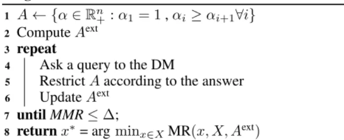
Algorithm. The idea of our algorithm is to interleave prefer-ence queries with MMR computations until the MMR value drops to zero (see Algorithm 1). Note that with the initial definition of A given in line 1 the set Aextcontains only n elements (all vectors whose i first components are equal to 1, the others being equal to zero). The answer to the preference query generated in line 4 allows a reduction of the MMR
Algorithm 1:
1 A ← {α ∈ Rn+: α1= 1 , αi≥ αi+1∀i} 2 Compute Aext
3 repeat
4 Ask a query to the DM
5 Restrict A according to the answer 6 Update Aext
7 until MMR ≤ ∆;
8 return x∗= arg minx∈XMR(x, X, Aext)
value, and this can be iterated until MMR ≤ ∆, where ∆ is a positive acceptance threshold. If ∆ = 0 then the algorithm yields an optimal solution, otherwise we only obtain a near-optimal solution. We propose below two different strategies for generating preference queries:
Strategy S1: The first strategy is focused on the fast reduc-tion of MMR values. It uses the CSS strategy recalled at the end of Section 4. It makes it possible to determine a neces-sary winner or almost necesneces-sary winner while parameter α remains largely imprecise, thus saving a lot of queries. This strategy is illustrated below on Example 1.
Example 2 (continued). If we apply Algorithm 1 to Ex-ample 2 with strategy S1, the initial uncertainty set A is pictured on Figure 1.a. To simulate the DM’s an-swers we use the weighting vector (1, 2/3, 1/3) (the dark point in the figures). The MMR value is computed a first time and we obtain MMR = 3 > 0. So, the DM is asked to compare x∗ = arg minx∈XMR(x, A, X) = (71, 50, 45) obtained from z1 = (1, 1, 1, 1, 1, 0, 0) and y∗ =arg maxy∈Xmaxα∈Afα(y) − fα(x∗) = (55, 49, 48) ob-tained fromz2= (1, 0, 1, 1, 1, 0, 1). Assume the DM prefers x∗, then we add fα(x∗) ≥ fα(y∗) to the definition of A, leading to a smaller uncertainty set pictured in Figure 1.b. The MMR value is computed again and we find MMR = 2 > 0, the DM compare x∗ = (71, 50, 45) and y∗ = (70, 61, 37) obtained from z1 and z3 = (0, 1, 1, 1, 1, 0, 1) respectively. Assume the DM still prefersx∗, then the con-straintfα(x∗) ≥ fα(y∗) is added to the definition of A. The final set A is pictured in Figure 1.c. The MMR is updated and we find MMR= 0 so the algorithm stops. By construc-tion, solutionx∗remainsfα-optimal whateverα ∈ A.
α2 α3 a. 1 1 α2 α3 b. 1 1 α2 α3 c. 1 1
Figure 1: Evolution of the uncertainty set A
Strategy S2: This strategy is focused on a methodic division of the uncertainty set, which indirectly entails a reduction of MMR values. Every component αi, i ∈J1, nK is bounded by an interval Ii = [li, ui] of possible values (initially [0, 1]). At
every step, we select the largest interval Iiand we generate a preference query enabling to remove the half of the interval. More precisely, we ask the DM to compare the two utility vectors x and y defined as follows:
x =(0, λc 1 + λ, ..., λc 1 + λ | {z } ×(i−2) , c, ..., c | {z } ×(n−i+1) ), y =( λc 1 + λ, ..., λc 1 + λ | {z } ×i , c, ..., c | {z } ×(n−i) )
and λ = (li + ui)/2 is the middle of Ii and c ∈ (0, M ]. Suppose that x is preferred to y, we deduce fα(x) ≥ fα(y) and then: λc 1+λ( i−1 P j=2 αj) + c n P j=i αj≥ 1+λλc ( i P j=1 αj) + c n P j=i+1 αj ⇒ αi≥ λ 1+λα1+ λ
1+λαi ⇒ (1 + λ)αi≥ λα1+ λαi ⇒ αi≥ λα1
Under the non-restrictive assumption that α1= 1 we obtain αi ≥ λ = (li+ ui)/2. On the other hand, whenever y is preferred to x, a similar reasoning leads to αi≤ (li+ ui)/2. In both cases we can update one of the bounds of Ii. Example 2 (continued). Let us now apply Algorithm 1 with strategy S2, the weighting vector used to simulate the DM’s answers being still(1, 2/3, 1/3). The initial uncertainty set A is the same as in Figure 1.a. and the first MMR value is 3 > 0. We have initially I2 = I3 = [0, 1], we first chose to reduceI2(arbitrarily). For this, we construct two vectors x and y as explained above (with i = 2) to generate the first preference query. The DM’s answer allows to add the constraint w2 ≥ 0.5 as pictured in Figure 2.a. The MMR value is recomputed and we still find MMR = 3 > 0 so we ask a second question to the DM aiming to reduceI3 since it is now bigger thanI2. The answer leads to the con-straintw3≤ 0.5 which is added to the definition of A (Fig-ure 2.b). The MMR is still positive. The process continue and two more questions will be necessary to obtain MMR=0 (the associated constraints are pictured in Figures 2.c and 2.d.).
α2 α3 a. 1 1 α2 α3 b. 1 1 α2 α3 c. 1 1 α2 α3 d. 1 1
Figure 2: Evolution of the uncertainty set A
This dichotomous reduction of intervals makes it possible to bound from above the number of queries necessary to ob-tain a MMR smaller than ∆. Since the utilities of the p items for the n agents belong to [0, M ], we indeed have:
Proposition 4. Algorithm 1 used with S2 and ∆ = δnpM requires at mostndlog2(1/δ)e queries for any δ ∈ (0, 1]. Proof. Let us first prove that if ui− li≤ δ for all i ∈J1, nK
then MMR ≤ ∆. Let α0be a vector arbitrary chosen in A at the current step and x0the solution maximizing fα0 over X.
For any solution y ∈ X we have:
maxα∈A{fα(y) − fα(x0)} + fα0(x0) − fα0(y)
= maxα∈A{(fα(y) − fα0(y)) − (fα(x0) − fα0(x0))}
= maxα∈A{Pni=1(αi− α0i) | {z } ≤δ y(i)− Pn i=1(αi− α 0 i) | {z } ≤δ x0(i)} ≤ δP i:αi>α0iy(i)+ δ P i:αi<α0ix 0 (i) ≤ δnpM = ∆ The term fα0(x0) − fα0(y) being positive (x0being optimal
for α0), then maxα∈A{fα(y)−fα(x0)} ≤ ∆. This reasoning being true for any solution y, then MR(x0, X, A) ≤ ∆. The MMR value being obtained by minimizing MR(x, X, A) over all x ∈ X, we obtain MMR ≤ ∆.
Moreover, note that we initially have Ii = [0, 1], for all i ∈ J1, nK due to line 1 of Algorithm 1. Hence, the itera-tive dichotomous reduction of an interval Iirequires at most dlog2(1/δ)e queries to obtain ui− li≤ δ for any i ∈J1, nK which gives ndlog2(1/δ)e overall.
Note that this bound is based on the worst case scenario. In practice it frequently happens that the MMR drops to 0 before reducing the size of all intervals to δ which saves multiple preference queries.
Example 3. If n = 10, p = 50 and M = 20 then npM = 10000 represents the range of possible fα values on subsets and therefore the range of possible MMR values. Parameter δ represents the maximal percent error allowed onfα values. If we accept a5% error (δ = 0.05) it gives ∆ = 500 and 10dlog2(1/0.05)e = 50, therefore we need at most 50 preference queries. We will see in the next section that only 17 preference queries are used on average.
7
Experimental Results
We have tested the interactive branch and bound (IBB) in-troduced in Section 5 and Algorithm 1 inin-troduced in Section 6 (used with ∆ = 0 to obtain exact solutions). To generate instances, utility and weights are generated at random us-ing an uniform density. The capacity W is randomly drawn around a reference value defined as the half of the weight of the entire set of items. This allows to favor the generation of hard knapsack instances. We generate instances of dif-ferent sizes involving up to 100 items and up to 10 agents. The DM’s answers are simulated using an hidden fα func-tion (α is randomly chosen). The linear programs formu-lated for regrets computations are solved using the Gurobi library of Python. The set Aextis computed (lines 2 and 6 of Algorithm 1) using the cdd Python’s library, which is an im-plementation of the double description method introduced in (Fukuda and Prodon 1996). The tests are performed on a Intel(R) Core(TM) i7-4790 CPU with 15 GB of RAM.
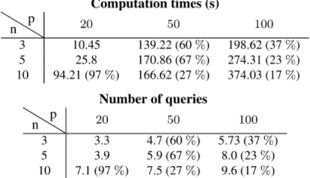
We first compare the performances of the two algorithms both in terms of computation time (in seconds) and number of preference queries (see Tables 1 and 2). The results are averaged over 30 runs with a timeout set to 20 minutes for every run. Due to the time constraint, the algorithms may be stopped before finding an optimal solution. In this case, they return the best solution found within the time window (any-time property). In particular, Algorithm 1 returns the current
Computation times (s) n p 20 50 100 3 10.45 139.22 (60%) 198.62 (37%) 5 25.8 170.86 (67%) 274.31 (23%) 10 94.21 (97%) 166.62 (27%) 374.03 (17%) Number of queries n p 20 50 100 3 3.3 4.7 (60%) 5.73 (37%) 5 3.9 5.9 (67%) 8.0 (23%) 10 7.1 (97%) 7.5 (27%) 9.6 (17%)
Table 1: Results for Interactive Branch & Bound (IBB)
Computation times (s) Number of queries n p 20 50 100 3 0.2 0.9 0.6 5 0.5 1.9 5.8 10 8.3 81.8 411.7 n p 20 50 100 3 2.7 3.9 5.3 5 2.8 6.8 11.2 10 4.7 11.2 23.1
Table 2: Results for Algorithm 1 with strategy S1
MMR solution which represents a robust choice since the gap to optimality is guaranteed to be lower than the current MMR value. In the tables below, we provide both the aver-age solution time on solved instances and the percentaver-age of solved instances within 20 minutes (when < 100%).
Tables 1 and 2 show that Algorithm 1 mostly outperforms IBB. It not only solves 100% of instances within the time constraint but runs faster on average. It also requires fewer preference queries for small or middle size instances. For big instances IBB seems to generate less preference queries but this evaluation is optimistic. The average performance only includes instances solved within the time constraint.
We next assess and compare the performances of the two elicitation strategies S1 and S2 in Algorithm 1. First S1 and S2 are compared to a random strategy S3 for the selection of preference queries. The results are given in Figure 3 that represents, for every strategy, the average MMR value (com-puted over 30 runs) as a function of the number of preference statements collected during the elicitation process.
In Figure 3 MMR values are given as a percentage of the initial MMR value computed before running the elici-tation procedure. We can see that strategies S1 and S2 are significantly more efficient that the random strategy S3, the decrease in MMR value being faster for these two strate-gies. For instance, to obtain a MMR smaller than 10% of the initial value, we need about 5 queries for S1 and ap-proximatively 17 queries for S2 while 30 preference queries would not be sufficient with S3. Wa also observed that the actual regret defined as the optimality gap achived by the current MMR solution decrease faster than the MMR val-ues. It very quickly drops to 0, which explains that we did not plot the curve on Figure 3. Moreover, we can see that S1 is significantly faster than S2 on average. This can be ex-plained as follows: Algorithm 1 implemented with S1 looks for preference queries aiming at quickly discriminating the solutions of the instance to be solved without trying to learn
Figure 3: Elicitation with S1, S2, S3 (10 agents, 50 items)
precisely vector α. Very often, a necessary winner can be identified while some components αiremain largely impre-cise. This is the key point explaining practical efficiency. Unfortunately, this approach does not provide any control on the reduction of uncertainty and prevents to derive non-trivial formal bounds on the number of queries. Algorithm 1 implemented with S2 generates queries designed to sys-tematically reduce the uncertainty attached to weights (the range of possible value is divided by two at every step), and the optimal solution is obtained as a byproduct. It allows to bound the number of queries from above but the drawback is that the generated queries may not be very efficient to de-termine the optimal choice because queries are not taylored specifically to discriminate between the solutions appearing in the particular instance to be solved. This explains why S1 empirically performs better than S2. Nevertheless, strategy S2 is also interesting because we have obtained a theoretical bound on the maximum number of queries (see Proposition 4) while keeping good empirical performances.
8
Conclusion
We proposed two active learning algorithms for the elicita-tion of weights in GSFs and the determinaelicita-tion of fα-optimal knapsacks. Algorithm 1 used with strategy S1 or S2 appears to be quite efficient, both in terms of preference queries and computation times. One research direction to further im-prove the computation of regrets concerns the control of the number of extreme points |Aext| in the uncertainty set. Al-though the exploration of Aext was easily tractable in the experiments we made, an interesting challenge would be to design new questionnaires enabling a closer control of |Aext| while keeping the informative value of our preference queries. Besides this perspective, the techniques presented here could be adapted to other fair multiagent combinato-rial optimization problems (e.g., fair assignment problems, fair multiagent scheduling problems) and more generally to elicit other decision models (linear in their parameter).
9
Acknowledgments
This work is supported by the ANR project CoCoRICo-CoDec ANR-14-CE24-0007-01.
References
Aziz, H.; Gaspers, S.; Mackenzie, S.; and Walsh, T. 2014. Fair assignment of indivisible objects under ordinal prefer-ences. In Proceedings of AAMAS-14, 1305–1312.
Benabbou, N., and Perny, P. 2015a. Combining preference elicitation and search in multiobjective state-space graphs. In Proceedings of IJCAI-15, 297–303.
Benabbou, N., and Perny, P. 2015b. Incremental weight elic-itation for multiobjective state space search. In Proceedings of AAAI-15, 1093–1099.
Benabbou, N., and Perny, P. 2016. Solving multi-agent knapsack problems using incremental approval voting. In Proceedings of ECAI-16, 1318–1326.
Benabbou, N.; Perny, P.; and Viappiani, P. 2017. In-cremental elicitation of choquet capacities for multicriteria choice, ranking and sorting problems. Artificial Intelligence 246:152–180.
Benade, G.; Nath, S.; Procaccia, A. D.; and Shah, N. 2017. Preference elicitation for participatory budgeting. In Pro-ceedings of AAAI, 376–382.
Blackorby, C., and Donalson, D. 1978. Measures of rela-tive equality and their meaning in terms of social welfare. Journal of Economic Theory2:59–80.
Bourdache, N., and Perny, P. 2017. Anytime algorithms for adaptive robust optimization with OWA and WOWA. In Proceedings of ADT-17, 93–107.
Boutilier, C.; Patrascu, R.; Poupart, P.; and Schuurmans, D. 2006. Constraint-based optimization and utility elicitation using the minimax decision criterion. Artificial Intelligence 170(8-9):686–713.
Bouveret, S., and Lang, J. 2008. Efficiency and envy-freeness in fair division of indivisible goods: Logical repre-sentation and complexity. Journal of Artificial Intelligence Research32:525–564.
Bouveret, S.; Cechl´arov´a, K.; Elkind, E.; Igarashi, A.; and Peters, D. 2017. Fair division of a graph. In Proc. of IJCAI-17, 135–141.
Braziunas, D., and Boutilier, C. 2007. Minimax regret based elicitation of generalized additive utilities. In Proc. of UAI-07, 25–32.
Brero, G.; Lubin, B.; and Seuken, S. 2018. Combinatorial auctions via machine learning-based preference elicitation. In Proceedings of IJCAI’18, 128–136.
Chajewska, U.; Koller, D.; and Parr, R. 2000. Making ratio-nal decisions using adaptive utility elicitation. In Proceed-ings of AAAI-00, 363–369.
Chevaleyre, Y.; Endriss, U.; and Maudet, N. 2017. Dis-tributed fair allocation of indivisible goods. Artificial Intel-ligence242:1–22.
Elkind, E., and Ismaili, A. 2015. Owa-based extensions of the chamberlin-courant rule. In Proc. of ADT-15, 486–502. Fluschnik, T.; Skowron, P.; Triphaus, M.; and Wilker, K. 2017. Fair knapsack. arXiv:1711.04520.
Freeman, R.; Zahedi, S. M.; and Conitzer, V. 2017. Fair and efficient social choice in dynamic settings. In Proceedings of IJCAI-17, 4580–4587.
Fukuda, K., and Prodon, A. 1996. Double description method revisited. In Comb. and Computer Science. Springer. 91–111.
Gal, Y. K.; Mash, M.; Procaccia, A. D.; and Zick, Y. 2017. Which is the fairest (rent division) of them all? J. ACM 64(6):39:1–39:22.
Galand, L., and Spanjaard, O. 2007. Owa-based search in state space graphs with multiple cost functions. In Proceed-ings of FLAIRS-07, 86–91.
Gelain, M.; Pini, M. S.; Rossi, F.; Venable, K. B.; and Walsh, T. 2010. Elicitation strategies for soft constraint problems with missing preferences: Properties, algorithms and exper-imental studies. Artificial Intelligence 174(3):270–294. Golden, B., and Perny, P. 2010. Infinite order Lorenz dom-inance for fair multiagent optimization. In Proceedings of AAMAS-10, 383–390.
Goldsmith, J.; Lang, J.; Mattei, N.; and Perny, P. 2014. Vot-ing with rank dependent scorVot-ing rules. In ProceedVot-ings of AAAI-14, 698–704.
Ha, V., and Haddawy, P. 1997. Problem-focused incremental elicitation of multi-attribute tility models. In Proceedings of UAI-97, 215–222. Morgan Kaufmann Publishers Inc. Heinen, T.; Nguyen, N. T.; and Rothe, J. 2015. Fairness and rank-weighted utilitarianism in resource allocation. In Proc. of ADT-15, 521–536.
Lesca, J., and Perny, P. 2010. LP solvable models for multia-gent fair allocation problems. In Proc. of ECAI-10, 393–398. Ogryczak, W., and ´Sliwi´nski, T. 2003. On solving linear pro-grams with the ordered weighted averaging objective. Euro-pean Journal of Operational Research148(1):80–91. Ogryczak, W. 2009. Inequality measures and equitable lo-cations. Annals of Operations Research 167(1):61–86. Skowron, P.; Faliszewski, P.; and Lang, J. 2016. Find-ing a collective set of items: From proportional multirep-resentation to group recommendation. Artificial Intelligence 241:191–216.
Wang, T., and Boutilier, C. 2003. Incremental utility elicita-tion with the minimax regret decision criterion. In Proceed-ings of IJCAI-03, 309–318.
Weng, P., and Zanuttini, B. 2013. Interactive value iteration for markov decision processes with unknown rewards. In Proceedings of IJCAI-13, 2415–2421.
Weymark, J. 1981. Generalized gini inequality indices. Math. Social Sciences1(4):409–430.
White, C. C.; Sage, A. P.; and Dozono, S. 1984. A model of multiattribute decision making and trade-off weight deter-mination under uncertainty. IEEE Transactions on Systems, Man, and Cybernetics14(2):223–229.
Yager, R. 1998. On ordered weighted averaging aggregation operators in multicriteria decision making. In IEEE Trans. Systems, Man and Cybern., volume 18, 183–190.