HAL Id: halshs-00176029
https://halshs.archives-ouvertes.fr/halshs-00176029
Submitted on 2 Oct 2007HAL is a multi-disciplinary open access archive for the deposit and dissemination of sci-entific research documents, whether they are pub-lished or not. The documents may come from teaching and research institutions in France or
L’archive ouverte pluridisciplinaire HAL, est destinée au dépôt et à la diffusion de documents scientifiques de niveau recherche, publiés ou non, émanant des établissements d’enseignement et de recherche français ou étrangers, des laboratoires
Income distribution and inequality measurement: The
problem of extreme values
Frank A. Cowell, Emmanuel Flachaire
To cite this version:
Frank A. Cowell, Emmanuel Flachaire. Income distribution and inequality measurement: The problem of extreme values. Econometrics, MDPI, 2007, 141 (2), pp.1044-1072. �10.1016/j.jeconom.2007.01.001�. �halshs-00176029�
Income Distribution and Inequality Measurement:
The Problem of Extreme Values
by
Frank A. Cowell
Sticerd, London School of Economics
and
Emmanuel Flachaire
Ces, Universit´
e Paris 1 Panth´
eon-Sorbonne
October 2006
Abstract
We examine the statistical performance of inequality indices in the presence of extreme values in the data and show that these indices are very sensitive to the properties of the income distribution. Estimation and inference can be dramatically affected, especially when the tail of the income distribution is heavy, even when stan-dard bootstrap methods are employed. However, use of appropriate semiparametric methods for modelling the upper tail can greatly improve the performance of even those inequality indices that are normally considered particularly sensitive to extreme values.
JEL classification : C1, D63
1
Introduction
There is a folk wisdom about inequality measures concerning their empirical performance. Some indices are commonly supposed to be particularly sensitive to specific types of change in the income distribution and may be rejected a priori in favour of others that are presumed to be “safer”. This folk wisdom is only partially supported by formal analysis and it is appropriate to examine the issue by considering the behaviour of inequality measures with respect to extreme values. An extreme value is a observation that is highly influential on the estimate of an inequality measure. It is clear that an extreme value is not necessarily an error or some form of contamination. It could in fact be an informative observation belonging to the true distribution – a high leverage observation. In this paper, we study sensitivity of different inequality measures to extreme values, in both cases of contamination and of high leverage observations.
What is a “sensitive” inequality measure? This issue has been addressed in ad hoc discus-sion of individual measures in terms of their empirical performance on actual data (Braulke 1983). Some of the welfare-theoretical literature focuses on transfer sensitivity (Shorrocks and Foster 1987) and related concepts. But it is clear that informal discussion is not a sat-isfactory approach for characterising alternative indices; furthermore the welfare properties of inequality measures in terms of the relative impact of transfers at different income levels will not provide a reliable guide to the way in which the measures may respond to extreme values. We need a general and empirically applicable tool.
Specifically we need to address four key issues that are relevant to assessing the sensitivity of inequality measures: 1) influence functions and their performance in presence of con-tamination; 2) sensitivity to high leverage observations; 3) error in probability of rejection in tests with finite samples; 4) sensitivity under different underlying distributions/shapes of tails. The paper will provide general results and simulation studies for each of these four topics using a variety of common inequality indices, in order to yield methods that are implementable in practice.
In section 2, we examine the sensitivity of inequality measures to contamination in the data, both in high and low incomes. In section 3, we study the sensitivity of inequality measures to “high-leverage” observations. We investigate Monte Carlo simulations to study the error in the rejection probability of a test in finite samples. Section 4 examines the relationship between the apparent sensitivity of the inequality index and the shape of the income distribution. Section 5 proposes a method for detecting extreme values in practice and section 6 concludes.
2
Data contamination
The principal tool that we use for evaluating the influence of data contamination on es-timates is the influence function (IF ), taken from the theory of robust estimation. If the
may be catastrophically affected by data contamination at z or a value close to z. Cowell and Victoria-Feser (1996) have shown that “if the mean has to be estimated from the sam-ple then all scale independent or translation independent and decomposable measures have an unbounded IF ” and that inequality measures are typically not robust to data contam-ination.1 In this section, we re-examine this negative conclusion by using a more detailed comparison of the sensitivity of inequality measures. First we demonstrate how sensitive various inequality measures are to contamination in high and small incomes (section 2.1). Then, we propose a semiparametric method of obtaining inequality measures that are much less sensitive to data contamination (section 2.2).
2.1
Sensitivity of inequality measures
The relative performance of inequality measures can be established by examining the be-haviour of the IF for each measure. We need to know the rate at which the measure approaches infinity in the region where the IF is unbounded. Fortunately, in the case of inequality measures this requires that we concentrate only on the extremes of the support of the income distribution: where data contamination occurs at a point z that is at, or close to, zero and where the contamination point z approaches infinity.
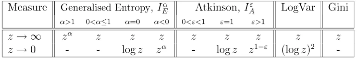
The rate of increase to infinity of the influence function for various types of inequality measures is summarised in Table 1 – for details of derivations see the Appendix. First of all, we can see that all the inequality measures discussed here have an influence function that is unbounded when z tends to infinity:2 the measures are not robust to data contamination in high incomes (Cowell and Victoria-Feser 1996). However, we can say more: the rate of increase of IF to infinity, when z tends to infinity, is faster for the Generalised Entropy (GE) measures with α > 1. In other words:
Result 1: Generalised Entropy measures with α > 1 are very sensitive to high incomes
in the data.
Furthermore, we can see that, for some measures, the IF also tends to infinity when z tends to zero: the rate of increase is faster for the GE measures with α < 0 and for the Atkinson measures with ε > 1. This result suggests that,
Result 2: Generalised Entropy measures with α < 0, and Atkinson measures with ε > 1 are very sensitive to small incomes in the data.
Using just the information in Table 1 we cannot compare the rate of increase of the IF for different values of 0 < α < 1 and 0 < ε < 1. If we do not know the income distribution,
1
The issue of data contamination is complementary to, but distinct from, the issue of measurement error that has been addressed by Chesher and Schluter (2002). These two issues typically require different estimation techniques.
2
we cannot compare the influence functions of different classes of measures, because the
IF s are functions of the moments of the distribution. However, we can choose an income
distribution and then plot and compare their influence functions for a special case. The distribution proposed by Singh and Maddala (1976), which is a member of the Burr family (type 12), is particularly useful in that it can successfully mimic observed income distri-butions in various countries (Brachman et al. 1996). The cumulative distribution function (CDF) of the Singh-Maddala distribution is
F (y) = 1 − 1
(1 + ayb)c. (1) We use the parameter values a = 100, b = 2.8, c = 1.7, which closely mirrors the net income distribution of German households, up to a scale factor. It can be shown that the moments of the distribution with CDF (1) are
E(yα) = Z ∞ 0 yαdF (y) = a−α/bΓ(1 + αb −1) Γ(c − αb−1) Γ(c) , (2)
where Γ(·) is the gamma function (see e.g. McDonald 1984). Using (2) in the definition (38) in the Appendix gives us the true values of GE measures for the Singh-Maddala distribution, from which we can derive true values of Theil and Mean Logarithmic Deviation (MLD) measures by l’Hopital’s rule,3 we obtain
E(ylog y) = µFb−1[γ(b−1+ 1) − γ(c − b−1) − log a], E(log y) = b−1[γ(1) − γ(c) − log a],
where
γ(z) := 1 Γ(z)
dΓ(z) dz .
With these moments, we can compute true values of Generalised Entropy measures. For our choice of parameter values, we have I2
E = 0.162037, IE1 = 0.140115, IE0.5 = 0.139728, I0
E = 0.146011, IE−1 = 0.189812, I −2
E = 0.386647. In addition, we approximate true values of Logarithmic Variance and Gini measures from a sample of 10 million observations drawn from the Singh-Maddala distribution: ILV = 0.332128 and IGini = 0.288714 – for formal definitions of the inequality indices see the Appendix, page 20.
In order to compare different IF s we need to normalize them. Dividing the influence function by its index we obtain the relative influence function:
RIF (I) = IF [I( ˆF )]
I( ˆF ) . (3)
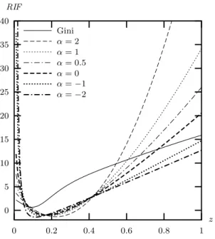
Figure 1 plots the relative influence functions for different GE measures, with α = 2, 1, 0.5, 0, −1 and for the Gini index, as functions of the contaminated value z on the x-axis. For the GE measures we can see that, when z increases, the IF increases faster
3
with high values of α ; when z tends to 0, the IF increases faster with small values of α. The IF of the Gini index increases more slowly than others but is larger for moderate values of z. In Figure 2, we plot relative influence functions for the Atkinson measures with ε = 2, 1, 0.5, 0.05, for the Logarithmic Variance and for the Gini index. For the Atkinson measures we can see the opposite relation: when z increases, the IF increases as rapidly if ε is positive and small, but when z tends to 0 the IF increases as rapidly if ε is large. The IF of the Logarithmic Variance increases slowly as z tends to infinity, but rapidly as z tends to zero. Once again, the IF of Gini index increases more slowly and is larger for moderate values of z.
A comparison of the Gini index with the Logarithmic Variance, GE or Atkinson influence functions does not lead to clear-cut conclusions a priori. In order to get a handle on the likely magnitudes involved we used a simulation study to evaluate the impact of a contam-ination in large and small observations for different measures of inequality. We simulated N = 100 samples of n = 200 observations from the Singh-Maddala distribution. We then contaminated the largest observation by multiplying it by 10 in the case of contamination in high values and by dividing the smallest observation by 10 in the case of contamination in small values. Let Yi, i = 1, . . . , n, be an IID sample from the distribution F ; ˆF is the empirical distribution function of this sample and ˆF⋆ the empirical distribution function of the contaminated sample. For each sample we compute the quantity
RC(I) = I( ˆF ) − I( ˆF ⋆)
I( ˆF ) , (4)
which evaluates the relative impact of a contamination on the index I( ˆF ). We can then plot and compare realizations of RC(I) for different measures. In order to have a plot that is easy to interpret, we sorted the samples such that realizations of RC(I) for one specific measure are increasing.
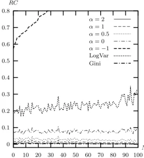
Figure 3 plots realizations of RC(I) for the Gini index, the Logarithmic Variance index and the GE measures with α = 2, 1, 0.5, 0, −1, 2, when contamination is in high values. The y-axis is RC(I) and the x-axis is the 100 different samples, sorted such that Gini realizations are increasing. Figure 4 plots realizations of RC(I) for the same measures when contamination is in small values. We can see from Figures 3 and 4 that the Gini index is less affected by contamination than the GE measures. However, the impact of the contamination on the Logarithmic Variance and GE measures with 0 ≤ α ≤ 1 is relatively small compared to measures with α < 0 or α > 1. In addition, the GE measures with 0 ≤ α ≤ 1 are less sensitive to contamination in high values if α is small. Finally, the Logarithmic Variance index is slightly less sensitive to high incomes than the Gini, but very sensitive to small incomes. To summarise:
Result 3: (a) The Gini index is less sensitive to contamination in high incomes than
the Generalised Entropy class of measures. (b) Measures in the Generalised Entropy class are less sensitive as α is small.
Corresponding results are available for the Atkinson class of measures, but with the opposite relation for its parameter (ε = 1 − α).
2.2
Semiparametric inequality measures
We have seen that inequality measures can be very sensitive to the presence of data con-tamination in high or low incomes. The standard way to compute inequality measures is to consider the empirical distribution function (EDF) as an approximation of the income distribution. In the presence of data contamination in high incomes, we suggest comput-ing inequality measures based on a semiparametric estimation of the income distribution: using the EDF for all but the right-hand tail and a parametric estimation for the upper tail. Many parametric income distributions are heavy-tailed: this is so for the Pareto, Singh-Maddala, Dagum and Generalised Beta distributions, see Schluter and Trede (2002). This means that the upper tail decays as a power function:
Pr(Y > y) ∼ βy−θ as y → ∞. (5) The index of stability θ determines which moments are finite: the mean is finite if θ > 1 and the variance is finite if θ > 2. It is thus natural to use the Pareto distribution to fit the upper tail:
F (y) = 1 − (y/y0)−θ, y > y0. (6) For instance, Schluter and Trede (2002) show that the Singh-Maddala distribution is of Pareto type for large y, with the index of stability equals to θ = bc. In our simulations, we have bc = 4.76, see (1). Note that this idea of combining a Pareto estimate of the upper tail with a nonparametric estimate of the rest of the distribution has been suggested in inequality measurement by Cowell and Victoria-Feser (2006) to obtain robust Lorenz curves and by Davidson and Flachaire (2004) with bootstrap methods.
With this approach, we need to obtain an estimate of the index of stability θ. We follow Davidson and Flachaire (2004) and make use of an estimator proposed by Hill (1975). First rank the income data in ascending order. The unknown parameter of the Pareto distribution can be estimated on the k largest incomes, for some integer k ≤ n,
ˆθ = H−1
k,n; Hk,n = k−1 k−1 X i=0
log Y(n−i)− log Y(n−k+1), (7)
where Y(j) is the jth order income of the sample. The parametric distribution is used to fit the (100 ptail)% highest incomes, that is, fewer observations than the number of observations k used for its estimation and less and less as n increases. We can compute a semiparametric inequality measure by using the moments of the semiparametric distribution: a moment m of this distribution can be expressed as a function of the corresponding moments me from the n − k lowest incomes and mp from the Pareto estimated distribution:
m = (1 − ptail) me+ ptailmp. (8) For the generalised entropy measures (GE) where α 6= 0, 1, we have:
µ∗ = 1 n ¯ n X i=1
Y(i)+ ptail ˆθy0
ˆθ − 1 and ν ∗ α = 1 n ¯ n X i=1
Y(i)α + ptail ˆθy α 0
with ¯n = n(1 − ptail). The value of the GE index is given by Iα∗
E = [ν∗α/(µ∗)α− 1]/(α2− α). Note that this semiparametric inequality measure can be computed if and only if the two moments µ∗ and ν∗
α are finite, that is, if ˆθ ≥ α.
In the two special cases of the GE measures where α = 1 (Theil index) and α = 0 (MLD index), we have respectively
ν∗ 1 = 1 n ¯ n X i=1
Y(i)log Y(i)+ ptail ˆθy0 ˆθ − 1 · log y0+ 1 ˆθ − 1 ¸ , (10) ν∗ 0 = 1 n ¯ n X i=1
log Y(i)+ ptail · log y0+ 1 ˆθ ¸ . (11)
The value of the Theil index is obtained from I1∗
E = ν∗1/µ∗ − log µ∗ and the value of the MLD index from I0∗
E = log µ∗− ν∗0. These two measures can be computed if ˆθ ≥ 1.
Different methods have been proposed to choose k appropriately (Coles 2001, Gilleland and Katz 2005). One standard approach is to plot the estimate of the Hill estimator ˆθ for different values of k and to select the value of k for which the plot is (roughly) constant. In our experiments, we use this graphical method and set the same values as Davidson and Flachaire (2004), that is, k = n/10 and y0 is the order income of rank n(1 − ptail) where ptail = 0.04 n−1/2.
Figure 5 plots realizations of RC(I) for the semiparametric GE measures with α = 2, 1, 0.5, 0, −1, when contamination is in high values. Compared to Figure 3, a plot based on the same experiment with the EDF approximation of the income distribution, that is, a special case with ptail = 0, we can see a huge decrease of all curves, which are very close to zero for all values of α < 2. It means that in our experiment all semiparametric GE measures with α < 2 are not sensitive to the contamination in high incomes. In addition, even if the RC(I) of the semiparametric generalised entropy measure with α = 2 is still significantly different from zero, it is substantially reduced compared to the same measure computed with an EDF of the income distribution.
Result 4: Inequality measures computed with a semiparametric estimation of the
in-come distribution are much less sensitive to contamination.
We might expect that the sensitivity of the semiparametric Generalised Entropy measure with α = 2 would decrease as the sample size increases. Figure 6 plots realizations of RC(I) for the semiparametric GE measure with α = 2 as the sample size n increases, when the contamination is in high values. We can see that the sensitivity of the semiparametric index to contamination decreases rapidly as the sample size increases. In this experiment, the fraction of contamination is not constant when we increase the sample size (we multiply by 10 the largest observation). In additional experiments, we hold constant the fraction of contamination. The results show that the sensitivity decreases more slowly, but the rate of decrease depends strongly on the choice of the fraction of contamination (results are not reported). Nevertheless, even when we hold the fraction of contamination constant,
semiparametric measures appear to be much less sensitive to contamination than standard measures.
Semiparametric inequality measures can be sensitive to contamination in high incomes if the sample size is small or if the influence function is highly sensitive to contamination; in such cases, we could use a robust estimate of the Pareto coefficient, as proposed by Cowell and Victoria-Feser (1996, 2006). However, our experiments suggest the remarkable conclusion that even simple non-robust methods of estimating the Pareto distribution will substantially reduce the impact of data contamination on inequality measures.
Clearly it is possible to apply the same methods of analysis to the case where there is contamination in the lower tail in order to deal with cases such as the logarithmic variance or the bottom-sensitive sub-class of the GE class of indices. However this is likely to provide only a partial story. There are two points to consider here.
First, unlike the upper-tail problem where the support of distribution is typically un-bounded above, in most cases the natural assumption is that the support of the distribution is bounded below at zero. Clearly whether this “natural” assumption is a good one or not will depend on the precise definition of income or wealth in the problem at hand.
Second, consider the way in which the data are likely to be generated and reported. In the lower tail the appropriate model for observed data may be one of the form:
y = ½
x with probability p 0 with probability 1 − p,
where x is true income that is drawn from some continuous distribution. This model clearly will generate a point mass at zero that will require treatment that is qualitatively different from that suggested above. One obvious motivation for this type of model is to be found in the income-reporting process: some individuals may (fraudulently) not report all, or may falsely claim to have no income components that fall within the definition of income. However, these false zeros are not generated exclusively by misinformation on the part of income receivers, but also by practices in the way data are recorded. Some individuals may be treated as having effectively a zero income by the procedures of the tax authority or other agency that is collecting the information because, in some sense, the income is “too small to matter.”4 Clearly this “(0, x) issue” requires a separate treatment that takes us beyond the scope of the present paper.
3
High leverage observations
An extreme value is not necessarily an error or some sort of contamination: it could be an observation belonging to the true distribution and conveying important information.
4
A variant on this data-recording problem is where the data-collection agency, recognising that there is a very small income, is unwilling to record a zero but instead assigns the income value some small positive value – one dollar, for example.
A genuine observation can be considered “extreme” in the sense that its influence on the estimate of the inequality measure is very important. Such observations can have seri-ous consequences for the statistical performance of the inequality measure and may make conventional hypothesis testing inappropriate.
We can illustrate this by reference to an index that is normally considered to be relatively “well-behaved” . Recently Davidson and Flachaire (2004) have shown that statistical tests based on the Theil index are unreliable in certain situations. In this case the cause of the unreliability appears to lie in the exact nature of the tails of the underlying distribution, in other words precisely where one expects to find high-leverage observations. Furthermore the problems persist even in large samples.
Here we want to build on the Davidson and Flachaire (2004) insight by examining the influence of high-leverage observations on a range of inequality measures. To do this we examine the statistical performance of a range of inequality measures – with Theil as a special case – using Monte Carlo simulation methods. We consider first the standard inference tools, the asymptotic and bootstrap tests for inequality (section 3.1). Then, we will look at some ways of getting round the problems that high-leverage observations cause for the standard methods (sections 3.2 and 3.3).
3.1
Asymptotic and bootstrap tests
If Yi, i = 1, . . . , n, is an IID sample from the distribution F , then the empirical distribution function of this sample is
ˆ F (y) = 1 N N X i=1 ι(Yi ≤ y). (12)
A decomposable inequality measure can be estimated by using the sample moments
µFˆ = 1 N N X i=1 Yi and νFˆ = 1 N N X i=1 φ(Yi), (13)
which are consistent and asymptotically normal, and the definition of I in terms of the moments (see the Appendix):
I( ˆF ) := ψ ( νFˆ; µFˆ). (14) This estimate is also consistent and asymptotically normal, with asymptotic variance that can be calculated by the delta method. Specifically, if ˆΣ is the estimate of the covariance matrix of νFˆ and µFˆ5, the variance estimate for I( ˆF ) is
ˆ V¡I( ˆF )¢ = £∂ψ/∂νFˆ; ∂ψ/∂µFˆ¤ Σˆ " ∂ψ/∂νFˆ ∂ψ/∂µFˆ # . (15) 5
Then, ˆΣ is a symmetric 4 × 4 matrix with arguments calculated as: ˆΣ11 = N−1P N i=1(φ(Yi) − νFˆ)2, ˆ Σ22= N− 1PN i=1(Yi− µFˆ) 2 and ˆΣ12= ˆΣ21= N− 1PN i=1(Yi− µFˆ)(φ(Yi) − νFˆ).
Using the inequality estimate (14) and the estimate (15) of its variance, it is possible to test hypotheses about I(F ) and to construct confidence intervals for it. The obvious way to proceed is to base inference on asymptotic t statistics computed using (14) and (15). Consider a test of the hypothesis that I(F ) = I0, for some given value I0. The asymptotic t statistic for this hypothesis, based on ˆI := I( ˆF ), is
W = ( ˆI − I0)/( ˆV ( ˆI))1/2, (16) where ˆV ( ˆI) denotes the variance estimate (15). We compute an asymptotic P value based on the standard normal distribution or on the Student distribution with n degrees of free-dom. For the particular case of the Gini index, its estimate is computed by
ˆ IGini = 1 µFˆ N X i=1 N X j=1 |Yi− Yj| (17)
and its standard deviation is computed as defined by Cowell (1989). An asymptotic P value is calculated from (16).
In order to construct a bootstrap test we resample from the original data. Since the test statistic we have considered so far is asymptotically pivotal, bootstrap inference should be superior to asymptotic inference.6 After computing W from the observed sample one draws B bootstrap samples, each of the same size n as the observed sample, by making n draws with replacement from the n observed incomes Yi, i = 1, . . . , n, where each Yi has probability 1/n of being selected on each draw. Then, for bootstrap sample j, j = 1, . . . , B, a bootstrap statistic W⋆
j is computed in exactly the same way as W from the original data, except that I0 in the numerator (16) is replaced by the index ˆI estimated from the original data. This replacement is necessary in order that the hypothesis that is tested by the bootstrap statistics should actually be true for the population from which the bootstrap samples are drawn, that is, the original sample (Hall 1992). This method is known as the percentile-t or bootstrap-t method. The bootstrap P value is just the proportion of the bootstrap samples for which the bootstrap statistic is more extreme than the statistic computed from the original data. Thus, for the usual two-tailed test, the bootstrap P value, P⋆, is P⋆ = 1 B B X j=1 ι(|Wj⋆| > |W |), (18)
where ι(.) is the indicator function. For the investigation carried out here, it is more revealing to consider one-tailed tests, for which rejection occurs when the statistic is too negative.
Again we simulate the data from the same Singh-Maddala distribution that was used in section 2 – see equation (1). Figure 7 shows Error in the Rejection Probability (ERP) of
6
Beran (1988) showed that bootstrap inference is refined when the quantity bootstrapped is asymptot-ically pivotal. A statistic is aymptotasymptot-ically pivotal if its asymptotic distribution is independent of the data generating process which generates the data from which the quantity is calculated. The test statistic W is aymptotically distributed as the standard normal distribution N (0, 1) and so, is asymptotically pivotal.
asymptotic tests at the nominal level 0.05, that is, the difference between the actual and nominal probabilities of rejection, for different GE measures, for the Logarithmic Variance index and for the Gini index, when the sample size increases.7 The plot for a statistic that yields tests with no size distortion coincides with the horizontal axis. Let us take an example from Figure 7: for n = 2,000 observations, the ERP of the GE measure with α = 2 is approximately equal to 0.11: it means that asymptotic test over-rejects the null hypothesis and that the actual level is 16%, when the nominal level is 5%. In our simulations, the number of replications is 10,000. From Figure 7, it is clear that the ERP of asymptotic tests is very large in moderate samples and decreases very slowly as the sample size increases; the distortion is still significant in very large samples. We can see that the Gini index, the Logarithmic Variance and the GE measure with α = 0 perform similarly. Because of the high ERP for some of the GE indices we carried out some additional experiments with two extremely large samples, 50,000 and 100,000 observations. The results are shown in Table 2 from which we can see that the actual level is still nearly twice the nominal level for GE measures with α = 2. The distortion is very small in this case only for α = 0 and 0.5. Figure 8 shows the ERPs of bootstrap tests. Firstly, we can see that distortions are reduced for all measures when we use the bootstrap. However, the ERP of the GE measure with α = 2 is still very large even in large samples, the ERPs of GE measure with α = 1, 0.5, −1 are small only for large samples. The GE measure with α = 0 (the MLD) performs better than others and its ERP is quite small for 500 or more observations. These results suggest that,
Result 5: The rate of convergence to zero of the error in the rejection probability
of asymptotic and bootstrap tests is very slow. Tests based on Generalised Entropy measures can be unreliable even in large samples.
Computations for the Gini index are very time-intensive and we computed ERPs of this index only for n = 100; 500; 1,000 observations: we found ERPs similar to those of the GE index with α = 0. Experiments on the Logarithmic Variance index show that it performs similarly to the Gini index and the GE measure with α = 0. For the Atkinson class of measures, we again find results similar to those for the GE with ε = 1 − α. These results lead us to conclude that,
Result 6: The Generalised Entropy with α = 0, Atkinson with ε = 1, Logarithmic
Variance and Gini indexes perform similarly in finite samples.
3.2
Non-standard bootstraps
As we noted earlier, the major cause of the poor performance of the standard bootstrap method in the case of the Theil index is its sensitivity to the nature of the upper tail of the distribution: income distributions are often heavy-tailed distributions. Davidson and
7
Flachaire (2004) suggested two non-standard methods of bootstrapping a heavy-tailed dis-tribution: the m out of n bootstrap – known as the moon bootstrap – and a semiparametric bootstrap. Their simulation results suggest that the semiparametric bootstrap gives ac-curate inference in moderately large samples and it leads us to study these two methods using a broader class of inequality measures.
The m out of n bootstrap is a technique based on drawing subsamples of size m < n. However, the choice of the size of the bootstrap samples m can be a problem, particularly for skewed distributions (Hall and Yao 2003). Income distributions are generally highly skewed and Davidson and Flachaire (2004) have shown that the ERP is very sensitive to the choice of m. In the light of this they propose the computation of the P -value bootstrap as follows:
Pmoon = Φ(w) + ˆan−1/2, (19) where w is a realisation of the statistic W and ˆa is given by
ˆ
a = p(m, n) − p(n, n)
m−1/2− n−1/2 (20) when p(m, n) and p(n, n) are the P -values given respectively by the moon and standard bootstraps. Unlike the moon bootstrap P -value, Davidson and Flachaire’s Pmoon is not very sensitive to the choice of m: they use m = n1/2 in their experiments. Figure 9 shows ERP of moon bootstrap tests as defined in (19) and (20), with m = n1/2. Compared to the ERP of standard bootstrap tests in Figure 8, we can see that distortions are reduced for all measures in small samples. However, the ERPs are quite similar in the two figures, for samples with n = 2000 or more observations.
Result 7: The moon bootstrap performs better than the standard bootstrap in small
samples. However, these two bootstrap methods perform similarly in moderate and large samples.
The semiparametric bootstrap is similar to the standard bootstrap for all but the right-hand tail where a Pareto distribution is used to represent the distribution. With probability 1 − ptail, an element of a bootstrap sample is drawn with replacement from the n − k lowest incomes, for some integer k ≤ n. With probability ptail, an element of a bootstrap sample is drawn from the Pareto distribution, defined in (6), where the unknown parameter θ is estimated as proposed by Hill (1975), defined in (7). In our simulations, we set k = n/10 and ptail = 0.04 n−1/2. Figure 10 shows ERP of semiparametric bootstrap tests. Compared to the ERP of the standard and of the moon bootstrap tests in Figures 8 and 9, we can see that distortions are largely reduced for all generalised entropy measures with α > 0, that is, for all measures insensitive to small incomes (see Table 1). Results for the MLD index (the case α = 0) are not as clear, but we will see in the next section that this result can be clearly drawn for this index too, when we consider different choice of the shape of the income distribution.
Result 8: The semiparametric bootstrap outperforms the standard and the moon
3.3
Semiparametric inequality measures
We considered earlier inequality measures computed with the EDF of the income distri-bution (nonparametric measures). In this subsection, we examine inequality measures computed with a semiparametric estimation of the income distribution (semiparametric measures), as suggested in section 2.2.
Let us consider the semiparametric Generalised Entropy measures, as defined in (9), (10) and (11). To make inference, we need to derive the standard errors of these measures. The variance can be obtained from (15) where we replace ˆΣ by ˆΣ∗
α, the estimate of the covariance matrix of µ∗ and ν∗
α. If we consider α 6= 0, 1, we have ˆ Σ∗ α = " ν∗ 2 − (µ∗)2 ; ν∗α+1 − µ∗ν∗α ν∗ α+1 − µ∗ν∗α ; ν∗2α− (ν∗α)2 # . (21)
For the case of α = 0 (MLD index) and α = 1 (Theil index), we have
ˆ Σ∗ 0 = " ν∗ 2− (µ∗)2 ; ν∗1− µ∗ν∗0 ν∗ 1 − µ∗ν∗0 ; ν∗a− (ν∗0)2 # and Σˆ∗ 1 = " ν∗ 2− (µ∗)2 ; ν∗c − µ∗ν∗1 ν∗ c − µ∗ν∗1 ; ν∗b − (ν∗1)2 # . (22)
Deriving the corresponding moments from the Pareto distribution and using (8), we obtain
ν∗ a= 1 n ¯ n X i=1
[log Y(i)]2+ ptail · (log y0)2+2 ˆθ µ log y0+ 1 ˆθ ¶¸ , (23) ν∗ b = 1 n ¯ n X i=1
[Y(i)log Y(i)]2+ ptail " ˆθ(y0log y0)2 ˆθ − 2 + 2ˆθy2 0 (ˆθ − 2)2 µ log y0+ 1 ˆθ − 2 ¶# , (24) ν∗ c = 1 n ¯ n X i=1
Y(i)2 log Y(i)+ ptail " ˆθy2 0 ˆθ − 2 µ log y0+ 1 ˆθ − 2 ¶# . (25)
The standard error can be computed if and only if all the relevant moments are finite. This requires that, for given α:
ˆθ ≥ max{2, 2α}. (26) This condition highlights a major issue in the use of such semiparametric measures: they cannot be used in practice if ˆθ is too small or α is too large. The value of ˆθ is an estimate of the index of stability: this index is small if the distribution is strongly heavy-tailed. It is clear from condition (26) that the term “strongly heavy-tailed” subsumes two points. First, if the estimate ˆθ < 2, then nothing can be done with the semi-parametric method, Second, if ˆθ ≥ 2 but is less than 2α, then one is violating a self-imposed constraint con-tingent on the choice of α: if one wants to use the semi-parametric method then it is necessary to choose an inequality measure with a lower value of α. This second part of the restriction makes sense intuitively: in trying to use a high value of α one is trying to make the inequality index particularly sensitive to the information in the upper tail.
Furthermore the semi-parametric approach may raise problems in applying the bootstrap method, because for each bootstrap sample we need to estimate a new value ˆθ: even if con-dition (26) is satisfied in the original sample, it can be violated many times in bootstrap samples. For this reason we will consider asymptotic tests, that is, a test statistic com-puted with the semiparametric inequality measures as defined above with the asymptotic distribution as the nominal distribution.
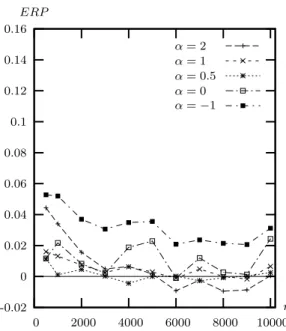
Figure 11 shows ERP of asymptotic tests based on semiparametric inequality measures. Compared to the ERP of asymptotic tests based on nonparametric inequality measures (Figure 7), we can see that distortions are largely reduced for all generalised entropy mea-sures with α ≥ 0. Compared to the ERP of semiparametric bootstrap tests based on nonparametric inequality measures (Figure 10), we can see that distortions are very similar for 0 ≤ α < 2 and significantly reduced for the case α = 2.
Condition (26) holds for GE measures with α ≤ 1 if and only if ˆθ ≥ 2 and for the case α = 2 if and only if ˆθ ≥ 4. In all our experiments, we can calculate semiparametric GE measures with α ≤ 1. However, this is not true for the case α = 2 and, depending on the sample size, the attempt at computing the semiparametric index may fail. The relationship between n, the sample size, and δ the percentage of cases where a semiparametric index cannot be computed in the Monte-Carlo experiments, is presented in Table 3. In our simulations, we do not compute the GE measure with α = 2 when condition (26) is not satisfied.
Result 9: Compared to the semiparametric bootstrap approach, asymptotic tests
com-puted with semiparametric inequality measures perform: (1) similarly for generalised entropy measures with 0 ≤ α ≤ 1, (2) better for higher values of α. However, semipara-metric measures may not be computable if α is too large or if the income distribution is too heavy-tailed.
The question remains as to whether our reliance on simulation means that the results established in this section are particular to a special case of a special family of income distributions. The next section addresses this question.
4
The shape of the income distribution
Some of the results on contamination and high-leverage observations are based on a specific choice of the income distribution: the Singh-Maddala distribution with a special choice of parameters. In this section, we examine the robustness of our conclusions by extending some of the key results to cases with other choices of parameters and of distributions. In addition to the Singh-Maddala, we use the Pareto and the Lognormal functional forms, both of which have wide application in the modelling of income distributions.
The CDF of the Singh-Maddala distribution is defined in (1). In our simulation, we use a = 100, b = 2.8 and c = 0.7, 1.2, 1.7. The upper tail is thicker as c decreases.
The CDF of the Pareto distribution (type I) is defined by
Π(y ; yl, θ) = 1 −³yl y
´θ
, (27)
where yl > 0 is a scale parameter and θ > 0 is the Pareto coefficient. The formulas for the Theil and MLD measures, given that the underlying distribution is Pareto, are respectively
IE1(Π) = 1 θ − 1 + log θ − 1 θ and I 0 E(Π) = − 1 θ − log θ − 1 θ (28) (Cowell 1995). In our simulation, we use yl = 0.1 and θ = 1.5, 2, 2.5. The upper tail is thicker as θ decreases.
The CDF of the Lognormal distribution is defined by
Λ(y ; µ, σ2) = Z y 0 1 √ 2πσxexp ³ − 1 2σ2[log x − µ] 2´dx. (29)
The formulas for Theil and Mean Logarithmic Deviation (MLD) measures, given that the underlying distribution is Lognormal, are both equal to
IE1(Λ) = IE0(Λ) = σ2/2, (30) see Cowell (1995). In our simulation, we use µ = −2 and σ = 1, 0.7, 0.5. The upper tail is thicker as σ increases.
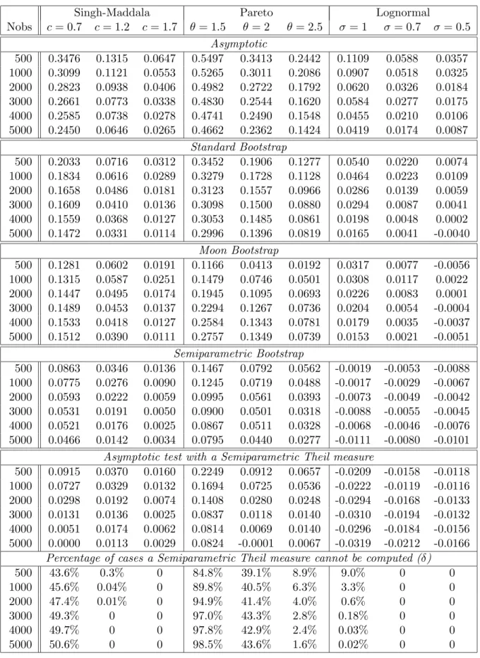
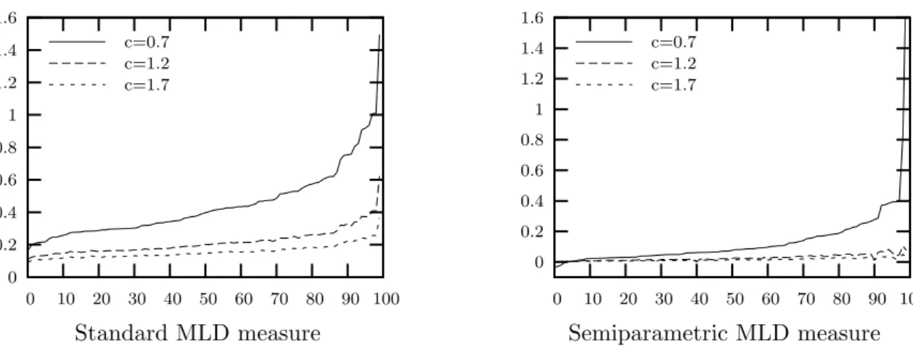
As described in section 2 at Figure 3, we use a similar simulation study to evaluate the impact of a contamination in large observations for the MLD index and for the different underlying distributions described above. Figures 13, 14 and 15 respectively plot the dif-ference I( ˆF ) −I( ˆF⋆) of our three different choices of parameters for Singh-Maddala, Pareto and Lognormal distributions. We consider standard measures - computed with the EDF of the income distribution - and semiparametric measures (see section 2.2). In all cases, we can see that the MLD index is more sensitive to contamination when the upper tail is heavy, that is to say thick (c = 0.7, θ = 1.5, σ = 1), and less sensitive when the upper tail is thin (c = 1.7, θ = 2.5, σ = 0.5). It is also clear that semiparametric measures are much less sensitive to contamination.
Result 10: The Mean Logarithmic Deviation index is more sensitive to contamination
in high incomes when the underlying distribution upper tail is heavy. Semiparametric MLD measures are much less sensitive.
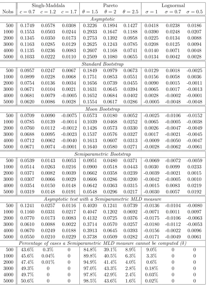
As described in section 3, we study statistical performance of Theil and MLD measures for the different underlying distributions described above. Tables 4 and 5 gives result of ERPs of asymptotic and bootstrap tests for the Theil and MLD inequality measures. Column 4, Singh-Maddala with c = 1.7 is similar to the curve labelled α = 0 in Figure 7. From these tables, we can draw the following conclusions:
1. ERP is quite large and decreases slowly as the number of observations increases 2. ERP is more significant with heavy upper tails (c = 0.7, θ = 1.5, σ = 1) than with
thin upper tails (c = 1.7, θ = 2.5, σ = 0.5)
3. ERP is smaller with the Lognormal than with Singh-Maddala distributions; in turn the ERP is smaller with Singh-Maddala distributions than with Pareto distributions8 4. Semiparametric methods - semiparametric bootstrap tests computed with a standard measure and asymptotic tests computed with a semiparametric measure - outperform the other methods.
Note that, strictly speaking, only the moon bootstrap method is valid in the case of Pareto distribution with parameter θ = 1.5, 2 (columns 4 and 5). The reason for this is that the variance of the Pareto distribution is infinite in all cases where θ ≤ 2. In the case where θ = 1.5 it is indeed clear from column 4 that asymptotic and standard bootstrap methods give very poor results, but ERP is still largely reduced by the use of the semiparametric bootstrap. In such cases, semiparametric inequality measures can be computed in very few cases.
Result 11: The ERP of an asymptotic and bootstrap test based on the Mean
Logarith-mic Deviation or Theil index is more significant when the underlying distribution upper tail is heavy. Semiparametric methods outperforms the other methods.
5
Detection of extreme values
In our discussion so far we have referred to extreme values – whether they are contamination or genuine high-leverage observations – without being specific about how they are to be distinguished in practice from the mass of observations in the sample. Clearly this is a matter requiring quite fine judgment, but the following common-sense approach should be useful in exercising this judgment.
Consider the sensitivity of the index estimate to influential observations, in the sense that deleting them would change the estimate substantially. The effect of a single observation on ˆI can be seen by comparing ˆI with ˆI(i), the estimate of I(F ) that would be obtained if we used a sample from which the ith observation had been omitted. Let us define bIF
i as a measure of the influence of observation i, as follows:
c
IFi = ( ˆI − ˆI(i))/ ˆI. (31) Figure 12 plots the values of cIFi for different inequality measures and for the 10 highest, the 10 in the middle and the 10 smallest observations of a sorted sample of n = 5,000
8
Lognormal upper tails are known to decrease faster, as exponential functions, than Singh-Maddala and Pareto distributions, which decrease as power functions
observations drawn from the Singh-Maddala distribution, then the x-axis represents 30 ob-servations: i = 1, . . . , 10, 2495, . . . , 2505, . . . , 4990, . . . , 5000. We can see that observations in the middle of the sorted sample do not affect estimates compared to smallest or highest observations. Moreover, we can see that the highest values are more influential than the smallest values. Furthermore, we can see that the highest value is very influential for the GE measure with α = 2: its estimate should be modified by nearly 0.018 when we remove it; respectively more influential than GE with α = 1, α = 0.5, α = 0, α = −1 and the Gini index. On the other hand the GE index with α = −1 is highly influenced by the smallest observation.
Finally, this plot can be useful in practice for identifying extreme values that may sub-stantially affect inequality estimates. This can then assist in the choice of an appropriate inequality measure in the light of our previous results on sensitivity to contamination and the impact of high-leverage observations. Note that it does not tell us how one would distinguish between contamination and high leverage observations in practice. However, unless we have some specific information about the data set, it is not possible to distinguish between a leverage observation and a contamination. This problem becomes a minor issue since we can use practical methods performing well in both cases - of contamination and of leverage observation. Such practical methods are the main contribution of the paper.
6
Conclusion
Very large incomes matter both in principle and practice when it comes to inequality judgments. This is true both in cases where the extreme values are genuine observations and where they represent some form of data contamination. But practical methods that appropriately take account of the problems raised by extreme values are still relatively hard to come by.
In this paper we have demonstrated a practical way of detecting the potential problem of sensitivity to extreme values9 – see section 5. However, our analysis of the relative performance of inequality indices can be used to make four broader points that may assist in the development of empirical methods of inequality analysis.
First, semiparametric inequality measures – i.e. inequality measures based on a parametric-tailed estimation of the income distribution – are much less sensitive to contamination than those based directly on the EDF. This is true even where relatively unsophisticated methods are used for estimating the distribution that is used in the tail.
Second, bootstrap methods are often useful, but some bootstrap methods can be catas-trophically misleading. The bootstrap certainly works better than asymptotic methods but, given the typical heavy-tailed shape of the income distribution, the standard boot-strap often performs badly: indeed for some important cases the standard bootboot-strap is actually invalid.10 This negative conclusion applies to several commonly-used inequality
9
For an alternative approach see Schluter and Trede (2002).
10
measures. However, the problem can be overcome by using a non-standard bootstrap; in particular the semiparametric bootstrap outperforms the other methods and gives accurate inference in finite samples.
Third, in situations where semiparametric inequality measures can be used, they perform well in asymptotic tests and at least as well as semiparametric bootstrap methods.
Fourth, empirical researchers sometimes want to select an appropriate inequality measure on the basis of its performance with respect to extreme values: our analysis throws some light on the argument here. For example it has been suggested that the Gini coefficient is going to be less prone to the influence of outliers than some of the alternative candidate inequality indices. As might be expected the Gini coefficient is indeed less sensitive than GE indices to contamination in high incomes. However, in terms of performance in finite samples there is little to choose between the Gini coefficient and the GE index with α = 0 (or equivalently the Atkinson index with ε = 1); there is also little to choose between the Gini and the logarithmic variance. This is always true for estimation methods using the EDF; but if one uses semiparametric methods then one has an even stronger result. In such cases the apparent empirical advantage of the Gini coefficient of the alternatives virtually disappears.
References
Beran, R. (1988). “Prepivoting test statistics: a bootstrap view of asymptotic refinements”.
Journal of the American Statistical Association 83 (403), 687–697.
Brachman, K., A. Stich, and M. Trede (1996). “Evaluating parametric income distribution models”. Allgemeines Statistisches Archiv 80, 285–298.
Braulke, M. (1983). An approximation to the Gini coefficient for population based on sparse information for sub-groups. Journal of Development Economics 2 (12), 75–81.
Chesher, A. and C. Schluter (2002). “Welfare measurement and measurement error”.
Re-view of Economic Studies 69, 357–378.
Coles, S. (2001). An Introduction to Statistical Modeling of Extreme Values. London: Springer.
Cowell, F. A. (1989). “Sampling variance and decomposable inequality measures”. Journal
of Econometrics 42, 27–42.
Cowell, F. A. (1995). Measuring Inequality. 2nd edition, Harvester Wheatsheaf, Hemel Hempstead.
Cowell, F. A. and M.-P. Victoria-Feser (1996). “Robustness properties of inequality mea-sures”. Econometrica 64, 77–101.
Cowell, F. A. and M.-P. Victoria-Feser (2006). “Robust Lorenz curves: a semi-parametric approach”. Journal of Economic Inequality, forthcoming.
θ <2, a parameter range that is relevant for many practical examples of the distribution of wealth and of high incomes.
Davidson, R. and E. Flachaire (2004). “Asymptotic and bootstrap inference for inequality and poverty measures”. working paper Greqam 2004-20.
Gilleland, E. and R. W. Katz (2005). Extremes toolkit: Weather and climate applications of extreme value statistics. R software and accompanying tutorial.
Hall, P. (1992). The Bootstrap and Edgeworth Expansion. Springer Series in Statistics. New York: Springer Verlag.
Hall, P. and Q. Yao (2003). “Inference in arch and garch models with heavy-tailed errors”. Econometrica 71, 285–318.
Hampel, F. R. (1968). Contribution to the Theory of Robust Estimation. Ph. D. thesis, University of California, Berkeley.
Hampel, F. R. (1974). “The influence curve and its role in robust estimation”. Journal of
the American Statistical Association 69, 383–393.
Hampel, F. R., E. M. Ronchetti, P. J. Rousseeuw, and W. A. Stahel (1986). Robust
Statis-tics: The Approach Based on Influence Functions. New York: John Wiley.
Hill, B. M. (1975). “A simple general approach to inference about the tail of a distribution”.
Annals of Statistics 3, 1163–1174.
McDonald, J. B. (1984). “Some generalized functions for the size distribution income”.
Econometrica 52, 647–663.
Monti, A. C. (1991). “The study of the gini concentration ratio by means of the influence function”. Statistica 51, 561–577.
Schluter, C. and M. Trede (2002). “Tails of Lorenz curves”. Journal of Econometrics 109, 151–166.
Shorrocks, A. F. and J. E. Foster (1987). Transfer-sensitive inequality measures. Review of
Economic Studies 54, 485–498.
Singh, S. K. and G. S. Maddala (1976). “A function for size distribution of incomes”.
Econometrica 44, 963–970.
A
Inequality Measures and the Influence Function
Let y be a random variable – for example income – and F its probability distribution. We define the two moments
µF = Z
y dF (y) and νF = Z
φ(y) dF (y). (32)
An inequality measure fulfilling the property of decomposability can be written as
I(F ) = Z
where f is a function IR2 → IR which is monotonic increasing and concave in its first argument in order to respect the principle of transfers – see Cowell and Victoria-Feser (1996). We can also express most of the commonly-used indices as a function of the two moments µF and νF,
I(F ) = ψ ( νF; µF), (33) where φ and ψ are functions IR2 → IR and ψ is monotonic increasing in its first argument. For example this is true for the Generalised Entropy, Theil, MLD and Atkinson measures. However, the Gini index does not belong to the class of decomposable measure and cannot be reduced to the form (33): this important index will be treated separately below.
The influence function11 is defined as the effect of an infinitesimal proportion of “bad” observations on the value of the estimator. Define the mixture distribution
Gǫ = (1 − ǫ)F + ǫH, (34) where 0 < ǫ < 1 and H is some perturbation distribution; take H to be the cumulative distribution function which puts a point mass 1 at an arbitary income level z:
H(y) = ι(y ≥ z), (35) where ι(.) is a Boolean indicator – it takes the value 1 if the argument is true and 0 if it is false. The influence of an infinitesimal model deviation on the estimate is given by limǫ→0[(I(Gǫ) − I(F ))/ǫ], or ∂I(Gǫ)/∂ǫ|ǫ=0 when the derivative exists. Then, the influence function for an inequality measure defined as (33), is given by
IF (z ; I, F ) = ∂ψ ∂νGε ∂νGǫ ∂ǫ ¯ ¯ ¯ ǫ=0 + ∂ψ ∂µGε ∂µGǫ ∂ǫ ¯ ¯ ¯ ǫ=0. From (32) and (34), we have
νGǫ = (1 − ǫ)
Z
φ(y) dF (y) + ǫφ(z) and µGǫ = (1 − ǫ)
Z
y dF (y) + ǫz. (36)
Then, using (36) in (33) leads to
IF (z ; I, F ) = ∂ψ ∂νF · £ φ(z) − νF ¤ + ∂ψ ∂µF · £ z − µF¤. (37)
If the IF is unbounded for some value of z then the estimate of the index may be catastroph-ically affected by data-contamination at income values close to z. In standard asymptotic theory, the dominant power of the sample size n of an asymptotic expansion is commonly used as an indicator of the rate of convergence of an estimator. Similarly, as an indicator of the rate of increase of the IF to infinity, we can use the dominant power of z in (37).
11
The use of the IF to assess the robustness properties of any estimator originated in the work of Hampel (1968, 1974) and was further developed in Hampel et al. (1986). Cowell and Victoria-Feser (1996) used it to study robustness properties of inequality measures.
In the light of this consider the impact of an extreme value on inequality. To assess this we require the influence function for an observation at arbitrary point z and the rate of increase to infinity of IF for specific inequality measures.
• Generalised Entropy (GE) class (α 6= 0, 1)
IEα = Z 1 α(α − 1) h³ y µ ´α − 1idF (y) = 1 α(α − 1) ³ ν µα − 1 ´ , (38)
where ν =R yαdF (y). From (37) we can derive its influence function,
IF (IEα) = hzα− νi− ν (α − 1)µα+1
h
z − µi. (39)
For any given value of α the influence function is unbounded: if α > 1 then IF tends to infinity when z → ∞ at the rate of zα; if 0 < α < 1 then IF tends to infinity when z → ∞ at the rate of z; if α < 0 then IF tends to infinity when z → ∞ at the rate of z, and when z → 0 at the rate of zα.
• Theil index: this is the special case of the GE class where α = 1, IE1 = Z y µlog ³ y µ ´ dF (y) = ν µ− log µ, (40) where ν =R y log y dF (y). From (37) we can derive its influence function,
IF (IE1) = 1 µ h z log z − νi−ν + µ µ2 h z − µi. (41) This influence function tends to infinity at the rate of z when z → ∞.
• Mean Logarithmic Deviation (MLD) : this is the special case of the GE class where α = 0, IE0 = − Z log³ y µ ´ dF (y) = logµ − ν, (42) where ν =R log y dF (y). From (37) we can derive its influence function,
IF (IE0) = −hlogz − νi+ 1 µ h
z − µi. (43) This influence function tends to infinity at the IF rate of z when z → ∞ and at the rate of log z when z → 0. • Atkinson class (ε > 0) IAε = 1 −h Z ³ y µ ´1−ε dF (y)i 1 1−ε = 1 − ν 1 1 −ε µ ε 6= 1, (44) where ν =R y1−εdF (y). From (37) we can derive its influence function,
IF (IAε) = ν ε 1 −ε (ε − 1)µ h z1−ε− νi+ ν 1 1 −ε µ2 h z − µi. (45)
If 0 < ε < 1 then IF tends to infinity when z → ∞ at the rate of z. If ε > 1: IF tends to infinity when z → ∞ at the rate of z, and when z → 0 at the rate of z1−ε.12
For ε = 1, the Atkinson index is equal to
IA1 = 1 − e−IE0 = 1 − e
ν
µ, where ν = Z
log y dF (y), (46)
and its influence function is
IF (IA) = −1 e ν µ h logz − νi+ e ν µ2 h z − µi, (47)
which tends to infinity, when z → ∞ at the rate of z, and when z → 0 at the rate of log z. • Logarithmic Variance
ILV =Z hlog³ y µ
´i2
dF (y) = ν1− 2 ν2log µ + (log µ)2, (48)
where ν1 = R
(log y)2dF (y) and ν 2 =
R
log y dF (y). By extension of (37) to three parame-ters, we derive its influence function as
IF (ILV) = £ (log z)2− ν1 ¤ − 2 log µ£log z − ν2 ¤ − µ2(ν2− log µ) £ z − µ¤, (49)
which tends to infinity at the rate of z when z → ∞, and when z → 0 at the rate of (log z)2. • Gini index: there are several equivalent forms of this index, the most useful here is
IGini = 1 − 2R(F ) with R(F ) = 1 µ
Z 1
0
C(F ; q) dq (50)
where, for all 0 ≤ q ≤ 1, the Quantile function Q(F ; q) and the Cumulative income function C(F ; q) are respectively defined by
Q(F ; q) = inf©y|F (y) ≥ qª and C(F ; q) =
Z Q(F ;q) 0
y dF (y). (51)
The IF of IGini is given by (see e.g. Monti 1991)
IF (IGini) = 2 · R(F ) − C¡F ; F (z)¢+ z µ ³ R(F ) −¡1 − F (z)¢´ ¸ , (52)
which tends to infinity at the rate of z when z → ∞.
12
Note that the Atkinson index Iε
A is ordinally equivalent to the Generalised Entropy index I α E for
ε= 1 − α > 0, and is a non-linear transformation of the latter: Iε
A= 1 − [(α 2
− α)IEα+ 1]
1 α.
Measure Generalised Entropy, Iα
E Atkinson, IAε LogVar Gini α>1 0<α≤1 α=0 α<0 0<ε<1 ε=1 ε>1
z → ∞ zα z z z z z z z z
z → 0 - - log z zα - log z z1−ε (log z)2
-Table 1: Rates of increase to infinity of the influence function
n α = 2 α = 1 α = 0.5 α = 0 α = −1 50,000 0.0492 0.0096 0.0054 0.0024 0.0113 100,000 0.0415 0.0096 0.0052 0.0043 0.0125
Table 2: ERP of asymptotic tests for GE measures
n 500 1000 2000 3000 4000 5000 6000 7000 8000 9000 10000 δ (%) 27.7 22.8 17.6 14.9 12.8 10.9 10.1 9.5 7.8 7.6 6.9
Singh-Maddala Pareto Lognormal Nobs c= 0.7 c= 1.2 c= 1.7 θ= 1.5 θ= 2 θ= 2.5 σ= 1 σ = 0.7 σ= 0.5 Asymptotic 500 0.3476 0.1315 0.0647 0.5497 0.3413 0.2442 0.1109 0.0588 0.0357 1000 0.3099 0.1121 0.0553 0.5265 0.3011 0.2086 0.0907 0.0518 0.0325 2000 0.2823 0.0938 0.0406 0.4982 0.2722 0.1792 0.0620 0.0326 0.0184 3000 0.2661 0.0773 0.0338 0.4830 0.2544 0.1620 0.0584 0.0277 0.0175 4000 0.2585 0.0738 0.0278 0.4741 0.2490 0.1548 0.0455 0.0210 0.0106 5000 0.2450 0.0646 0.0265 0.4662 0.2362 0.1424 0.0419 0.0174 0.0087 Standard Bootstrap 500 0.2033 0.0716 0.0312 0.3452 0.1906 0.1277 0.0540 0.0220 0.0074 1000 0.1834 0.0616 0.0289 0.3279 0.1728 0.1128 0.0464 0.0223 0.0109 2000 0.1658 0.0486 0.0181 0.3123 0.1557 0.0966 0.0286 0.0139 0.0059 3000 0.1609 0.0410 0.0136 0.3098 0.1500 0.0880 0.0294 0.0087 0.0041 4000 0.1559 0.0368 0.0127 0.3053 0.1485 0.0861 0.0198 0.0048 0.0002 5000 0.1472 0.0331 0.0114 0.2996 0.1396 0.0819 0.0165 0.0041 -0.0040 Moon Bootstrap 500 0.1281 0.0602 0.0191 0.1166 0.0413 0.0192 0.0317 0.0077 -0.0056 1000 0.1315 0.0587 0.0251 0.1479 0.0746 0.0501 0.0308 0.0117 0.0022 2000 0.1447 0.0495 0.0174 0.1945 0.1095 0.0693 0.0226 0.0083 0.0001 3000 0.1489 0.0453 0.0137 0.2294 0.1267 0.0736 0.0204 0.0054 -0.0004 4000 0.1533 0.0418 0.0127 0.2584 0.1343 0.0781 0.0179 0.0035 -0.0037 5000 0.1512 0.0390 0.0111 0.2757 0.1349 0.0739 0.0153 0.0021 -0.0051 Semiparametric Bootstrap 500 0.0863 0.0346 0.0136 0.1467 0.0792 0.0562 -0.0019 -0.0053 -0.0088 1000 0.0775 0.0276 0.0090 0.1245 0.0719 0.0488 -0.0017 -0.0029 -0.0067 2000 0.0593 0.0222 0.0059 0.0995 0.0561 0.0393 -0.0073 -0.0049 -0.0042 3000 0.0531 0.0191 0.0050 0.0900 0.0501 0.0318 -0.0088 -0.0055 -0.0045 4000 0.0521 0.0176 0.0025 0.0867 0.0511 0.0328 -0.0068 -0.0046 -0.0076 5000 0.0466 0.0142 0.0034 0.0795 0.0440 0.0277 -0.0111 -0.0080 -0.0101
Asymptotic test with a Semiparametric Theil measure
500 0.0915 0.0370 0.0160 0.2249 0.0912 0.0657 -0.0209 -0.0158 -0.0118 1000 0.0727 0.0329 0.0132 0.1694 0.0725 0.0536 -0.0222 -0.0119 -0.0116 2000 0.0298 0.0192 0.0074 0.1408 0.0280 0.0248 -0.0294 -0.0168 -0.0133 3000 0.0131 0.0136 0.0025 0.0837 0.0118 0.0140 -0.0310 -0.0194 -0.0132 4000 0.0051 0.0174 0.0062 0.0814 0.0069 0.0140 -0.0296 -0.0184 -0.0156 5000 0.0000 0.0113 0.0029 0.0824 -0.0001 0.0067 -0.0319 -0.0212 -0.0166
Percentage of cases a Semiparametric Theil measure cannot be computed (δ)
500 43.6% 0.3% 0 84.8% 39.1% 8.9% 9.0% 0 0 1000 45.6% 0.04% 0 89.8% 40.5% 6.3% 3.3% 0 0 2000 47.4% 0.01% 0 94.9% 41.4% 4.0% 0.6% 0 0 3000 49.3% 0 0 97.0% 43.3% 2.8% 0.18% 0 0 4000 49.7% 0 0 97.8% 42.9% 2.4% 0.03% 0 0 5000 50.6% 0 0 98.5% 43.6% 1.6% 0.02% 0 0
Singh-Maddala Pareto Lognormal Nobs c= 0.7 c= 1.2 c= 1.7 θ= 1.5 θ= 2 θ= 2.5 σ= 1 σ= 0.7 σ = 0.5 Asymptotic 500 0.1749 0.0578 0.0308 0.3226 0.1894 0.1427 0.0418 0.0238 0.0186 1000 0.1553 0.0503 0.0244 0.2933 0.1647 0.1188 0.0390 0.0248 0.0207 2000 0.1345 0.0350 0.0173 0.2753 0.1392 0.0958 0.0225 0.0134 0.0088 3000 0.1163 0.0285 0.0129 0.2625 0.1243 0.0785 0.0208 0.0125 0.0094 4000 0.1135 0.0236 0.0083 0.2607 0.1168 0.0741 0.0140 0.0071 0.0048 5000 0.1033 0.0222 0.0110 0.2509 0.1080 0.0655 0.0134 0.0042 0.0028 Standard Bootstrap 500 0.0957 0.0247 0.0067 0.1849 0.0979 0.0673 0.0129 0.0018 -0.0025 1000 0.0899 0.0228 0.0068 0.1751 0.0853 0.0551 0.0156 0.0058 0.0036 2000 0.0754 0.0136 0.0034 0.1656 0.0739 0.0455 0.0090 0.0015 -0.0011 3000 0.0671 0.0104 0.0021 0.1631 0.0645 0.0394 0.0065 0.0017 -0.0013 4000 0.0681 0.0079 -0.0005 0.1652 0.0684 0.0402 0.0028 -0.0002 -0.0001 5000 0.0620 0.0086 0.0028 0.1554 0.0617 0.0286 -0.0005 -0.0048 -0.0048 Moon Bootstrap 500 0.0709 0.0090 -0.0075 0.0573 0.0180 0.0052 -0.0025 -0.0106 -0.0152 1000 0.0785 0.0139 -0.0014 0.1039 0.0468 0.0252 0.0065 -0.0005 -0.0038 2000 0.0760 0.0112 -0.0012 0.1426 0.0573 0.0330 0.0026 -0.0047 -0.0049 3000 0.0688 0.0095 -0.0023 0.1537 0.0576 0.0327 0.0017 -0.0021 -0.0045 4000 0.0712 0.0062 -0.0040 0.1613 0.0607 0.0313 -0.0009 -0.0050 -0.0047 5000 0.0671 0.0074 -0.0001 0.1640 0.0580 0.0271 -0.0028 -0.0062 -0.0061 Semiparametric Bootstrap 500 0.0539 0.0143 0.0053 0.0951 0.0480 0.0371 -0.0069 -0.0072 -0.0059 1000 0.0514 0.0263 0.0216 0.0900 0.0518 0.0443 0.0030 0.0099 0.0233 2000 0.0371 0.0082 0.0039 0.0662 0.0358 0.0239 -0.0039 -0.0021 0.0015 3000 0.0307 0.0066 0.0029 0.0606 0.0286 0.0200 -0.0042 -0.0005 0.0010 4000 0.0354 0.0150 0.0148 0.0642 0.0363 0.0315 -0.0015 0.0083 0.0219 5000 0.0319 0.0148 0.0191 0.0548 0.0296 0.0217 -0.0030 0.0057 0.0192
Asymptotic test with a Semiparametric MLD measure
500 0.1241 0.0257 0.0116 0.4020 0.1241 0.0739 -0.0136 -0.0104 -0.0080 1000 0.1160 0.0331 0.0217 0.4047 0.1202 0.0692 -0.0071 0.0011 0.0097 2000 0.0770 0.0173 0.0083 0.4132 0.0725 0.0376 -0.0175 -0.0106 -0.0063 3000 0.0610 0.0088 0.0022 0.3714 0.0570 0.0257 -0.0180 -0.0112 -0.0053 4000 0.0670 0.0249 0.0188 0.3913 0.0645 0.0393 -0.0156 -0.0022 0.0096 5000 0.0550 0.0210 0.0229 0.3738 0.0509 0.0282 -0.0171 -0.0049 0.0061
Percentage of cases a Semiparametric MLD measure cannot be computed (δ)
500 43.6% 0.3% 0 84.8% 39.1% 8.9% 9.0% 0 0 1000 45.6% 0.04% 0 89.8% 40.5% 6.3% 3.3% 0 0 2000 47.4% 0.01% 0 94.9% 41.4% 4.0% 0.6% 0 0 3000 49.3% 0 0 97.0% 43.3% 2.8% 0.18% 0 0 4000 49.7% 0 0 97.8% 42.9% 2.4% 0.03% 0 0 5000 50.6% 0 0 98.5% 43.6% 1.6% 0.02% 0 0
α = −2 α = −1 α = 0 α = 0.5 α = 1 α = 2 Gini RIF z 1 0.8 0.6 0.4 0.2 0 40 35 30 25 20 15 10 5 0
Figure 1: IFs of Generalised Entropy Iα E ε = 0.05 ε = 0.5 ε = 1 ε = 2 LogVar Gini RIF z 1 0.8 0.6 0.4 0.2 0 40 35 30 25 20 15 10 5 0
Figure 2: IFs of Atkinson Iε A
Gini LogVar α = −1 α = 0 α = 0.5 α = 1 α = 2 RC N 100 90 80 70 60 50 40 30 20 10 0 14 12 10 8 6 4 2 0
Figure 3: Contamination in high values
Gini LogVar α = −1 α = 0 α = 0.5 α = 1 α = 2 RC N 100 90 80 70 60 50 40 30 20 10 0 0.8 0.7 0.6 0.5 0.4 0.3 0.2 0.1 0
Figure 4: Contamination in small values
α = −1 α = 0 α = 0.5 α = 1 α = 2 RC N 100 90 80 70 60 50 40 30 20 10 0 14 12 10 8 6 4 2 0
Figure 5: Semiparametric index n = 200
n = 2000 n = 1000 n = 500 n = 200 RC N 100 90 80 70 60 50 40 30 20 10 0 14 12 10 8 6 4 2 0
LogVar Gini α = −1 α = 0 α = 0.5 α = 1 α = 2 ERP n 10000 8000 6000 4000 2000 0 0.16 0.14 0.12 0.1 0.08 0.06 0.04 0.02 0 -0.02
Figure 7: ERP of asymptotic tests
α = −1 α = 0 α = 0.5 α = 1 α = 2 10000 8000 6000 4000 2000 0 0.16 0.14 0.12 0.1 0.08 0.06 0.04 0.02 0 -0.02 ERP n
Figure 8: ERP of bootstrap tests
α = −1 α = 0 α = 0.5 α = 1 α = 2 10000 8000 6000 4000 2000 0 0.16 0.14 0.12 0.1 0.08 0.06 0.04 0.02 0 -0.02 ERP n
Figure 9: moon bootstrap
α = −1 α = 0 α = 0.5 α = 1 α = 2 10000 8000 6000 4000 2000 0 0.16 0.14 0.12 0.1 0.08 0.06 0.04 0.02 0 -0.02 ERP n
α = −1 α = 0 α = 0.5 α = 1 α = 2 10000 8000 6000 4000 2000 0 0.16 0.14 0.12 0.1 0.08 0.06 0.04 0.02 0 -0.02 ERP n
Figure 11: semiparametric measures
α= −1 α= 0 α= 0.5 α= 1 α= 2 Gini c IF i 30 25 20 15 10 5 0 0.02 0.015 0.01 0.005 0
Figure 13: Singh-Maddala distributions: contamination in high values c=1.7 c=1.2 c=0.7 100 90 80 70 60 50 40 30 20 10 0 1.6 1.4 1.2 1 0.8 0.6 0.4 0.2 0 Standard MLD measure c=1.7 c=1.2 c=0.7 100 90 80 70 60 50 40 30 20 10 0 1.6 1.4 1.2 1 0.8 0.6 0.4 0.2 0 Semiparametric MLD measure
Figure 14: Pareto distributions: contamination in high values
θ = 2.5 θ = 2.0 θ = 1.5 100 90 80 70 60 50 40 30 20 10 0 2 1.8 1.6 1.4 1.2 1 0.8 0.6 0.4 0.2 0 Standard MLD measure θ = 2.5 θ = 2.0 θ = 1.5 100 90 80 70 60 50 40 30 20 10 0 2 1.5 1 0.5 0 Semiparametric MLD measure
Figure 15: Lognormal distributions: contamination in high values
σ = 0.5 σ = 0.7 σ = 1.0 100 90 80 70 60 50 40 30 20 10 0 0.9 0.8 0.7 0.6 0.5 0.4 0.3 0.2 0.1 0 Standard MLD measure σ = 0.5 σ = 0.7 σ = 1.0 100 90 80 70 60 50 40 30 20 10 0 0.9 0.8 0.7 0.6 0.5 0.4 0.3 0.2 0.1 0 Semiparametric MLD measure