HAL Id: hal-00127197
https://hal.archives-ouvertes.fr/hal-00127197v2
Submitted on 3 Oct 2007
HAL is a multi-disciplinary open access
archive for the deposit and dissemination of
sci-entific research documents, whether they are
pub-lished or not. The documents may come from
teaching and research institutions in France or
abroad, or from public or private research centers.
L’archive ouverte pluridisciplinaire HAL, est
destinée au dépôt et à la diffusion de documents
scientifiques de niveau recherche, publiés ou non,
émanant des établissements d’enseignement et de
recherche français ou étrangers, des laboratoires
publics ou privés.
Asymptotic Properties of the Detrended Fluctuation
Analysis of Long Range Dependence Processes
Jean-Marc Bardet, Imen Kammoun
To cite this version:
Jean-Marc Bardet, Imen Kammoun. Asymptotic Properties of the Detrended Fluctuation Analysis of
Long Range Dependence Processes. IEEE Transactions on Information Theory, Institute of Electrical
and Electronics Engineers, 2008, 54 (5), pp.2041-2052. �10.1109/TIT.2008.920328�. �hal-00127197v2�
Asymptotic Properties of the Detrended Fluctuation
Analysis of Long Range Dependent Processes
Jean-Marc Bardet and Imen Kammoun
Abstract— In the past few years, a certain number of authors have proposed analysis methods of the time series built from a long range dependence noise. One of these methods is the Detrended Fluctuation Analysis (DFA), frequently used in the case of physiological data processing. The aim of this method is to highlight the long-range dependence of a time series with trend. In this study asymptotic properties of the DFA of the fractional Gaussian noise are provided. Those results are also extended to a general class of stationary long-range dependent processes. As a consequence, the convergence of the semi-parametric estimator of the Hurst parameter is established. However, several simple examples also show that this method is not at all robust in the case of trends.
Index Terms— Detrended ¤uctuation analysis, fractional Gaus-sian noise, stationary process, self-similar process, Hurst param-eter, trend, long-range dependent processes.
I. INTRODUCTION
I
N the past few years, numerous methods of analysis of a trended long range process have been proposed. One of these methods is the Detrended Fluctuation Analysis (DFA), frequently used in the case of physiological data processing in particular the heartbeat signals recorded on healthy or sick subjects [17], [20], [25]-[27]. Indeed, it can be interesting to £nd some constants among the ¤uctuations of physiological data. The Hurst parameter of the original signal, or the self-similarity parameter of the aggregated signal could be a new way of interpreting and explaining a physiological behavior.The DFA method is a version for time series with trend of the method of aggregated variance used for a long-memory stationary process (see for instance [20]). It consists in 1. aggregating the process by windows with £xed length, 2. detrending the process from a linear regression in each window, 3. computing the standard deviation of the residual errors (the DFA function) for all data, 4. estimating the coef£cient of the power law from a log-log regression of the DFA function on the length of the chosen window. After the £rst stage, the process is supposed to behave like a self-similar process with stationary increments added to a trend. The second stage is supposed to remove the trend. Finally, the third and fourth stages are identical to those of the aggregated method (for zero-mean stationary process). The processing of experimental data, and in particular
J.M. Bardet is with Samos-Matisse-Ces, University of Paris1 (e-mail: [email protected]).
I. Kammoun is with Samos-Matisse-Ces, University of Paris1 (e-mail: [email protected]).
physiological data, exhibits a major problem which is the non-stationarity of the signal. Hu et al. [17] have studied different types of non-stationarities associated with examples of trends (linear, sinusoidal and power-law trends) and deduced their effect on an added noise and the kind of competition which exists between this two signals. They have also explained (see Chen et al. [8]) the effects of three other types of non-stationarities, which are often encountered in real data. The DFA method was applied to signals having some segments removed, with random spikes or with different local behavior. The results were compared with the case of stationary correlated signals.
In Taqqu et al. [33], the case of the fractional Gaussian noise (FGN) is studied. A theoretical proof to the power law followed by the expectation of the DFA function of this process is established. This is an important £rst step in order to prove the convergence of the estimator of the Hurst parameter. The study we propose here constitutes an accomplishment of this work. Indeed the convergence rate of the Hurst parameter estimator is obtained, in a semi-parametric frame.
The paper is organized as follows. In Section II, the DFA method is presented and two general properties are proved. Section III is devoted to providing asymptotic properties (illustrated beforehand by simulations) of the DFA function in the case of the FGN. Section IV contains an extension of these results for a general class of stationary long-range dependent processes. Finally, in Section V, the method is proved not to be robust in different particular cases of trended processes. Indeed the trend is dominant in the case of power law and polynomial trends, where the slope of the DFA log-log regression line for trended processes is always close to 2, or in the case of a piecewise constant trend, where the slope is estimated at 32, which dominates the Hurst exponent. The proofs of the different results are in Appendix I.
II. DEFINITIONS AND FIRST PROPERTIES OF THEDFA METHOD
Notation and preliminaries
In the following we shall use the following notations. Let
(Y (1), . . . , Y (N )) be a sample of a time series (Y (n))n∈ .
Let us denote the "discrete integration" of this sample X(k) =
k
X
i=1
Forj ∈ {1, . . . , [N/n]}, let us de£ne sj,k= n(j− 1) + k with
k ={1, . . . , n} and the vectors
X(j)= (X(1 + n(j− 1)), . . . , X(nj))0
and X˜(j)= ( ˜X(1 + n(j− 1)), . . . , ˜X(nj))0. Let Ej be the vector subspace of n generated by the two
vectors of n,e1= (1, . . . , 1)0 ande2=¡(j− 1)n + 1, (j −
1)n + 2, . . . , nj¢0 andE⊥
j its orthogonal vector subspace.
Fi-nally, let us de£ne PAthe matrix of the orthogonal projection
on a vector subspace A of n.
The Detrended Fluctuation Analysis (DFA)
The DFA method was introduced in [26]. The aim of this method is to highlight the self-similarity of a time series with trend.
1) The £rst step of the DFA method is the calculation of (X(1), . . . , X(N )).
2) The second step is a division of {1, . . . , N} in [N/n] windows of length n (for x ∈ , [x] is the integer part of x). In each window, the least-square regression line is computed, which represents the linear trend of the process in the window. Then, we denote by
b
Xn(k) for k = 1, . . . , N the process formed by this
piecewise linear interpolation. Then the DFA function is the standard deviation of the residuals obtained from the difference betweenX(k) and bXn(k), therefore,
F (n) = v u u t 1 n· [N/n] n·[N/n]X k=1 ³ X(k)− bXn(k) ´2
3) The third step consists in a repetition of the second step with different values(n1, . . . , nm) of the window’s
length. Then the graph oflog F (ni) by log niis drawn.
The slope of the least-square regression line of this graph provides an estimation of the self-similarity parameter of the(X(k))k∈ process or the Hurst parameter of the
(Y (n))n∈ process (see above for the explanations).
From the construction of the DFA method, it is interesting to de£ne the restriction of the DFA function in a window. Thus,
for n ∈ {1, . . . , N}, one de£nes the partial DFA function
computed in the j-th window, i.e. Fj2(n) = 1 n nj X i=n(j−1)+1 (X(i)− bXn(i))2 (2)
for j∈ {1, . . . , [N/n]}. Then, it is obvious that
F2(n) = 1
[N/n]
[N/n]X j=1
Fj2(n). (3)
Remark: In Hu et al.’s and Kantelhardt et al.’s papers (for details see [17], [19] and [20]), the de£nition of the time series
(X(n))n∈ computed from(Y (n))n∈ is different from (1),
i.e. ˜ X(k) = k X i=1 (Y (i)− YN) , for k∈ {1, . . . , N} withYN = 1 N N X j=1 Y (j).
It is obvious that in both de£nitions, (X(k)− bXn(k)) is the
same and therefore the value ofF (n) is the same.
Lemma 2.1: With the previous notations, let ˜F (n) be the DFA function built from( ˜X(k)), i.e.
˜ F (n) = v u u t 1 n· [N/n] n·[N/n]X k=1 ³ ˜ X(k)− b˜Xn(k) ´2 . Then forn∈ {1, . . . , N}, F (n) = ˜F (n).
Proof: Inj-th window, we have ˜X(j)= X(j)
− e2· YN, Fj2(n) = 1 n ¡ PE⊥ j · X (j)¢0 · PE⊥ j · X (j) and F˜j2(n) = 1 n ¡ PE⊥ j · ˜X (j)¢0 · PE⊥ j · ˜X (j). Ase2·YN ∈ Ej,PE⊥ j = PE ⊥ j ·X (j)and thusF2 j(n) = ˜Fj2(n).
This implies that F (n) = ˜F (n). ¤
In order to simplify the following proofs, we prove that the application of the DFA to a stationary process yields a stationary process again.
Lemma 2.2: Let {Y (t), t ≥ 0} be a stationary process.
Then, the time series(F2
j(n))1≤j≤[N/n]is a stationary process.
Proof: In each window j,
X(j)− X(sj,1)· e1 = XL (1)− X(1) · e1. (4) Indeed X(j)− X(sj,1)· e1= ¡ 0, Y (sj,2), . . . , n−1 X k=2 Y (sj,k), n X k=2 Y (sj,k) ¢ and X(1)− X(1) · e1= ¡ 0, Y (2), . . . , n−1X k=2 Y (k), n X k=2 Y (k)¢. As (Y (2), . . . , Y (n)) = (Y (sL j,2), . . . , Y (sj,n)), then with
g : n−1 → n−1 a Borelian function de£ned by
g(y2, . . . , yn) = (y2, . . . ,Pk=2n−1yk,Pnk=2yk), it is clear that
g(Y (2), . . . , Y (n)) = g(Y (sL j,2), . . . , Y (sj,n)) and therefore
(4) is true. Fj2(n) = 1 n ¡ PE⊥ j · X (j)¢0 · PE⊥ j · X (j) = 1 n ¡ X(j)− X(sj,1)· e1 ¢0 · PE⊥ j· ¡ X(j)− X(sj,1)· e1 ¢ , with PE⊥ j · e1 = 0
n. But E1 = Ej and thus E⊥
j = E1⊥.
Therefore, with (4), we obtain F2 j(n)
L
= F2
1(n) for all
j∈ {1, . . . , [N/n]}.
Moreover, for all m ∈ ∗, (j
1, . . . , jm) ∈ {1, . . . , [N/n]}m
for the case of vectors (F2 j1(n), . . . , F 2 jm(n)) and (Fj21+t(n), . . . , F 2 jm+t(n)). Indeed, ³ X(j1)0 − X(sj1,1)· e 0 1, . . . , X(jm) 0 − X(sjm,1)· e 0 1 ´0 L = ³ X(j1+t)0− X(s j1+t,1)· e 0 1, . . . , X(jm+t) 0 − X(sjm+t,1)· e 0 1 ´0 and PEj1 = · · · = PEjm = PEj1+t = · · · = PEjm+t. This
achieves the proof. ¤
III. ASYMPTOTIC PROPERTIES OF THEDFAFUNCTION
FOR AFGN
In this section, we study the asymptotic behavior (both the sample size N and the length of window n increase
to ∞) of the DFA when (Y (k))k∈ is a stationary
Gaus-sian process called a fractional GausGaus-sian noise (FGN), i.e. (X(1), . . . , X(N )) is a Gaussian process having stationary increments and called a fractional Brownian motion (FBM). First, let us remind some de£nitions and properties of both these processes.
De£nition and £rst properties of the FBM and the FGN
Let {XH(t), t∈ } be a FBM with parameters H ∈]0, 1[
andσ2> 0, i.e. a real zero mean Gaussian process satisfying
1) XH(0) = 0 a.s.
2) E[(XH(t)
− XH(s))2] = σ2
|t − s|2H
∀(t, s) ∈ 2.
Here are some properties of a FBM {XH(t), t ∈ } (see more details in Samorodnitsky and Taqqu [30])
• The process {XH(t), t∈ } has stationary increments.
As a consequence, if we denote {YH(t), t ∈ } the process de£ned by YH(t) = XH(t + 1)
− XH(t) for
t ∈ , then {YH(t), t∈ } is a zero-mean stationary Gaussian process also called a FGN.
• {XH(t), t∈ } is a self-similar process satisfying ∀c >
0, XH(ct)= cL HXH(t) and H is also called the exponent
(or parameter) of self-similarity.
• The covariance function of a FBM {XH(t), t∈ }, for
all (s, t)∈ 2 is Cov(XH(t), XH(s)) = σ 2 2 (|s| 2H+ |t|2H − |t − s|2H). (5)
• The covariance function of a FGN {YH(t), t∈ }, for
all (s, t)∈ 2 is Cov(YH(t), YH(s)) =σ 2 2 (|t − s + 1| 2H+ |t − s − 1|2H − 2|t − s|2H). (6) Therefore, Cov(YH(t), YH(s))∼ H(2H −1)|t−s|2H−2
when |t − s| → ∞: when 1/2 < H < 1, YH is a long
memory process (see also (11) below) andH is the Hurst (or long range dependent) parameter ofYH.
Some numerical results of the DFA applied to the FGN
The following Figures 1 and 2 show an example of the DFA method applied to a FGN with different values ofH (H = 0.6 in the £rst £gure andH = 0.2, 0.4, 0.5, 0.7, 0.8 in the second one, withN = 10000 in both cases). Such a sample path is generated with a circulant matrix algorithm (see for instance Bardet et al., [7]). 0 100 200 300 400 500 600 700 800 900 1000 −0.1 −0.05 0 0.05 0.1 FBN 0 100 200 300 400 500 600 700 800 900 1000 −1 −0.5 0 0.5 FBM <−−−−n−−−−>
Fig. 1. The two £rst steps of the DFA method applied to a path of a
discretized FGN (withH = 0.6 and N = 10000)
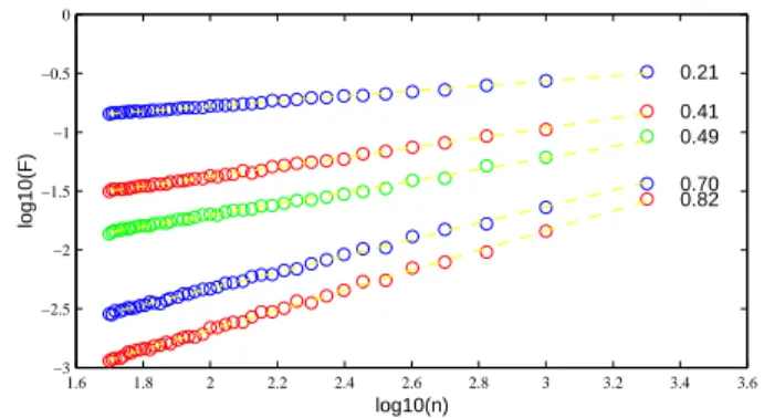
On the right side of Figure 2 appear the different estimations
of H computed from the DFA method. Those values have to
be compared with theoretical ones. The results seem to be quite good and it seems that, under certain conditions, the asymptotic behavior of the DFA functionF (n) can be written as
F (n)' c(σ, H) · nH (7)
where c is a positive function depending only on σ and H (see its expression above).
1.6 1.8 2 2.2 2.4 2.6 2.8 3 3.2 3.4 3.6 −3 −2.5 −2 −1.5 −1 −0.5 0 log10(n) log10(F) 0.21 0.41 0.49 0.70 0.82
Fig. 2. Results of the DFA method applied to a path of a discretized FGN for different values ofH = (0.2, 0.4, 0.5, 0.7, 0.8) (also with N = 10000)
The approximation (7) explains that the slope of the least-square regression line of(log F (ni)) by log(ni) for different
values of ni provides an estimation ofH. We now provide a
mathematical proof of this result.
Let {XH(t), t ≥ 0} be a FBM, built as a cumulated
sum of a FGN {YH(t), t ≥ 0}. We £rst give some asymptotic properties ofF2
Property 3.1: Let{XH(t), t≥ 0} be a FBM with param-eters0 < H < 1 and σ2> 0. Then, for n and j large enough,
1. (F2 1(n)) = σ2f (H)· n2H ³ 1 + O¡ 1 n ¢´ , 2. Var¡F2 1(n) ¢ = σ4g(H)· n4H³1 + O¡ 1 n ¢´ , 3. Cov(F2 1(n), Fj2(n)) = σ4h(H)³ · n4H· j2H−3· 1 + O¡ 1 n ¢ + O¡ 1 j ¢´ , with f (H) = (1− H) (2H + 1)(H + 1)(H + 2) , g depending only on H, see (20), and h(H) = H 2(H − 1)(2H − 1)2 48(H + 1)(2H + 1)(2H + 3).
The proofs of these results (and of the others) are provided in Appendix I.
In order to obtain a central limit theorem for the logarithm of the DFA function, we consider normalized DFA functions
˜ Sj(n) = F2 j(n) n2Hσ2f (H) and S(n) =˜ F2(n) n2Hσ2f (H) (8) for n∈ {1, . . . , N} and j ∈ {1, . . . , [N/n]}.
As a consequence, for n ∈ {1, . . . , N}, the stationary time series ( ˜Sj(n))1≤j≤[N/n] satisfy ( ˜Sj(n)) = 1 + O ¡ 1 n ¢ Var( ˜Sj(n)) = g(H) f (H)2 ³ 1 + O¡ 1 n ¢´ Cov( ˜S1(n), ˜Sj(n)) = h(H) f (H)2 · 1 j3−2H· ³ 1 + O¡ 1 n ¢ + O¡ 1 j ¢´ (9)
Under certain conditions on the asymptotic length n of the windows, one proves a central limit theorem satis£ed by the logarithm of the empirical mean ˜S(n) of the random variables ( ˜Sj(n))1≤j≤[N/n].
Property 3.2: Under the previous assumptions and
nota-tions, let n ∈ {1, . . . , N} be such that N/n → ∞ and
N/n3 → 0 when N → ∞. Then r £ N n ¤ · log( ˜S(n)) −→L n→∞ N →∞ N (0, γ2(H))),
where γ2(H) > 0 depends only on H.
This result can be obtained for different lengths of windows satisfying the conditions N/n → ∞ and N/n3 → 0. Let
(n1, . . . , nm) be such different window lengths. Then, one can
write for N and ni large enough
log( ˜S(ni))' 1 p [N/ni]· ε i =⇒ log(F (ni))' H · log(ni) + 1 2 log(σ 2f (H)) + 1 p [N/ni]· ε i,
withεi∼ N (0, γ2(H)). As a consequence, a linear regression
of log(F (ni)) on log(ni) provides an estimation of H. More
precisely,
Proposition 3.3: Under the previous assumptions and
nota-tions, letn∈ {1, . . . , N}, m ∈ ∗
\ {1}, ri∈ {1, . . . , [N/n]}
for each i with r1 < · · · < rm and ni = rin be such that
N/n → ∞ and N/n3
→ 0 when N → ∞. Let bH be the
estimator of H from the linear regression of log(F (ri· n))
on log(ri· n), i.e.
b H =
Pm
i=1(log(F (ri· n)) − log(F ))(log(ri· n) − log(n))
Pm
i=1(log(ri· n) − log(n))2
. Then bH is a consistant estimator of H such that
[( bH− H)2]≤ C(H, m, r1, . . . , rm)
1
[N/n] (10)
withC(H, m) > 0.
IV. EXTENSION OF THE RESULTS FOR A GENERAL CLASS OF A LONG-RANGE DEPENDENT PROCESS
Let {Y (k), k ∈ } be a stationary zero mean long-range
dependent process with a Hurst parameter H ∈]12, 1[. More precisely, let rY(k) be the autocorrelation function of this
process and let us assume that there exists a slowly varying functionL(k) such that:
rY(k)∼ k2H−2L(k) , as k→ ∞. (11)
Under different additional assumptions on Y , Davydov [9], Taqqu [32], Dobrushin and Major [11], Giraitis and Surgailis [15] and other authors have studied the asymptotic behavior of the Donsker line and obtained the following convergence,
¡ L(n)−12n−H [nt] X i=1 Y (i)¢t>0 −→D n→∞ ¡ σ· BH(t) ¢ t>0, (12)
with σ > 0 and BH a fractional Brownian motion. Remind
that Z ={Z(k), k ∈ } is a linear process when
Z(k) =
∞
X
i=−∞
aiξk−i for k∈ ,
with(ak) a sequence of real numbers and (ξn) a sequence of
zero mean i.i.d.r.v. Then,
Theorem 4.1: (Davydov, Taqqu) Let Y = {Y (k), k ∈ } be a stationary zero mean long-range dependent process satisfying assumption (11). Then, if:
• Y is a linear process,
• or Y is a function of a Gaussian process with Hermite
rankr = 1,
then (12) holds, and the convergence takes place in the Skorohod space.
Limit theorems are also obtained by Dobrushin and Major [11], Giraitis and Surgailis [15] and Ho and Hsing [16] for sums of polynomials of linear (or moving average) process with slowly decreasing coef£cientsai. It is obtained under the
hypothesis that(ξn) are i.i.d standard normal random variable
So, in this case of general class of LRD process, the aggregated process (X(k)) has roughly the same behavior as a fractional Brownian motion and the previous asymptotic results of the DFA method can be applied. But Property 3.1 and Proposition 3.3 cannot be proved under so general assumptions. Indeed, the proofs of such results use a very precise expression of the covariance and a stronger version of assumption (11) is necessary. Hence, the covariance rY
of the stationary process Y is now supposed to satisfy
rY ∈ H(H, β, C) with
H(H, β, C) =nr, r(k) = C· k2H−2¡1 + O(1/kβ)¢
when k→ ∞o, (13)
with 1/2 < H < 1, C > 0 and β > 0. In such a
semi-parametric frame, the previous proofs are still valid and :
Theorem 4.2: Let Y = {Y (k), k ∈ } be a Gaussian stationary zero mean long-range dependent process with co-variance rY ∈ H(H, β, C). Then, Property 3.1 holds with
the addition of O(1/nβ) in each expansion. Moreover, if
N = o¡nmax(2β+1,3)¢, Property 3.2 and Proposition 3.3 hold.
As a consequence of this theorem, if 0 < β ≤ 1, the DFA method provides a semi-parametric estimator of H with the well-known minimax rate of convergence for the estimation of Hurst parameter in this semi-parametric setting (see for instance Giraitis et al. [13]), i.e.
lim sup
N →∞
sup
rY∈H(H,β,C)
N2β/(1+2β) [( bH− H)2] < +∞. However, if β ≥ 1, this result is replaced with lim sup N →∞ sup rY∈H(H,β,C) N2/3 [( bH− H)2] < + ∞ (β = 2 for instance for FGN or Gaussian FARIMA(p, d, q)). Thus, the DFA estimator is not rate optimal for all β > 0 like local Whittle, local log-periodogram or wavelet based estimators are (see respectively [29], [14] and [24]).
V. CASES OF PARTICULAR TRENDED LONG-RANGE DEPENDENT PROCESSES
In this Section, two general examples of trended long-range dependent processes are considered and it is proved that the DFA method in such cases yields a biased and unusable estimation of the Hurst parameter.
In order to consider trended processes, the following lemma for two independent processes could be considered :
Lemma 5.1: Let Y = {Y (k), k ∈ } and Y0 =
{Y0(k), k
∈ } be two independent processes, with
(Y (k)) = 0 for all k ∈ , and let us denote respectively
F2
Y, FY20 andFY +Y2 0 the DFA functions associated to Y , Y0
andY + Y0. Then, forn
∈ {1, · · · , N},
(FY +Y2 0(n)) = (FY2(n)) + (FY20(n)).
Proof: WithX and X0 the aggregated processes associated to
Y and Y0, it is obvious that
(FY +Y2 0(n)) = 1 n· [N/n] n·[N/n]X k=1 ³³ X(k) + X0(k) − bXn(k)− bXn0(k) ´2´ = (FY2(n)) + (FY20(n)) + 2 n· [N/n]· n·[N/n] X k=1 ³¡ X(k)− bXn(k)¢¡X0(k)− bXn0(k) ¢´ . From the independence of X and X0 and thanks to the
assumption (Y (k)) = 0 for all k ∈ which implies
(X(k)) = 0 and ( bX(k)) = 0 for all k∈ , we deduce
³¡ X(k)− bXn(k) ¢¡ X0(k) − bX0 n(k) ¢´ = 0. ¤
Let Y = {Y (k), k ∈ } be a Gaussian stationary zero
mean long-range dependent process satisfying assumption (13) (for instance, Y is a FGN) and let f : 7→ be a deterministic function. From Lemma 5.1, it is obvious that for n∈ {1, · · · , N},
(FY +f2 (n)) = (FY2(n)) + (Ff2(n)). (14)
Moreover, let us denote respectively F2
Y,j and Ff,j2 the DFA
function of Y and f relating to window j ∈ {1, . . . , [N n]}.
Then, with few changes in the proof of Lemma 5.1, (F2
Y +f,j(n)) = (FY,j2 (n)) + (Ff,j2 (n)). (15)
Case of power law and polynomial trends
First, let us assume that there existsλ > 0 and a∈ such that
f (t) = a(tλ+1− (t − 1)λ+1), for t≥ 1.
Then, the associated integrated function is g(k) =
k
X
i=1
f (i) = akλ+1.
For this kind of trend,
Property 5.1: For f (t) = a(tλ+1
− (t − 1)λ+1), with
γ(a, N, λ) a real number depending only on a, N and λ,
log Ff(n)' 2 log n + γ(a, N, λ) for n → ∞.
Thus, it appears that a linear regression of log Ff(ni) and
log(ni) for different values of ni will provide a slope 2 for
any λ > 0. This result is con£rmed by several simulations
made for various values of λ > 0, a and (n1, . . . , nm).
This result can also be used to deduce similar results for polynomial trends.
Property 5.2: Let us assume that there exists p ∈
∗ and a family (a
j)0≤j≤p with ap 6= 0 such that
for k ∈ , f (k) = apkp + · · · + a0. Then,
Using relations (14) and (15), the previous results for trends can be used for deducing the behavior of the DFA function of trended long range dependent processes. Hence, in both previous cases of trends, there exists C > 0 such that
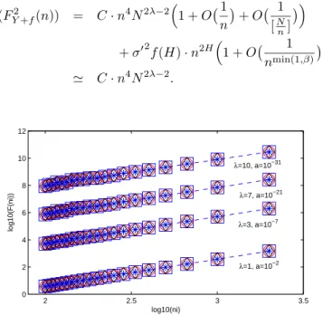
(F2 Y +f(n)) = C· n4N2λ−2 ³ 1 + O¡ 1 n ¢ + O¡ 1 [Nn] ¢´ + σ02f (H)· n2H³1 + O¡ 1 nmin(1,β) ¢´ ' C · n4N2λ−2. 2 2.5 3 3.5 0 2 4 6 8 10 12 log10(ni) log10(F(ni)) λ=10, a=10−31 λ=7, a=10−21 λ=3, a=10−7 λ=1, a=10−2
Fig. 3. Relation betweenlog FY +f(ni) and log niin the case of a power
law trend (N = 10000, H = 0.2 (¤), H = 0.4 (°), H = 0.5 (♦),
H = 0.7 (∗) and H = 0.8 (·))
Thus, it is clear that the trend is dominant for a large n and the graph exhibiting the relation between log FY +f(ni) and
log ni for different power law trends and different coef£cients
H con£rms this (the estimated slope is always close to 2).
Case of a piecewise constant trend
Let us assume now that f is a step function of the form f (t) =
m−1X i=0
ai ]ti,ti+1] with t0 = 0, tm = N and m ∈
∗.
The associated integrated series is g(k) = m−1X i=0 ¡Xi s=0 (as−1− as)ts+ aik¢ ]ti,ti+1] witha−1 = 0.
For j ∈ {1, . . . , [N/n]}, the partial DFA function F2
f j(n) is
null unless there exist ip with p ∈ {1, . . . , r} and (r, ir) ∈
{1, . . . , m − 1}2 such that t
ip ∈ [(jp− 1)n + τn, jpn− τn]
with τ ∈]0,12[. In such a case, we calculate the partial DFA
function: Ff,j2 p(n) = 1 n n X k=1 (g(k + (jp− 1)n) − bgn(k + (jp− 1)n))2 = 1 n ³ G(jp)0· P E⊥ jp · G (jp) ´ .
If we consider the £rst window, the partial DFA function can be estimated from below :
Ff,12 (n)≥ 1 n ³Xτ n k=1 (g(k)− bgn(k))2+ n X k=n−τ n (g(k)− bgn(k))2 ´
where the n× 1 vector ¡g(k)− bgn(k)
¢ 1≤k≤n = PE⊥1 · G (1) with : G(1)=¡a0· 1, . . . , a0· t1, (a0− a1)t1+ a1· (t1+ 1), . . . , (a0− a1)t1+ a1· n¢ 0 . Then, τ n X k=1 (g(k)− bgn(k))2= ³ Jτ n· PE⊥ 1 · G (1)´0 ·³Jτ n· PE⊥ 1 · G (1)´
where Jτ n is a square matrix of order n with ones in the
τ n £rst terms of the diagonal and zeros elsewhere. When we approximate sums by integrals, this expression can be written as follows : τ n X k=1 (g(k)− bgn(k))2= n3 ³ Z τ 0 ³ Z 1 0 a0y−¡a0x· x≤t1 n+ ¡ a1x + (a0− a1) t1 n ¢ x>t1n ¢ (4− 6(x + y) + 12xy)dx´2dy´· ³ 1 + O¡ 1 n ¢´ . For τ ∈]0,1
2[, the second term can be developed in the same
way by replacingJτ nbyJn−τ nwhich isId−Jτ n. Then, this
term can be approximated by :
n X k=n−τ n (g(k)− bgn(k))2= n3 ³ Z 1 1−τ ³ Z 1 0 (a0− a1)t1 n + a1y −¡a0x· x≤t1 n + ¡ a1x + (a0− a1) t1 n ¢ x>t1n ¢ (4− 6(x + y) + 12xy)dx´2dy´³1 + O¡ 1 n ¢´ . Then after developing the two terms, we deduce that there exists a positive number c(a0, . . . , aip, tip, τ ) such that the
partial DFA function in thejp-th window, wheretip∈ [(jp−
1)n + τ n, jpn− τn] for p ∈ {1, . . . , r} and n large enough,
can be written as :
Ff,j2 p(n)≥ c(a0, . . . , aip, tip, τ )n
2. (16)
Then if we suppose that there exists only one change point or a de£nite number of windows j1, . . . , jr, there exists
c0(a
0, . . . , air, ti1, . . . , tir, τ ) > 0 such that the DFA function
relating to f is : Ff2(n) = 1 [Nn] jr X j=j1 F2f,j(n)≥ c0(a0, . . . , air, ti1, . . . , tir, τ )n 3N−1³1 + O¡ 1 n ¢´ . If we consider the signal formed by the superposition between the trend and a long range dependent process, we point out that (F2 Y(n)) = σ02f (H)· n2H ³ 1 + O¡ 1 nmin(1,β) ¢´ . We can deduce, from the previous conditions onn and N (N/n→ ∞
andN = o(nmin(3,2β+1)), that the trend is dominant for large
n.
Then, for different values(n1, . . . , nm), the graph tracing the
relation betweenlog Ff +Y(ni) and log(ni) (Figure 4), shows
2 2.2 2.4 2.6 2.8 3 −1 −0.5 0 0.5 1 1.5 2 2.5 3 log10(ni) log10(F(ni)) 60 Change−pts 20 Change−pts 5 Change−pts
Fig. 4. Relation betweenlog Ff +Y(ni) and log niin the case of a trend
with change points (N = 20000, H = 0.2 (¤), H = 0.4 (°), H = 0.5
(♦),H = 0.7 (∗) and H = 0.8 (·))
VI. CONCLUSION
In the semi-parametric frame of a long-memory stationary process, we have shown, using the DFA method, that the estimator of the long range dependence parameter is convergent with a reasonable (but not always optimal) convergence rate. However, in numerous cases of trended long-range dependent process (with perhaps the only exception of a constant trend), this estimator does not converge. Indeed the effect of long-memory property is dominated by the effect of the trend in the case of power law or polynomial trends. The slope for the trended processes of the DFA log-log regression is always close to 2 and in the case of a piecewise constant trend, the slope is estimated at
3
2. The DFA method is therefore not robust at all and should
not be applied for trended processes.
The wavelet-based method provides a more ef£cient and robust estimator of the Hurst parameter especially when a polynomial trended LRD (or self-similar) process is considered. Indeed, Abry et al. [1] remarked that all polynomial trend of degree M is without effects on the estimator of the Hurst parameter as soon as the mother wavelet has its M £rst vanishing moments. Therefore, the larger M , the more robust the estimator is. Moreover, in the semi-parametric frame of general class of stationary Gaussian LRD processes, it was established by Moulines et al. [24] that the estimator of the Hurst parameter converges with an optimal convergence rate (following the minimax criteria) when an optimal length of windows is known. Bardet et al. [6] proposed an adaptive estimator and obtained an optimal convergence rate up to logarithmic factor. Finally, the wavelet based estimator can be computed by Mallat’s fast cascade algorithm which is a very fast algorithm (the equivalent for wavelet transform of FFT for Fourier transform) for computing wavelet coef£cients. Thus, computing time of wavelet based estimator is smaller than DFA estimator one.
APPENDIXI
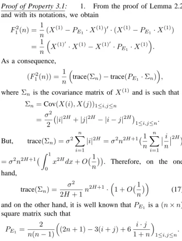
Proof of Property 3.1: 1. From the proof of Lemma 2.2 and with its notations, we obtain
F12(n) = 1 n(X (1) − PE1· X (1))0 · (X(1)− PE1· X (1)) = 1 n ³ X(1)0 · X(1) − X(1)0 · PE1· X (1)´. As a consequence, (F12(n)) = 1 n ³ trace(Σn)− trace(PE1· Σn) ´ , where Σn is the covariance matrix ofX(1) and is such that
Σn= Cov(X(i), X(j))1≤i,j≤n = σ 2 2 ¡ |i|2H+ |j|2H − |i − j|2H¢ 1≤i,j≤n. But, trace(Σn) = σ2 n X i=1 |i|2H= σ2n2H+1¡ 1 n n X i=1 ¯ ¯i n ¯ ¯2H¢ = σ2n2H+1¡ Z 1 0 x2Hdx + O¡ 1 n ¢¢
. Therefore, on the one hand, trace(Σn) = σ 2 2H + 1n 2H+1 ·³1 + O¡ 1 n ¢´ (17) and on the other hand, it is well known thatPE1 is a(n× n)
square matrix such that
PE1= 2 n(n− 1) ³ (2n + 1)− 3(i + j) + 6 i· j 1 + n ´ 1≤i,j≤n.
Then, after some straightforward computations, we obtain the formula trace(PE1· Σn) = σ2n2H+1n2 n(n− 1) n X p=1 n X q=1 h 1 n2 ³ (2 + 1 n)− 3· p + q n + 6p· q n(1 + n) ´³¯¯q n ¯ ¯2H +¯¯p n ¯ ¯2H −¯¯q− pn ¯¯2H´i. In order to clarify the formula, we approximate these sums by integrals trace(PE1· Σn) = σ 2n2H+1 ·³1 + O¡ 1 n ¢´ · Z 1 0 Z 1 0 h¡
2− 3(x + y) + 6xy)¢¡x2H+ y2H− |x − y|2H¢idxdy.
After the calculation of this integral and a simpli£cation with formula (17), we get the result
trace(Σn)− trace(PE1· Σn) = σ
2f (H)
· n2H+1·³1 + O¡ 1
n ¢´ and therefore the formula of (F2
1(n)).
2. From the previous notations and the property of the trace of a product of matrices,
Var(F12(n)) = 1 n2 h (X(1)0· PE⊥ 1 · X (1) · X(1)0 · PE⊥ 1 · X (1)) −³ (X(1)0· PE⊥ 1 · X (1))´2i = 1 n2 h trace(Σn· Σn)− trace(PE1· Σn· Σn) i (18)
The development of the £rst term provides the following asymptotic expansion trace(Σn· Σn) = σ4 4 n X i=1 n X p=1 ¡ |i|2H+ |p|2H − |i − p|2H¢2= σ4 4 n 4H+2³1 + O¡ 1 n ¢´Z 1 0 Z 1 0 ¡ |x|2H+ |y|2H − |x − y|2H¢2dxdy.
The calculation of this integral provides the following simpli-£ed expression trace(Σn· Σn) = σ4 4 n 4H+2³1 + O¡ 1 n ¢´ · h 1 4H + 1+ 1 (4H + 1)(4H + 2)− 2 (Γ(2H + 1))2 Γ(4H + 3) i . (19)
The same development can be made for the second term trace(PE1· Σn· Σn) = σ4 2 n 4H+2³1 + O¡ 1 n ¢´ · Z 1 0 Z 1 0 Z 1 0 ³ |x|2H+ |y|2H − |y − x|2H´³ |x|2H+ |z|2H − |x − z|2H´ ·³2− 3(y + z) + 6yz´dx dy dz.
After the computation of this last integral, and using relations (18) and (19) h trace(Σn· Σn)− trace(PE1· Σn· Σn) i = σ4· g(H) n4H+2³1 + O¡ 1 n ¢´ , withg(H) = 1 2 ³ −(16H 2+ 24H + 17)(Γ(2H + 1))2 (4H + 5)Γ(4H + 4) (20) + H + 1 (2H + 1)(4H + 1)+ 7H + 3 2(2H + 1)2(H + 1)− 3 2(H + 1)2 + 3(4H + 3) 2(2H + 1)2(H + 1)2(4H + 5)− 4 (2H + 1)2(4H + 3) ´ .
Then, using the relations (18), we obtain
Var¡F12(n) ¢ = σ4· g(H) · n4H³1 + O¡ 1 n ¢´ .
3. An asymptotic expansion of the covariance between two DFA functions in two suf£ciently far windows can be provided. Indeed, Cov(F12(n), Fj2(n)) = 1 n2· Cov³¡X(1)− bX(1)¢0¡X(1)− bX(1)¢¡X(j)− bX(j)¢0¡X(j)− bX(j)¢´ = 1 n2 ³ trace ³ Σ(1,j)· Σ(1,j)´− trace³PE1· Σ (1,j) · Σ(1,j)´´, because PE⊥ 1 = PEj⊥ and with Σ
(1,j) the covariance matrix
(X(1)·X(j),) = (σ(1,j)
k,k0 )1≤k,k0≤n. As usual, this formula can
be developed by Cov(F12(n), Fj2(n)) = 1 n2 ³Xn k=1 n X k0=1 σk,k(1,j)0 · σ (1,j) k0,k − n X i=1 n X k0=1 n X k=1 pi,k· σ(1,j)k,k0 · σ (1,j) k0,i ´ , with σ(1,j)k,k0 = σ2 2 ¡ |k + nj|2H+|k0|2H− |k − k0+ nj|2H¢1≤k,k0≤n
and with PE1 = (pi,j)1≤i,j≤n such that
pi,j= 2
n(n− 1)
³
(2n + 1)− 3(i + j) + 61 + ni· j ´. Now, we consider the asymptotic expansion of this formula
when n is large enough
Cov(F12(n), Fj2(n)) = σ4 4 n 4H³1 + O¡ 1 n ¢´³ Z 1 0 Z 1 0 ¡ |x+j|2H + y2H− |x − y + j|2H¢¡|y + j|2H+ x2H− |y − x + j|2H¢dxdy − Z 1 0 Z 1 0 Z 1 0 (4− 6(x + z) + 12xz)¡|x + j|2H+ y2H− |x − y + j|2H¢ ¡ |y+j|2H+z2H −|y−z+j|2H¢dx dy dz´.
In order to obtain an asymptotic expansion of this formula
when j is large enough (i.e. both windows are taken away
from one another), a Taylor expansion in j up to order 3 is necessary. After calculating and simplifying the integrals, we
get the result. ¤
Proof of Property 3.2: We divide the proof into3 steps:
• Step 1: one proves that [N/n] · Var( ˜S(n)) → γ2(H),
whereγ2(H) depends only on H, when [N/n]→ ∞. Indeed,
Var( ˜S(n)) = 1 [Nn]2 [N n] X j=1 [N n] X j0=1 Cov( ˜Sj(n), ˜Sj0(n)) = 1 [N n] Var( ˜Sj(n)) + 2 [N n]2 [N n] X j=1 ¡ [N n]− j ¢ Cov( ˜S1(n), ˜Sj(n))
due to the stationarity.
However, with properties (9), one deduces that when[N/n]→ ∞, [N n] X j=1 Cov( ˜S1(n), ˜Sj(n)) and [N n] X j=1 j· Cov( ˜S1(n), ˜Sj(n))
converge, because there exists C ≥ 0 such that ¯
¯Cov( ˜S1(n), ˜Sj(n))
¯
¯ ≤ C · j2H−3 and0 < H < 1.
Therefore, there exists γ2(H) depending only on H
such that lim
[N/n]→∞[N/n]· Var( ˜S(n)) = γ
2(H). (21)
• Step 2: the proof of a central limit theorem for ˜S(n) when
[N/n]→ ∞ can be obtained from the same method as in the
proof of Proposition 2.1 in Bardet [4] (Theorem 3 in Soulier [31] leads to the same result).
Indeed, ˜S(n) = 1
n2H+1σ2f (H)· [N/n]
n·[N/n]X i=1
Zi2, where the
zero-mean Gaussian vector Z = (Z1, . . . , Zn·[N/n]) has the
covariance matrix P · Σ · P , where P is a diagonal block matrix with each block consisting of (n, n) matrix PE⊥
1 and
block isΣ(i,j)with the previous notations). Using a Lindeberg
condition, ˜S(n) satis£es the following central limit theorem : p
[N/n]·³S(n)˜ − (S(n))´ −→L
[N/n]→∞ N (0, γ
2(H))), (22)
if λ = kP · Σ · P k, the supremum of the eigenvalues of the
symmetrical matrix P· Σ · P , is such that
λ = o³p 1
[N/n] ´
. (23)
But, using Lemma 4.1 and following the proof of Proposition 2.1 in Bardet [4], λ ≤ 1 n2H+1σ2f (H)· [N/n]· max i∈{1,...,n·[N/n]} n·[N/n]X j=1 |Cov¡Zi, Zj)| λ ≤ √ 1 2[N/n] i∈{1,...,n·[N/n]}max n·[N/n]X j=1 q |Cov¡Z2 i, Zj2)| n2H+1σ2f (H) ≤ √ 1 2[N/n] i∈{1,...,[N/n]}max [N/n]X j=1 q Cov¡ ˜Si(n), ˜Sj(n) ¢ ≤ √ 2 [N/n] [N/n] X j=1 q Cov¡ ˜S1(n), ˜Sj(n)¢ .
So, there existsC(H) > 0 depending only on H such that
λ ≤ C(H) · 1 [N/n] [N/n]X j=1 ³p j2H−3+ c n ´ third line of (9) ≤ C0(H) ·³[N/n]H−3/2+1 n ´ . (24) Therefore if n1 = o³√ 1 [N/n] ´
(i.e.N = o(n3)), (23) and (22)
are proved.
• Step 3: Now, ( ˜S(n)´= 1 + O¡ 1
n ¢
for n large enough.
Then, ifp[N/n]· 1 n → 0, that is N/n 3 → 0, p [N/n]·³S(n)˜ − 1´ −→L [N/n]→∞ N (0, γ 2(H))).
The classical Delta method allows the passage between a central limit theorem for ˜S(n) and a central limit theorem for
log( ˜S(n)) (thanks to the regularity properties of the function
logarithm). ¤
Proof of Proposition 3.3: It is possible to write b
H = (1, 0)· (Z0
· Z)−1
· Z0
· F , where Z is the (m, 2)
matrix such that Z =
log(r1· n) 1 .. . ... log(rm· n) 1 and F = log(F (r1· n)) .. . log(F (rm· n)) . Then Var( bH) = (1, 0)· (Z0· Z)−1· Z0· Cov(F, F ) · Z · (Z0· Z)−1· (1, 0)0 ≤ k(1, 0) · (Z0· Z)−1· Z0k2· kCov(F, F )k ≤ k(1, 0) · (Z0 · Z)−1 · Z0 k2 · 2m · m Y i=1 ri· γ2(H)· 1 [N/n].
Since k(1, 0) · (Z0· Z)−1· Z0k only depends on r1, . . . , rm,
the proof of Proposition 3.3 is completed. ¤
Proof of Theorem 4.2: From the assumptions on Y and rY, ifi≥ j ≥ 1, Cov(X(i), X(j)) = i X k=1 j X `=1 Cov(Y (k), Y (`)) = i X k=1 (i− k)rY(k) + j X k=1 (j− k)rY(k)− i−j X k=1 (i− j − k)rY(k).
As a consequence, for all (i, j)∈ {1, . . . , n}2,
Cov(X(i), X(j)) = C·³ Z 1 0 (1− u)u2H−2du´· ³ i2H¡1 + O¡ 1 imin(β,1) ¢¢ + j2H¡1 + O¡ 1 jmin(β,1) ¢¢ − |i − j|2H¡1 + O¡ 1 (1 +|i − j|)min(β,1) ¢¢´ · Now, this covariance can be used for the proofs replacing the previous ones. This implies
1. (F2 1(n)) = σ02f (H)· n2H ³ 1 + O¡ 1 nmin(β,1) ¢´ , 2. Var¡F2 1(n) ¢ = σ04g(H) · n4H³1 + O¡ 1 nmin(β,1) ¢´ , 3. Cov(F2 1(n), Fj2(n)) = σ04h(H)³ · n4H· j2H−3· 1 + O¡ 1 nmin(β,1) ¢ + O¡ 1 j ¢´ , withσ02= 2C·³ Z 1 0
(1− u)u2H−2du´. The proofs of
prop-erty 3.2 are the same as in the case of the FGN except that in (24), λ ≤ C(H) · 1 [N/n] [N/n]X j=1 ³p j2H−3+ c n+ c nβ ´ ≤ C0(H) ·³[N/n]H−3/2+ 1 n+ 1 nβ ´ . So, if n1+ 1 nβ = o ³ 1 √ [N/n] ´ thereforeN = o¡nmax(2β+1,3)¢,
the central limit theorem as well as Proposition 3.3 are proved following the same proof as in the case of the FGN. ¤
Proof of Property 5.1: In the j-th window, with
subspace de£ned above and de£ne the vector G(j)= a((1 + n(j − 1))λ+1, . . . , (nj)λ+1)0. We have F2 f,j(n) = 1 n ³ G(j)0 · G(j) − G(j)0 · PEj · G (j)´
An explicit asymptotic expansion (in n and N ) of this partial DFA function can be obtained by approximating sums by integrals. Then, Ff,j2 (n) = a2n2λ+2 ³ 1 + O¡ 1 n ¢´³ Z 1 0 Z 1 0 (x + j− 1)2λ+2 − (4− 6(x + y) + 12xy)(x + j − 1)λ+1(y + j− 1)λ+1dxdy´
Moreover, using Taylor expansion in j up to order 3, one obtains Ff,j2 (n) = α(a, λ)· n2λ+2j2λ−2 ³ 1 + O¡ 1 n ¢ + O¡ 1 j ¢´ , (25) and it implies that the DFA function relating to f can be written as Ff2(n) = 1 [N/n] [N/n] X j=1 Ff,j2 (n) = β(a, λ)· n4N2λ−2³1 + O¡ 1 n ¢ + O¡ 1 [Nn] ¢´ ,
with α(a, λ), β(a, λ) two positive numbers depending only
on a and λ. ¤
Proof of Property 5.2: Letf (k) = apkp+· · · + a0 =⇒
g(k) =
k
X
i=1
f (i) = bp+1kp+1+· · · + b0, with bp+1 6= 0,
i.e. the associated integrated function is also a polynomial
function. From the expression of the partial DFA function and with the asymptotic expansion (25) depending on the degreeλ, for n and N large enough,
Fa2pkp+···+a0,j(n) = F 2 apkp,j(n) ³ 1 + O¡ 1 n ¢ + O¡ 1 j ¢´ (the power of n in the partial DFA function relating to apkp
is greater than the ones in the partial DFA function relating to the other monomes). This approximation leads to the following expression of the DFA function of a polynomial function,
Fa2pkp+···+a0(n) = β(bp+1)· n4N2λ−2 ³ 1 + O¡ 1 n ¢ + O¡ 1 [N n] ¢´ . ¤ ACKNOWLEDGMENT
We would like to thank a lot Véronique Billat, Professor at the Université d’Evry Val d’Essonne, France, for presenting this subject to us and providing us with numerous articles and data on this topic.
REFERENCES
[1] Abry P., Veitch D., Flandrin P., Long-range dependence: revisiting
aggregation with wavelets., J. Time Ser. Anal. 19, no. 3, 253-266, 1998.
[2] Absil P.A., Sepulchre R., Bilge A., Gérard P., Nonlinear analysis of
cardiac rhythm ¤uctuations using DFA method, J. Physica A : Statistical
mechanics and its applications, 235-244, 1999.
[3] Arcones M., Limit theorems for nonlinear functionals of a stationary
Gaussian sequence of vectors., Ann. Probab. 22, 2242-2274, 1994.
[4] Bardet J.M., Testing for the presence of self-similarity of Gaussian time
series having stationary increments, J. of Time Series Anal. 21, 497-516,
2000.
[5] Bardet J.M., Statistical study of the wavelet analysis of fractional
Brow-nian motion, IEEE Trans. Inform. Theory. 48, 991-999, 2002.
[6] Bardet J.M., Bibi H., Jouini A. Adaptive wavelet based estimator of the
memory parameter for stationary Gaussian processes, Preprint of Samos,
University Paris 1, 2006.
[7] Bardet J.M., Lang G., Oppenheim G., Philippe A., Taqqu M.S. Generators
of long-range dependent processes : A survey. In Long-range Dependence : Theory and Applications, Birkhauser (2002).
[8] Chen Z., Ivanov P.C., Hu K., Stanley H.E, Effect of nonstationarities on
detrended ¤uctuation analysis, Physical Review E, Vol. 65, 041107, 2002.
[9] Davydov Y.A., The invariance principal for stationry processes, Theory Probab. Appl. 15, 487-498, 1970.
[10] Delignières D., L’analyse des processus stochastiques, "Sport, Perfor-mance, Santé", EA 2991, Université Montpellier I, janvier 2001. [11] Dobrushin R.L., Major P., Non-central limit theorems for nonlinear
functionals of Gaussian £elds, Z. Wahrsch. Verw. Gebiete 50, 27-52,
1979.
[12] Gao J.B., Cao Y., Lee J.M, Principal component analysis of1/fαnoise, Physics Letters, A 314, 392-400, 2003.
[13] Giraitis L., Robinson, P. and Samarov, A., Rate optimal semi-parametric
estimation of the memory parameter of the Gaussian time series with long range dependence, J. Time Ser. Anal., 18, 49-61, 1997.
[14] Giraitis L., Robinson, P. and Samarov, A., Adaptive Semiparametric
Estimation of the Memory Parameter, Journal of Multivariate Analysis,
Vol. 72, Issue 2, 183-207, 2000.
[15] Giraitis L., Surgailis D., CLT and other limit theorems for functionals
of Gaussian processes, Z. Wahrsch. Verw. Gebiete 70, 191-212, 1985.
[16] Ho H.C., Hsing T., Limit theorems for functionals of moving averages, The Annals of Probability, Vol. 25, No. 4, 1636-1669, 1997.
[17] Hu K., Ivanov P.C., Chen Z., Carpena P., Stanley H.E, Effect of trends
on detrended ¤uctuation analysis, Physical Review E, Vol. 64, 011114,
2001.
[18] Hwa R.C., Ferree T.C.,Fluctuation analysis of human
electroencephalo-gram, Nonlinear phenomena in complex systems, 302-307, 2002.
[19] Kantelhardt J.W., Ashkenazy Y., Ivanov P.C., Bunde A., Havlin S., Penzel T., Peter J.H., Stanley H.E., Characterization of sleep stages by
correlations in the magnitude and sign of heartbeat increments, Physical
Review E, Vol. 65, 051908, 2002.
[20] Kantelhardt J.W., Koscielny-Bunde E., Rego H.A.H., Havlin S., Bunde A., Detecting Long- range Correlations with Detrended Fluctuation
Analysis, Physica A, 295, 441-454, 2001.
[21] Karasik R., Sapir N., Ashkenazy Y., Ivanov P.C., Dvir I., Lavie P., Havlin S., Correlation differences in heartbeat ¤uctuations during rest
and exercise, Physical Review E 66, 062902, 2002.
[22] Martinis M., Knezevic A., Krstacic G., Vargovic E., Changes in the
Hurst exponent of heartbeat intervals during physical activities, Physics
0212029, 2002.
[23] Masugi M., Detrended ¤uctuation analysis of IP-network traf£c using a
two-dimensional topology map, Phys. A 337, no. 3-4, 664–678, 2004.
[24] Moulines E., Roueff F., Taqqu M.S., On the Spectral Density of the
Wavelet Coef£cients of Long-Memory Time Series with Application to the Log-Regression Estimation of the Memory Parameter, JTSA, Vol. 28,
issue 2, 155-187, 2007.
[25] Nagarajan R., Kavasseri R.G, Minimizing the effect of sinusoidal trends
in detrended ¤uctuation analysis, (in press) International Journal of
Bifurcations and Chaos, Vol. 15, No. 2, 2005.
[26] Peng C.K., Buldyrev S.V., Havlin S., Simons M., Stanley H.E., Gold-berger A.L., Mosaic organization of DNA nucleotides, Physical Review E, Vol. 49, 1685-1689, 1994.
[27] Peng C.K., Hausdorff J.M., Goldberger A.L., Fractal mechanisms in
neural control: Human heartbeat and gait dynamics in health and disease. In: Walleczek J, ed. Nonlinear Dynamics, Self-Organization, and
[28] Peng C.K., Havlin S., Stanley H.E., Goldberger A.L., Quanti£cation of
scaling exponents and crossover phenomena in nonstationary heartbeat time series, Chaos 5, 82, 1995.
[29] Robinson, P.M.Gaussian semiparametric estimation of long range
de-pendence, The Annals of statistics, 23:1630-1661, 1995.
[30] Samorodnitsky G., Taqqu M.S., Stable non-Gaussian Random Processes, Chapman and Hall, 1994.
[31] Soulier P., Moment bounds and central limit theorem for functions of
Gaussian vectors, Statist. Probab. Lett. 54, 193-203, 2001.
[32] Taqqu M.S., Weak Convergence to Fractional Brownian Motion and to
Rosenblatt Process, Zeit. Wahr. verw. Geb., 31, 287-302, 1975.
[33] Taqqu M.S., Teverovsky V., Willinger W., Estimators for long-range
dependence: an empirical study, Fractals, Vol. 3, No. 4, 785-788, 1995.
[34] Veitch D., Abry P., A wavelet-based joint estimator of the parameters
of long-range dependence. IEEE Trans. Inform. Theory, Vol. 45, No. 3,