HAL Id: hal-00140684
https://hal.archives-ouvertes.fr/hal-00140684
Submitted on 25 Apr 2007
HAL is a multi-disciplinary open access
archive for the deposit and dissemination of
sci-entific research documents, whether they are
pub-lished or not. The documents may come from
teaching and research institutions in France or
abroad, or from public or private research centers.
L’archive ouverte pluridisciplinaire HAL, est
destinée au dépôt et à la diffusion de documents
scientifiques de niveau recherche, publiés ou non,
émanant des établissements d’enseignement et de
recherche français ou étrangers, des laboratoires
publics ou privés.
3D INTERFACE ELEMENTS FOR MODELING
COMPLEX POTENTIAL DROPS - COMPARISON
WITH A BOUNDARY ELEMENTS METHOD
Valéry Poulbot, Laurent Krähenbühl, Philippe Massé, R. Blanpain
To cite this version:
Valéry Poulbot, Laurent Krähenbühl, Philippe Massé, R. Blanpain. 3D INTERFACE ELEMENTS
FOR MODELING COMPLEX POTENTIAL DROPS - COMPARISON WITH A BOUNDARY
EL-EMENTS METHOD. IEEE Transactions on Magnetics, Institute of Electrical and Electronics
Engi-neers, 1995, 31 (3 Part 1), pp.1684-1689. �hal-00140684�
3D Interface Elements for Modelling Complex Potential Drops.
Comparison with a Boundary Elements Method.
Valery Poulbot@@,
Lament KrahenbuhlO, Philippe
Roland BlanpainC"
: 1'
-LETI (CEA
-
Technologies avanckes)-
CENG, 17 rue des Martyrs, 3805 Grenoble Cedex 9 (France)"'Centre de Genie Electrique de Lyon
-
UKA CNKS 829-
Ec~., BP 163,6913 1 Ecully Cedex (France)@Laboratoire MADYLM
-
ENSIEG NC;-
BP 95, 38402 Saint-Martin-d'Heres Cedex (France)5'
Abstract-Voltage drops due to complex surface impedance and/or surface current sources are modelled by a 3D Finite
11. PRINCIPLE
The general interfacial element is a couple of second order classic 3D elements linked by a second order classic boundary element (Fig. 1).
The various have been developed in 2D : square and
triangle (segment) and in 3D : cube, prism (square) and prism,
tetrahedron (triangle). Elements Method. Two specific formulations are given with these
special 3D curvilinear second order elements : conduction in a low frequency marine electrometer and thermoelectric Seebeck effect on a solidification front. Simultaneous normal and tangential interfacial discontinuities can be computed. The method is validated by comparison with a Boundary Elements Method and experimental values.
There are many physical problems in which the variable is discontinuous at the boundary between two media. In the Finite Element Method, the drop of the normal component of the gradient of a continuous state variable is a natural boundary condition, but the drop of the state variable itself or the drop of the normal und tangential components of its gradient must be computed with a special procedure. We have developed and implemented a general first and second order,
2D and 3D, interface finite element in the FI,(JX-EXPERT@ [ I ,
21 package in order to take into account such surface
properties and discontinuous variable A FEM model with
special elements is compared with a BEM model described with the P H I ~ D @ software [3]. Similar results are obtained with both methods.
The first application solves the electrochemical problem of the drop voltage at the interface of an electrode and an electrolyte with a surface complex impedance. The aim of this development is to model a low frequency marine electrometer in its environment [4]
The second application computes the drop of the pseudo- electric potential produced by the thermoelectric Seebeck effect at the interface of solidification of binary alloys. The aim of this development is to model the electric current
generated in the vicinity of a microscopic model dendrite on a
solidifcation front [5].
Manuscript received July 6, 1994
1;ig 1 Ihe general interthcial element
On such an element three sets of polynomial are computed
ai, pj and for each element part. Their gradients must be
computed according to the curvilinear isoparametric
transformation given by the interface part of the element : y.
The normal and tangential vectors are needed on each point of this interface.
The interface equations must be projected on the basis given by the f i functions.
The integration can be performed with a Gauss Legendre Technique with integration points computed on the boundary part of the element (3x3 points have been used for squares, 7 for triangles, 3 for segments).
These kinds of elements are built by a special program which compresses an initial 2nd order mesh in the area of the discontinuity. With such a technique, the discontinuity can begin and end inside the computation domain, without any trouble at the extremity where partially compressed elements are automatically built. (The example of the electrometer uses
such elements between the end of the electrodes and the
environment).
1685
m.
EWLE 1 : SURFACE IMPEDANCE MODEL In the second case, E is equal to zero, the Hi and H2hypotheses are not necessary : however, the test hnctions
used in the finite element formulation have to be
discontinuous on the interface. Such finctions are built from
the standard (continuous) tests finctions W, by using the At very low frequency in a conducting media, the very
classic equation must be solved.
-
-V(-OVQ,) = 0 (1) repon unitfinctions U; and U, : U: is 0 inside S, and 1
Outside, and reciprocally:
where o is the (complex) electrical conductivity and Q, the
unknown complex electrical potential. In such a case with a computed:
standard FE formulation, classic integrant A must be (9)
The classic boundary condition at the interface between
two materials without electrochemical effect verifies :
o 2 v Q , 2 . ii = o 1 V q
.
ii (=I.
ii) (3)o s ( Q , 2 - Q , , ) = I . i i (4)
But on an electrochemical interface, the current must be :
where
(3s
is the interfacial surface conductivityZ
is the (measured) electrode impedance, S the electrodesurface in contact with the electrolyte, o3 is the volume conductivity and 2s the thickness of the interface.
In order to compute A (Eq. 2) in this interface, two kinds
of computations can be done : the interface has a very small
but non zero thickness (2s), or the thickness is zero.
In the first case, it must be assumed that :
Hi: The variation of the potential is linear on the normal H2: The tangential variation of the potential is free in the In such a case, the classic term can be integrated direction. interfacial element. analytically by : in which : l w 2 E
w1=
-(lf-)y,(u,v) (7)(+) if i E outside part of the boundary.
(-) if i E inside part of the boundary.
yi(u,v): Lagrange polynomial on the boundary (fig. 1)
After integration and with (Eq. 5) :
A = f
II
OS^, (U, V)Y j ( U, v)dudv (8)S
positive sign if i andj are on the same side of S
Because of the U$ functions, the derivatives of W+ and W'
contain Dirac's surface pulses
6 (
S) . 6 :VW' = V(U&Wj) = u ; . v w j f Yj.(GSfi) (10)
which only will give a non-null value to the integral A (Eq. 2) in the (null) volume of the interface. Using the general properties of 6:
I f . ? j p . d V = f ( P ) with: f =as.(@2
-a,)
(11)we get: (12)
2.'
j j j o s
(Q2 - Ql)VW* . dv =+
os( 0 2 - Q,, ) y ;. iidsAfter discretization, we find again the previous result (Eq. 8)
II
Sv
Iv. APPLICATION: LOW FREQUENCY IvlARINE ELEC'I'ROMETEK
Measurement of ultra low frequency (ULF : range to
5 Hi) electric fields in the sea is of great interest for many scientific subjects, such as physical oceanography, geophysics,
submarine detection or offshore industry. In a general way,
oceanic signals from natural or artificial electric fields are very
low (about V/m), and high sensitivity of the recording
instrumentation is required [6].
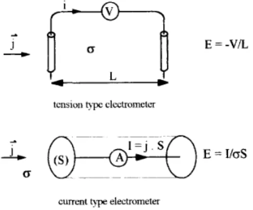
The most usual measurement technique consists in measuring the voltage between two contact points with the sea water (electrodes). This gives the electric field value along
the direction of a line between the two electrodes, after
dividing by the separation distance. Practical implementation of this method has given a large number of different devices, in relation with the origin and the frequency range of the field
to be measured. An extended review of ULF electromagnetic
fields in the sea and associated instrumentation is given in [4].
A new method was recently proposed , based on a current
density measurement [7, 81. Electric field in the sea arise as a
result of electric current flowing through the water, according
to the Ohm's law in conducting media :
-+ -+
J
= o E (13)The volume current density is collected on large plane elec- trodes, between them a lineic current is measured, which
depends on the surface of the electrodes.
In
order to notdisturb the electric field lines, the global impedance of the measurement device must be suited (at ULF frequencies) to the equivalent impedance of the replaced water volume in the measurement direction. So this technique allows to take all
the energy of the signal. Fig. 2 shows the two methods
comparatively.
tension tqpe electrometer
current
+v
electrometerFig. 2. Klectric field measurement methods
We have developed and build a current collection based marine electrometer, with a original current measurement system [9] and special design electrodes. Details of the prototype and different steps of its performing are described
in [4]. The grading of the electrometer was made in laboratory
in a basin with artificial sea water. The test bed is showed on
Fig. 3. The apparatus has a cylindrical grading and disk electrodes. Two subsidiary electrodes (injection electrodes) put on either internal side of the basin allow to impose known electric field.
Because of the impedance suiting criterion, the impedance
of the (reception) electrodes, which is a hnction of the
electrolyte exposed surface and a large number of physical and chemical parameters, has a great importance for the sensitivity of the apparatus and the calculation of its transfer fimction. Furthermore, this impedance induces a voltage
between the microscopic interface electrode - electrolyte, and
so a signal loss for the measure. We have identified from
impedance measurements an equivalent circuit model for the interface electrode-electrolyte (Fig. 4).
For the simulations, we use this model (electrosorption
impedance) with the parameters C, = 0.21F, Cads = 0.83F,
4
= O,971R, and S = 2325cm2.Fig. 4. Circuit model for the electrolyte /electrode intertace
v.
ELECTROMETER MODEL AND FEM RESULTSWe use for the FEM model equations of 111. 2D and 3D
modelisation are performed. Vertical slide of the geometry which is used for the 2D calculations is showed Fig. 5.
i \
Dirichlet Dinchlet
-
Neumann1
Fig. 5. Boundary conditions (FE and BIE Models)
The electrode interfaces in which the potential is rapidly varying are extremely thin (about 10-lOm). Electrode
interfaces are so geometrically described with interfacial
elements (zero thickness) and an equivalent surface conductivity (Eq. 5) corresponding to the impedance model of Fig. 4 and the previously exposed parameters.
The impedance of the internal current detection circuit is
Fig. 3. Marine electrometer in the test basin inductive. For the numerical FEM simulation, this impedance
is modelled by an equivalent volume conductivity:
Satisfactory results are obtained with the first prototype, 0 2 = L/(Z,S)
which has a self noise level about VImIH-'". However, where:
some improvement are even possible. In order to optimise the L = 0,684cm, S = 0.2325cm' , Z2 - = 0,73+i00.0194 1R
The conductivity of the electrolyte is 01 = 4Qm-l,
representative of natural sea water. next prototype without a lot of new experimentations, we
have performed 2D and 3D numerical models of the sensor in the basin.
1687
The casing of the electrometer is described with interfacial
elements and a zero surface conductivity. Boundary condi-
tions are those of Fig. 5.
2D and 3D simulations are perform with those parameters
and frequencies ranging 10” to 10
Hz.
In 3D, only a quarterof the geometry is describe in order to reduce the number of unknowns. The following figures (6 and 7) show respectively
2D and 3D calculated electric potential at frequency of 1
Hz.
E]-/[-
.--.._ ..,-- ...I-
... ...ll:::::::ij
/4/1
... ...[
‘
i
...l
...l
...,_.’
...--
--
,/’ -----
... ... realpart (-IFig. 6. 2D FE Model of the electrometer. Electric potential (f = 1 Hz)
@ c: +I (VI) im. part(-0.09 < @ i 0.09 (VI) 3ectrode
+
1 V lectrolyte7
Electrodes with surf. impedance Elec v Electrode - 1 :Wometer IVFig. 7. 3D FE Model of the electrometer. Electric potential (f = 1Hz)
W.
BOUNDARY INTEGRAL EQUATIONS MODELThe same problem was solved using a BIE model, at the
cost of some slight modifications in a standard software [3].
A. Standard formulation
then (1) becomes a Laplace’s equation:
In the electrolyte region
‘I!
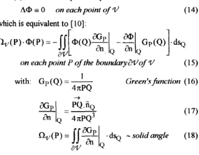
the conductivity is constant,A@ 0 on eachpoint of V (14)
which is equivalent to [lo]: r
on each point P of the boundaryavof V (15)
1 with: Gp(Q) =
-
4nPQ -+-
--a~
Q 4nPQ3 Green’sfinction ( 16)B. Special interface equation
The
B E
(1 5) links together the boundary hnctions @ anda/&
(= [email protected]) and is particularly suitable to take intoaccount the interface equations (3) and (4): when P or Q is on
the interface, we obtain a second link between these functions:
Yo : inner potential of the electrode
The substitution of this equation in (1 5) allows to take into account the electrochemical effect on an electrode with a BIE formulation.
C. Non-confined environment
With this boundary integral method, it is also possible to forecast the response of the electrometer to a given electric
field Eo = -?Do in a boundless electrolyte: the results will
help us t o justify the relative little size of the measurement basin pig. 2).
In this case, @ is not the total electric potential, but
characterises the perturbation of the electric field:
E = - V ( @ o + @ )
(20)@ obeys the Laplace’s equation (and the boundary integral
equation), but the interface equation (1 9) turns :
0.6
0 -5
0.4
D.
Inner i m p e h c e : an equivalent modelThe BIE program we used does not accept circuit
equations. Therefore, the inductive behaviour of the inside of the electrometer was simulated using an equivalent 3D
conduction problem and a fictitious indtictive electrode :
~~ i I Dirichlet ~ @=Vo Dinchlet A
-
’-
NeumanFig 8 BIE model for the inner impedance of the electrometer
E. hxampie of RIliM
3D
resiilt.5.Hectrode a i t h suriace impedance
electrode
f = 1 I I L
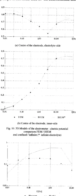
Numerical results are just in correct agreement with
measurements (fig. 11). The difference may be due to the
very simple circuit model used for the electrochemical effect.
.
i
.
0.6
(a) Centre ofthe electrode, electrolyte-side
0.8- 0.7
1
I-
I
b 0.3 t 0.2 I 11
*d 0 . 0 C t----
.---t--- 0.0 1 0.10 1.00 10.00 f[lIz] R1F.M D I E M * 1. E M ~ .~(b) Centre ofthe electrode, inner-side Fig. 10. 3D Models of the electrometer : electric potential
comparison FEM / BLEM
and confined / inlinite (*: infiiite electrolyte)
f = 0.01 Hz
Fig 9 I D BIL Model ofthe cloctrometer Electnc potential at z=O (real part) influence ofthe frequency
I
I VI1 COMPARATIVE RESULTS
4
O.OlL---- - +. ~ -~ c - --c-
0.0 I O x ) LOO 10.00
f [ W
Fig 10 shows the excellent agreement between FE and BIE
models So interfacial elements seem to be validated and could
be used to model other interface phenomena (SVIII) BIE
results for confined and open space are very similar we can expect the electrometer to have the same behaviour in the sea as in the measurement basin
-
Measure ‘ModelI689
WII. EXAIVPLE 2 : THERMOELECTRIC SEEBECK EFFECT
In the first example ($111 to §VII), we have validated that the general interfacial element can be used in order to take
into account direct drops of the unknown (Eq. 4). In this
second example we will compute simultaneous normal and tangential interfacial discontinuities. This kind of boundary conditions is find in the thermoelectric Seebeck effect. A classical analysis of this phenomena [12] leads to:
(1) V(-OV@) = 0
on the domain with boundary conditions:
-
classical continuity, of normal current :(3) (02Zi@2 - ~ l Z i @ l ) . ii = 0 and:
-
thermoelectric effect :A ii - 9 0 2 A ii = (SI - S ~ ) ~ T A ii (22)
where T is the temperature and Si, S2 the thermoelectric powers of each material.
In such a case, the hypothesis H2 cannot be verified. This
problem must be solved by assembling two sets of equations
in the general matrix of the problem : &er a classic Galerkin
moiection :
and :
jjs
Y m i V P k A f i @ k . d S = O ( 2 4 ) kj
where i E interface ofmedia 1
m E interface of media 2
j E volume ofmedia 1
k
E volume ofmedia 201,
P,
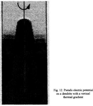
y are the polynomials defined in Fig. 1.The discontinuous pseudo-electric potential has been
computed [SI in the case of an axisymmetric microscopic
dendrite submitted to a vertical thermal gradient (Fig. 12).
CONCLUSION
A general curvilinear interfacial element has been tested in a) continuity of tangential gradient and discontinuity of b) continuity of tangential gradient and discontinuity of c) discontinuity of both tangential and normal gradients at This kind of elements are very powerful in order to solve
order to solve three kinds of discontinuities :
normal gradient in linear interface with a small thickness. normal gradient on surface impedant interface.
the interface.
non-natural boundary conditions in FEM.
Fig. 12. Pseudo electric p on a dendnte with a vn thermal gradient
REFERENCES
utential rtical
[ 11 Ph. Masse, "Modelling of continuous media methodology and computer aided design of finite element programs," IEEE Trans. Mag., vol. 20,
n"5, pp. 1885-1990, 1984.
121 FLlJX-EXPERT user manual. DT2I Corp. , 8 ch. des Preles, ZIRST - 38240 Meylan (France).
[31 L. KrahenbW, A. Nicolas, L. Nicolas, "The CAD package PHUD for the computation of electric or magnetic fields in 3D devices," Compel, vol. 9, [4] V. Poulbot, "Contribution a I'etude des champs electriques tr6s basses fiequences en milieu &anique," Ph. D. Thesis 93-36, Ecole Centrale de Lyon, France, oct. 1993.
[ 5 ] Olivier Laskar, "Phenomenes thermdlectriques et magneto-hydro- d p m i q u e s en solidification des alliages metalliques," Ph. D. Thesis, INP Grenoble, France, jd. 1994.
[ 6 ] J.H. Filloux, "Instrumentation and experimental methods for oceanic studies," J.A. Jacobs (ed.), Geoelectromagnetism I , pp, 143-248, 1989. [7] J. Mosnier, "Dispositif de mesure dun champ electrique dans un fluide
conducteur, et procede utilisant un tel dispositif," French patent, 84
SUPPI. A, pp. 185- 189.
19577 (FR 2 575 296
-
Al), 1986.[SI U. Rakotosoa, "Appareillage de mesure des tres faibles champs electriques en milieu marin. Application a la mise en evidence des signaux electromagnetiques induits dans la mer," Ph. D. Thesis, Paris VI, France, 1989.
[9] R. Blanpain, F. Robach, "ProcBde et dispsitif pour la mesure dun champ Blectrique en milieu conducteur," French patent 9102273, 1991. [IO] L. KrahenbLihl, A. Nicolas, L. Nicolas, "Contraintes electriques dans une
chambre de coupure: une methode danalyse tridimensionnelle," RGE,
oct. 1989: n"9, pp.4449.
[ 1 I] L. Krahenbtkhl, "Surface current and eddy current 3D computation using B E techmques," Digests 3rd in@ IGTE symposium, Graz, Austria, sept. 1988.
[ 121 J.A. Shercliff, "Thermoelectric magnetohydrodynamics," J. Fluid Mech., vol. 91. oart2.00. 231-251. 1979.