On the period length of some special continued fractions

J

OURNAL DE

T

HÉORIE DES

N

OMBRES DE

B

ORDEAUX

R. A. M

OLLIN

H. C. W

ILLIAMS

On the period length of some special continued fractions

Journal de Théorie des Nombres de Bordeaux, tome

4, n

o

_{1 (1992),}

p. 19-42

<http://www.numdam.org/item?id=JTNB_1992__4_1_19_0>

© Université Bordeaux 1, 1992, tous droits réservés.

L’accès aux archives de la revue « Journal de Théorie des Nombres de Bordeaux » (http://jtnb.cedram.org/) implique l’accord avec les condi-tions générales d’utilisation (http://www.numdam.org/conditions). Toute uti-lisation commerciale ou impression systématique est constitutive d’une infraction pénale. Toute copie ou impression de ce fichier doit conte-nir la présente mention de copyright.

Article numérisé dans le cadre du programme Numérisation de documents anciens mathématiques

On

the

_{period length}

of

some

special

continued fractions.

par R. A. MOLLIN AND H. C. WILLIAMS

ABSTRACT. We _investigate and refine a device which we introduced in

[3]

for the _study of continued fractions. This allows us to more _{easily compute}

the _{period lengths} of certain continued fractions and it can be used to

suggest some _aspects of the _cycle structure

_(see

_[1])

within the _period of certain continued fractions related to _underlying real _quadratic fields.

1. Introduction.

Let r and s be

_positive

_integers

with s &#x3E; r ; and define

M(r, s)

to be

the value of n in the continued fraction

expansion

where _qn, &#x3E; 1.

This _may be

_interpreted

as

M(r, s)

=

T(r, s) -

2 where

T(r, s~

is the function of Knuth

_[2,

_p.

_344].

Let

_{gcd(a, q)}

= 1 where a and _q are

_positive

_integers

with

_{a $ 1.}

Set

where 0 Si q and define

where w is the order of a modulo _q, and

L j

denotes the

_greatest

integer

function.

In

_[3]

we

proved

that if

with .

is an

integer

then the continued fraction

_expansion

of

_{(a -}

1-I-

has

_{period length}

1C’

given

by

when

_qan

&#x3E;

a k.

Here x =

n),

d =

gcd(n, k)

and

(Note

that we have made the

assumption

that a, while

arbitrary,

has been

fixed.)

It _seems,

_however,

to be more

_appropriate

to use the function

W(a, q)

defined in

_(1.1).

The reason for this is that we _may

always

assume

that d = 1.

(If d ~

1,

then

replace

a

by

ad, k

by

kld

and n

by

n/d).

Under

the condition that

_{gcd(n, k)}

= 1 we

_get

Bernstein

_[1]

noticed that for certain

_parametric

forms of

_D,

the

con-tinued fraction

_expansion

of

B/D

has a certain

cycle

structure within the

period. Usually

these

_cycles

were not _very

_long,

but in some "remarkable"

cases he found

cycles

of

length

11. In fact it is

possible

to

_develop

certain forms of N for which the

_cycle

structure of the continued fraction

_expansion

of

_{((1’ -1}

+ is

_quite

intricate. A detailed

_description

of this will form the

_subject

of a future _paper. For now we will content ourselves with the

following

example.

Consider the case where _q = a‘‘ - 1 and k = mw. As we shall see in

§2

it is

_possible

in this case to show that

_{W(a, q~}

= 2w - 2.

Therefore,

’

~r = 2n + 3rrlw - 2m when

gcd(n, mw)

= 1 and n &#x3E; mw. If we

_put

we get

7r = (5~ 2013 2)m + 2.

Thus for

a

square-free integer,

we

_get

cycles

in the continued fraction

expansion

of

(u - 1

+ of

_length

5w - 2 when w is fixed. More

_{complicated cycle}

structures can also be

predicted

when we have further results on

W(a, q).

It is _{easy to} show that if m

q/2

then

Hence,

Now,

(in

what follows all summations assume

gcd(m, q)

=

1),

(For

the definition of _T~ see Knuth

[2,

_p.

353]).

By

a result of Porter

[5],

we know that

Also

_§(q)

_q-1

and so we have an _upper bound on the value of

W(a~, q~,

a bound which is

quite good

when _q is a

prime

and a is a

primitive

root of

q. For

example,

2 is a

primitive

root of 37 and

W(2, 37)

= 106

by

direct

calculation,

whereas

The purpose of this paper is to

develop

methods for

improving

the

speed

of

_computing

_{W(a, q)}

_beyond

that of

_simply

_using

_(1.1).

2. Some Alternate

_Expressions

for

_{W(a, q).}

We will show in this section how the work of

_computing

_{W(a, q)}

can be

halved. We first

_require

LEMMA 2.1.

_{Ifxy == 1}

_{(mod q)}

with 0 x, y q then

Proof.

This can be

easily proved by

making

use of results of Perron

[4,

p.

32].

D

We note that since si s,-, m 1

(mod q),

we have :

Hence we can write

when w is odd and

Notice that if _q = a~ 2013

_1,

then for i _W, we have _Si = ai

and q =

a" - 1 =

(aw-’ -

I)st

_{+ ai -} 1

whereas sx

=

a’

=

l(ai - 1)

₊ 1.

Hence,

q)

= 2. It follows from

(1.1)

that

Also, if q =

al’ + 1 thenw =

2J.l

and _Si = ai for i

w/2.

Hence

M(Si,q)

= 1 for i and

_by

_(2.4)

Thus,

if _q = a~’~ ± 1 it is _{easy to} evaluate

W(a, q).

In the next

sev-eral sections we will show how to

_develop

formulas for

_determining

the value of

_{W(a, (a~’~}

::i:

_1)lq)

in terms of

_{W (a, q)}

when all.

_{(mod q).}

We will concentrate on the more difficult

problem

of

finding

the value of

W(a, (a~’~

+

_1)/q)

in terms of the value of

_{W(a, q),}

but will indicate from time to time how the

_{simpler proof}

for the value of

_{W(a, (all. - 1)/q)}

in

terms of

_W(a,

_q)

can be

_developed.

In fact we will show the

following.

Main Results. In sections 4 and 5 we _prove

THEOREM 2.1.

_(see

_5.10).

where A is the least

_{positive integer}

such that

aÀ == -1

_{(mod q),}

a is define end

with

THEOREM 2.2.

_{(see (5.11)).}

If p is

the order of a

_{modulo Q =}

_{(all. -}

_1)lq

&#x3E; q then

In section 6 we conclude with some

Special

Cases. THEOREM 2.3.

_{(see (6.2)).}

THEOREM 2.4.

_{(see (6.3)).}

then

Finally,

THEOREM 2.5.

_{(see (6.4)).}

and

Let j

be an

arbitrary

but fixed

integer

such that

1 ~ j ~ úJ.

Define

y

a~~

(mod q)

and

y*

=

(mod q),

where 0 _q.

Put

_t-2

=

_{t* 2 =}

_{q, t-1}

=

y, t* ~ _

7*

and define

ti, ti

by

Also,

put

for i= -1,0,1,2, ...

and

where

_Q

is as in Theorem

2.2,

Q* _

(a~’, + 1)~q &#x3E;

3 and S %

a~

_{(mod Q),}

S* - aj

_{(mod Q*).}

If

_{M(y, q)}

is even, then m =

M(y, q),

tm,

= 0 and

_tm-l

= 1. If

M(y, q)

is odd then m =

M(y, q)

_{+ 1.} We

replace

the value of

by

that of

pm-i - 1 and

put

pm =

1,

= 0,

= 1 and = 1. We deal with

the continued fraction

_expansion

of

_q/y*

in the same _way.

The purpose of this section is to relate the value of M to that of m and

the value of M* to that of m* . We divide the

_problem

into 2 cases.

Define r-2 = q and

We have that _{r -1,}

_{r* ~ ,}

_ro,

_{r* 0}

are

integers.

Thus for i &#x3E; -2 we have that _r; and

_r7

are

integers.

Proof. The result

_certainly

holds for i =

-2, -1,

0. Also the result holds if i is even. Now since rz is an

_integer

we

_get

Thus,

if i is odd and r;

0,

then we can

only

have

r*

= 0. But

r*

= 0

only

A7 .

Since

we

_get

Thus,

gcd

0

_(mod

whence = 1. It follows that i - 1 = m* - 1 or i - 1 = m*-2. Since m* is even and i is odd

we get

i = m* -

1,

which is

impossible

since i m* - 1.

LEMMA 3.2. ~f -2 i m* - 3 then

_r7

&#x3E;

_ri+l.

Proof. The result is

_certainly

true for 1

_{= -2, -1.}

Now if i &#x3E;

_0,

thus if i is _even, we

_get

rg

&#x3E; If i is

_odd,

i m* - 3 and then

_{ri =}

_{~+~ .}

° For

and

Thus

where _{81, S2} are

integers,

and

If

_{I -}

_{then 81 - s2}

0. Now

_A~

+

_{A~_~}

~1~. = ~ ;

thus,

if 81 -

~2 7~

0,

then 81 - s2 -1 and which is

_impossible.

Hence si = _S2

r* 1.

Also,

hence,

and,

Since

_Ai+l

I = q we =

1,

and I =

By

the

same

reasoning

as that used in Lemma 3.1 we can now _prove Lemma 3.2.

D

We use the notation to denote the fractional

part

of _any real x;

i.e.,

~x} =

x -

Lxj.

We are now able to _prove

THEOREM 3.3.

_{If q ~}

2 and aJ

_Q*

then M* = m*

+ 4

when aJ &#x3E;

_2q

and &#x3E;

_1/2,

M* = m* - 2 when aJ

q/2

and _&#x3E;

1~2 ;

otherwise,

M* = m* + 2 when a-7 _&#x3E;

2q/3

and M* = m* when a3

2q/3.

Proof. For convenience we will use the

symbol k

to

represent

m*. We

Case A.

aj

q.

From

_(3.1)

we have

Ak-l 1*

- 1

_{(mod q);}

_hence,

~~~

_{(mod q)}

and _{q -}

_aj,

since 0

_Åk-l

_{Ak -}

q. It follows that

Ak_2

-q -- and

pj

=

lq/(q -

Thus

pj

= 1 if and

only

if

aj

q/2.

Also,

if

_1,

then

_{tk_2 = 1}

and

_{Ak_2 =}

aj.

By

definition

_{of rk-l}

we

_get

_rk-l

=

0,

hence k &#x3E; 1. Also

_{tk-3 = JJk-l}

+1

and

_Ak-3

= =

q - aj

t~_;~ .

From this we can deduce that

rk_2 - 1

and

_{’~l-3 ~}

_{rk-2 - Pk-2.}

If

_{~k_Z &#x3E; 1}

then

_{rk_~ &#x3E;}

&#x3E;

_rk-l

= 0.

By

Lemmas 3.1 and 3.2 we see that

M(9~0")

= k - 1: J

Since k is even we have M* = k = m*.

If

_JJk-2

=

1, then rk-3 = rk_2

= 1.

and M* = m* - 2. Now

Also 1 if and

_only

if

_{A~_2 /A~ _;~}

2,

which holds if and

_only

if

or

if li*

&#x3E;

1,

we

_get

and

Since

_{tk-2 =1=}

1,

we cannot have i

thus,

Since &#x3E; we see that

r~ = ~ - 1 = 1

if and

_only

if 2

_{q/(q -}

_aj)

3 ;

i.e.,

q/2

2q/3.

Also 2 if and

only

if

a3

&#x3E;

_2q/3.

Case &#x3E; q.

By

(3.2)

with i = k - 3 we must have &#x3E; rk_2. Also &#x3E;

_rk-~

A~

= _q. Since

1,

this can occur if and

_only

_iftk-2

=

J-lk

= 1. In this

case we

_get

_1,

and =

rk-l + rg =

+ l)rk-l

-~-1. Hence

_{M(,5’*, ~*)}

= k + 1 and = m* _{+ 2. Now} = 1 if and

only

if 2.

_Also,

since

2013~

_{(mod q)}

and q, we

_get

0

_Ak-l

=

_{tq - aj}

_q, where t = ~’ Since

Ag

= _q we see that

tk-l

= 1 if and

only

if

1/2.

We have seen that if &#x3E; 1 then &#x3E;

_{rk .}

Also

If

_l~l

= 2 then

M(5’~~)

= k + 2 and M* = m* + 2. If

ri

_&#x3E; 2 then

r~

=

1(r~ - 1) -f- l,

M(,5’*, Q*) _ ~

₊ 3 and M* = m* + 4.

Also, r:r"

= 2 if and

_only

if

aj

+

2q.

Since

-aj

_{(mod q),}

this can hold if

and

_only

if q

aJ

2q.

Collecting

all of the above we

_get

the Theorem.

D THEOREM 3.4.

If aj

_Q

then M = m + 2 &#x3E; q and M = m when

aJ

q.

Proof. Use similar

_reasoning

on the r; sequence to

get

results similar to

Lemmas 3.1 - 3.2. The result then follows.

D Case 2.

_Q

_(Q*

_aj)

Here we define _{r -2} = _q and

where h _{= /~ 2013}

_j.

In _{this case /)} =

~y~

=

ah

_q.

By

using

methods similar to those used above we can _prove.

LEMMA 3.5. If -2 i m" - 3 then

_r7

&#x3E; 0. LEMMA 3.6.

If -2 i m* - 5

then

_r7

&#x3E;

_r*i

THEOREM 3.7. If

ai

&#x3E;

_Q

then M* = m* - 4 when

Q*

a h/2

and &#x3E;

_1/2,

M* = m* + 2 when

Q*

_&#x3E;

2a h

and

&#x3E; 1/2 ;

otherwise,

M* = m* - 2 when

Q

2a~/3

and M* = m* when

Q

_&#x3E;

2ahy3.

THEOREM 3.8. Ifa~ &#x3E;

_Q

then M = m-2 when

ah &#x3E;

Q

and M = m when

Q.

In the next sections we refine some of these results.

4. Some Refinements.

We will need to

_put

Theorems 3.3 and 3.7 into forms in which we can use them to relate

_W(a,Q*)

to

_W(a,q).

We do that in this section. LEMMA 4.1.

_{If j}

&#x3E; 0 and h

_{= p - j}

then

_Lah’/Q*J.

Proof. +

₁₎

= ₊

a h)

which is

_impossible.

It follows that =

0 LEMMA 4.2. &#x3E;

_1/2

if and

_only

if &#x3E;

_1/2

Proof. Let _q =

a-7m,

_{+ ri} for 0 _ri

al,

and

ah~

=

Q*M2

_{+ r2} for

By

Lemma 4.1 we have that = _mi =

rn2 =

Lah./Q*j.

_Also,

since

LEMMA 4.3. then

_Q*

_a~/2

if and

_only

_q/2.

Proof.

_{If Q*}

ah

then

_(a11’+I)/q

_{a h /2,}

_q &#x3E; and q &#x3E;

If _q &#x3E;

2ai,

we must have

ah &#x3E;

2. For if

ah

=

1,

then p = j

and

Q* =

(a’ +

1)/q.

Since

_Q*

&#x3E; 1 we would have _q

ai

which is not

possible.

Also

if q

&#x3E;

2a~ -~-1 = 2(a~ -~ 1/2) &#x3E; 2(a~’-h --~ a-h) &#x3E;

2a -h (a/"

-E-1).

It follows that

_Q*

_{ah /2.}

_{(here gcd(Q*, a)}

= 1 and h &#x3E;

1).

’

0’

°

LEMMA 4.4. then

_Q*

_{2ah /3}

if and

_only

if aj

_2q/3.

Proof. If

_Q*

_{2ah /3}

then

a3’

+

a-h

_2q/3

and

a3*

_2q/3.

If

aj

_2q/3

then

a 1,,-h

_2q/3

and 3a" =

2qah - k for k

_&#x3E; 0. Since k - 0

_(mod

_{ah )}

we have k &#x3E;

a h

and it follows that a’"

2qah /3 - ah/3.

If

ah /3

&#x3E;

1,

then

Q* =

(all.

+

_1)lq

2a~/3.

If

_{ah /3}

_1,

then h =

1,

a =

2, 3.

If

ah

= 3 then 3’"

_{2q -}

1 and

_{q &#x3E;}

_(31"

+

_1)/2

which means that

Q*

_2,

an

impossibility.

By

similar

_reasoning

it is

_possible

to exclude the case where

ah

= 2. 0

By

using

the same kind of

_reasoning

as that used above we can also

prove.

LEMMA 4.5. then

_Q*

&#x3E;

2ah

if and

_only

if a-7 &#x3E;

_2q.

LEMMA 4.6. then = and _&#x3E;

1/2

If and

_only

_{if la3lql}

&#x3E;

_1/2.

With these results we can now

give

a different version of Theorem 3. ~ .

THEOREM 4.7. &#x3E;

_Q

then M* = m* - 4 when a~

q/2

and

iqlail

&#x3E;

_1/2,

M* = m* -f- 2 when _&#x3E;

2q

and

la-7

/q}

_&#x3E;

1/2 ;

_,.

otherwise,

M* = m* - 2 when a3

_2q/3

and M* = m* &#x3E;

_2q/3.

We define the

_symbols

and

We can now combine the results of Theorems 3.3 and

_4.7;

(recalling

the

definition

_{of Xj}

_given

in theorem

_2.1).

THEOREM 4.8.

_{and j}

_p, then

_M~

=

mj +

2x~ - 2qj

+

2~j

when

_Q*

&#x3E; q.

Proof. We note that if _e~ = 0

then qj

= 0. First assume _p.

Case 1. _ei = 0.

In this case

Q*

_{&#x3E; q}

implies

that aJ &#x3E; q, hence

Case 2. _ej = 1. In this case aj

_Q*.

Case

_2a.

= 0. Here aJ &#x3E;

_2q/3

and M* = m* + 2 +

_2Xj

= m* + Case

_{2b. i7j}

= 1. Here a3

2q/3

and M* = m* ₊

2X3

= m* ₊

2Xj -

₊

2e.

..

We note that

_M*

= 2 and

m*

= 0. Also in this case

and we

get ai

&#x3E;

_2q.

Hence

_0,

_qj = 0. Furthermore

5. The formulas.

We are now in a

_position

to derive the formulas

_relating

_W(a,Q)

and

W(a, Q*)

to

_{W(a, q).}

If v is the order of a modulo

Q*

then

LEMMA 5.1. 3

_{and p}

is the least

_{positive integer}

such that a’--1

-0

_(mod

_Q*)

then v =

Proof.

_Certainly

_{2p % 0}

_{(mod v).}

If v is odd

_{then p}

= 0

_{(mod v).}

In this

case -1 -

(a~’)"~~’

= a" == 1

(mod Q*)

and

Q*

divides 2 which contradicts that

_{Q* &#x3E;}

3.

_{Thus, v}

is even and

(= v/2)

divides _p. Put A = Since

let

_{Q* =}

where a" - 1

(mod

and a’~ - -1

(mod Q2 ).

Hence,

= 1

_(mod

and al’ = 1

_{(mod Qi)}

whence

_Q,

is even. If

Q1

= 1

then a’~ - -1

_{(mod Q*).}

_By

definition

_{of p}

we must but since

p = 0

_{(mod ~)}

we _p, and v =

2p.

If

_{Qi =2}

and

_QZ

is

_odd,

then since aK == -1

_{(mod 2)}

we

_get

that

a’ - -1

_{(mod Q*);}

_{whence, v}

=

_{2~. Suppose Q1 =}

2 and

C~2

=

2’-’

Q’

with s - 1 &#x3E; 1. If

_Q*

= 2..

Q’

does _not divide _{aK + 1 then}

2..-1

_properly

divides a’’~ + 1 and a" = -1 +

2’-’ t

for odd t.

Now,

-1 - a’l. =

aÀIâ.

_

(-1 )~‘’ -f- 2!-~ at

(mod 2.").

If A is even then 2.. divides 2 which is

impossible.

If A is odd then 2 q divides

2.,,-1

At ;

i.e. At is even which is also

impossible.

Thus K = _p.

D Note that we _may also assume that

if Q* _

(a~’ -+-1)/q,

then _p is the least

positive integer

such that al’ - -1

_(mod

_Q*).

_For,

if this is not the _case, then

_{suppose A}

is the least such

_{integer. By}

Lemma 5.1 we have that 2A

divides

₂

or A divides _J1.. Since

a

- -1

_{(mod Q*)}

we

_get

_q

= q’

a -- I for some

_{integer q’.}

It follows that we can write

* _

(a

-+-1)/q’

for q’

_q.

Thus

_by

_replacing

the value

_{of p by}

that of A and the value

_{of q by}

that of

q’,

we have the form of

_Q*

which is desired.

In view of the above remarks we can now rewrite 5.1 as

(by 2.4).

Now

Since a’l. m -1

_{(mod q),}

there is a least

positive A

such that

a~

m -1

(mod q)

and w = 2A.

Also Jl ==

0

(mod A), K

= is odd and

7 =

Thus

By

(2.4)

we have

Since

_ml

= 0 we

_get

By

Theorem 4.8 and

_(5.2)

we

_get

We now need to evaluate each of these sums. We note that

Since we

_get,

whence,

It follows that

Thus, by

(5.3)

we

_get

Recall that a is defined

_by

a° _q

a’+’.

Thus we find that

Thus

Also

Thus

where

However,

since

_3a°/4

a° _q we have = and

It remains to evaluate

_r

_Xi. We first prove

2=1

LEMMA 5.2.

_{If j}

₂

A + 2 then _Xx+j = 1.

Proof. We first note that

_{since j}

_~&#x3E;

A + 2 we have

Thus

and

Now

Thus,

the result follows.

Since

and K is odd we

_get

by

lemma then

q =

2B +I (here

_a =

2).

In this _case

get 22À+1 ==

2

_{(mod q);}

thus

_1/2

when A &#x3E; 1 _{and X2p+1} = o.

Thus,

3 and

_{a ~}

2 then when

aÀ+1

_2q

we

_get

X2p+1 = 0. Since 0 lnce 0 2 we

_get

a’

we

get

Xp+1 +

= 1 -

L2q/aÀ+1J

unless _q = 3and a = 2 in which case = 1. With the

_exception

of _{this case we}

get

Given the definition of

_{S(a, q)}

in Theorem 2.1 we see that it

_depends

for its value

_only

on the values of a and _q. Now

{r/s} &#x3E; 1/2

_implies

_that

L2r/sj -

2Lr/sj

=

_1,

and

1/2

implies

L2r/sj -

2Lr/sj

=

0 ;

thus,

we can write

The

_[2/aj

term here occurs because =

1/2

when _al = 2. Also

If we

_put

together

the formulas

_(5.3)-(5.7)

and

_(5.9)

we

_get

(here

2,

3 and

_Q*

&#x3E;

_q).

This is Theorem 2.1.

By

using

the results of section 3 we can also derive

_by

much

_simpler

under the

_assumption

_{that p}

is the order of a modulo

Q,

(an

assumption

which can be made without loss of

generality),

and the

assumption

that

q

Q.

This is Theorem 2.2.

6.

_Special

Cases.

In this section we will

develop

formulas for

W(a, q)

for certain

special

values of _q. We first note that when _q =

aa

₊

1,

then we can

easily

evaluate

S(a, q).

We have

that ai

_q/2

_{for j}

=

1, 2 ~ ~ ~ ,

a - 1. For such values of

j

we

_get

- .

and

unless

ai =

2.

Since

_q/2

aÀ

_2q,

we

_get

Now, when q

=

a~

_{+ 1 and}

Q*

=

(all’

₊

1)/(a-B

₊

1)

is an

integer

larger

than

2,

then _p m 0

_{(mod A)}

and we have

LEMMA 6.1.

_IfQ*

is

_{as given}

_above,

_{A 0}

_1,

and

_{a 0}

_2,

then the least value

v such that a’ m 20131

_{(mod Q*)}

is _~.

Proof. Let K = Since 2v is the order of a modulo

Q*

and m 1

(mod

Q*)

we have 2v

dividing

2AK or AK m 0

_{(mod v).}

Put v = for

&#x3E; 1. Since = -1

_(mod

20132013-)

_wegetthata+1

_{(a + I) (a + 1)}

t &#x3E;

1. Since a’ == 1

(mod

a -t- 1

we

_get

that

a

₊ 1

(a"

+

₁₎

(a

+

₁₎

Since

Q*

&#x3E; 1 we must have &#x3E; 1 and since K is odd we must have K &#x3E; 3.

Also, v &#x3E; 1,

and À 1. If then

AK - v - A &#x3E;

1 and

Hence,

or

It follows that

_{(t - l~(~c - 1~ 1 +t/a.}

Since K &#x3E;

_3,

we have that

2(t - 1~

1 +

_t/A

or 2t -

t/A

3.

If t = 3,

this can

only

occur for A - 1. But from

(6.1)

we

_get

whence

which means that a =

2 ;

this value is excluded

by hypothesis..If t

= 2 then A is even and A &#x3E; 2. If A &#x3E;

_2,

then 2t -

_t/A

&#x3E; 2t -

_t/2

&#x3E;

_3t/2

&#x3E;

_3,

which is

_impossible.

If t = 2 and A =

_2,

then

by

(6.1)

and we

_get

a contradiction. Hence we must have t = 1 and v = AK = _~.

0

By

using

similar

_techniques

it is _{easy to prove}

LEMMA 6.2. and

_Q

=

(all. -

1)

is an

_integer

_greater

than I then the order of a

_{modulo Q}

is _p.

From Lemma 6.2 and

_(5.11)

_{with q}

= a~’ - 1 we

_get

cx = cv - 1 and

which is Theorem 2.3.

we get

2q

&#x3E;

a’ for

1 I A and

_{S(a, q) = 0.}

Furthermore,

c~ ==

A,

= 1 and

W(a,q)

= 4A - 2

_by

(2.6).

Hence

by

Lemma 6.1 and

(5.10)

we

_get

where e is as in Theorem 2.4 which is now

_proved.

It should be noted that we have

only proved

(6.3)

when

aa

+ 1

_~

3.

However,

it can be

easily

shown that in this case

This holds because

_M*(2~,(2~’

+

_1)/3)

= 4 for 3

k p -

2 and

1)/3)

= 2.

Thus (6.3)

holds for

a~ - 1 = 3.

We have also excluded the case

where q

=

2,

but it is also _easy to show that

Thus

_by

_(2.4)

we

_get

which is Theorem 2.5.

Undoubtedly

many more results

_concerning

this remarkable function

W (a, q)

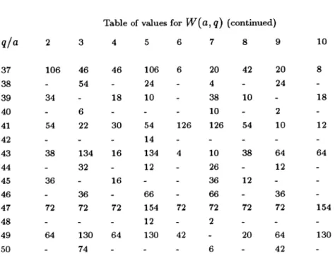
remain to be discovered. We conclude this _paper with a short

Table of Values for Parameters :

Table of values for

_q)

_(continued)

Acknowledgements :

The author’s research is

_supported

_by

NSERC Canada

_grants

No. A8484 and No. A7649

_{respectively.}

REFERENCES

[1]

L. _BERNSTEIN, Fundamental units and _cycles, J. Number _Theory 8

_{(1976), 446-491.}

[2]

D.E. KNUTH, The Art of _{Computer Programing} II : Seminumerical _Algorithms,

Addison-Wesley, 1981.

[3]

R.A. MOLLIN and H.C. _WILLIAMS, Consecutive _{powers in} continued _fractions,

(to

appear : Acta

Arithmetica).

[4]

O. PERRON, Die Lehre von den Kettenbrüchen, Chelsea, New-York

(undated).

[5]

J.W. _PORTER, On a theorem of Heilbronn, Mathematika 22

(1975),

20-28.

Department of Mathematics and Statistics

University of _Calgary

Calgary, Alberta T2N 1N4 Canada

e-mail: _{ramollin@ac+ucalgary.ca.}

Computer Science _Department

University of Manitoba

Winnipeg, Manitoba R3T 2N2

Canada