HAL Id: hal-03191101
https://hal.inria.fr/hal-03191101
Submitted on 11 May 2021
HAL is a multi-disciplinary open access
archive for the deposit and dissemination of
sci-entific research documents, whether they are
pub-lished or not. The documents may come from
teaching and research institutions in France or
abroad, or from public or private research centers.
L’archive ouverte pluridisciplinaire HAL, est
destinée au dépôt et à la diffusion de documents
scientifiques de niveau recherche, publiés ou non,
émanant des établissements d’enseignement et de
recherche français ou étrangers, des laboratoires
publics ou privés.
Distributed under a Creative Commons Attribution - NonCommercial| 4.0 International
Lionel Mattéo, Isabelle Manighetti, Yuliya Tarabalka, Jean-michel Gaucel,
Martijn van den Ende, Antoine Mercier, Onur Tasar, Nicolas Girard,
Frédérique Leclerc, Tiziano Giampetro, et al.
To cite this version:
Lionel Mattéo, Isabelle Manighetti, Yuliya Tarabalka, Jean-michel Gaucel, Martijn van den Ende,
et al..
Automatic fault mapping in remote optical images and topographic data with deep
learning.
Journal of Geophysical Research : Solid Earth, American Geophysical Union, 2021,
1. Introduction
Fractures and faults are widespread in the Earth's crust, and associated with telluric hazards, including tectonic earthquakes, induced seismicity, landslides, rock reservoir fracturing and seepage, among others (e.g., Scholz, 2019). While fractures are generally small-scale, shallow, planar cracks in rocks (Barton & Zoback, 1992; Bonnet et al., 2001; Segall & Pollard, 1983), faults span a broad range of length scales (10−6– 103 km) and surface-to-depth widths (1–102 km), and have a complex 3D architecture (e.g., Tapponnier & Molnar, 1977; Wesnousky, 1988). At all scales faults form dense networks (“fault zones”) including a master fault and myriads of secondary fractures and faults that intensely dissect the host rock embedding the mas-ter fault, sometimes up to large distances away from the masmas-ter fault (Figure 1) (Chester & Logan, 1986; Granier, 1985; Manighetti, King, & Sammis, 2004; Mitchell & Faulkner, 2009; Perrin, Manighetti, & Gaude-mer, 2016; Smith et al., 2011). This intense secondary fracturing/faulting off the master fault is referred to as “damage” and has been extensively studied in the last decades (Cowie & Scholz, 1992; Faulkner et al., 2011; Manighetti, King, & Sammis, 2004; Perrin, Manighetti, Ampuero, et al., 2016; Savage & Brodsky, 2011; Zang et al., 2000) because it provides clues to understand fault mechanics. In particular, intense fracturing makes damaged rocks more compliant than the intact host material, which in turn impacts the master fault be-havior (Bürgmann et al., 1994; Perrin, Manighetti, Ampuero, et al., 2016; Schlagenhauf et al., 2008). This issue is of particular importance when the master fault is seismogenic, that is, has the capacity to produce earthquakes. The architecture and the mechanical properties of the fault zone have indeed a strong impact on the earthquake behavior on the master fault: they partly control the rupture initiation and arrest and thus the rupture extent, but also the amplitude of the ground displacements and accelerations and thus the
Abstract
Faults form dense, complex multi-scale networks generally featuring a master fault and myriads of smaller-scale faults and fractures off its trace, often referred to as damage. Quantification of the architecture of these complex networks is critical to understanding fault and earthquake mechanics. Commonly, faults are mapped manually in the field or from optical images and topographic data through the recognition of the specific curvilinear traces they form at the ground surface. However, manual mapping is time-consuming, which limits our capacity to produce complete representations and measurements of the fault networks. To overcome this problem, we have adopted a machine learning approach, namely a U-Net Convolutional Neural Network (CNN), to automate the identification and mapping of fractures and faults in optical images and topographic data. Intentionally, we trained the CNN with a moderate amount of manually created fracture and fault maps of low resolution and basic quality, extracted from one type of optical images (standard camera photographs of the ground surface). Based on a number of performance tests, we select the best performing model, MRef, and demonstrate its capacity to predict fractures and faults accurately in image data of various types and resolutions (ground photographs, drone and satellite images and topographic data). MRef exhibits good generalization capacities, making it a viable tool for fast and accurate mapping of fracture and fault networks in image and topographic data. The MRef model can thus be used to analyze fault organization, geometry, and statistics at various scales, key information to understand fault and earthquake mechanics.© 2021. The Authors.
This is an open access article under the terms of the Creative Commons Attribution-NonCommercial-NoDerivs
License, which permits use and distribution in any medium, provided the original work is properly cited, the use is non-commercial and no modifications or adaptations are made.
Lionel Mattéo1 , Isabelle Manighetti1 , Yuliya Tarabalka2, Jean-Michel Gaucel3,
Martijn van den Ende1 , Antoine Mercier1 , Onur Tasar4, Nicolas Girard4,
Frédérique Leclerc1 , Tiziano Giampetro1, Stéphane Dominguez5 , and
Jacques Malavieille5
1Université Côte d'Azur, Observatoire de la Côte d'Azur, IRD, CNRS, Géoazur, Sophia Antipolis, France, 2LuxCarta,
Sophia Antipolis, France, 3Thales Alenia Space, Cannes, France, 4Université Côte d'Azur, Inria, Sophia Antipolis,
France, 5Université de Montpellier, Géosciences Montpellier, Montpellier, France Key Points:
• We adapt a U-Net Convolutional Neural Network to automate fracture and fault mapping in optical images and topographic data
• We provide a trained model MRef
able to identify and map fractures and faults accurately in image data of various types and resolutions • We use MRef to analyze fault
organization, patterns, densities, orientations and lengths in six fault sites in western USA
Supporting Information:
Supporting Information may be found in the online version of this article.
Correspondence to:
L. Mattéo,
Citation:
Mattéo, L., Manighetti, I., Tarabalka, Y., Gaucel, J.-M., van den Ende, M., Mercier, A., et al. (2021). Automatic fault mapping in remote optical images and topographic data with deep learning. Journal of
Geophysical Research: Solid Earth, 126, e2020JB021269. https://doi. org/10.1029/2020JB021269
Received 28 OCT 2020 Accepted 25 MAR 2021
Special Section:
Machine Learning for Solid Earth Observation, Modeling, and Understanding
earthquake magnitude and harmful potential (Hutchison et al., 2020; Manighetti, Campillo, Bouley, & Cot-ton, 2007; Oral et al., 2020; Radiguet et al., 2009; Stirling et al., 1996; Thakur et al., 2020; Wesnousky, 2006). Given the prominent role of damage zones in fault and earthquake mechanics, accurate quantification of the 3D architecture of faults is of primary importance. At depth, this determination is still challenging as most geophysical imaging techniques rely on a number of assumptions and lack the resolution to dis-criminate the multiple closely spaced fractures and faults off the master fault “plane” (Yang, 2015; Zigone et al., 2019), while borehole provide valuable yet local observations (e.g., Bradbury et al., 2007; Morrow et al., 2015).
Alternatively, most faults intersect the ground surface, where they form clear traces generally with a foot-print in the topography (Figure 1). These traces offer a great opportunity to observe most of the fault zone architecture at the ground surface. Therefore, most fault observations over the last century have been made at the ground surface, and rendered into 2D maps reporting the surface fault traces. Historically, these maps
Figure 1. Optical images of fault traces at ground surface, at different scales. Fault traces appear as dark lineaments in images, forming dense networks. At all
scales, more pronounced, master fault traces (red arrows, not exhaustive) are “surrounded” (on one or both sides) by dense networks of closely space secondary faults and fractures of various lengths, generally oblique to and splaying off the master fault trace. (a and b) Pléiades satellite images of Waterpocket region, USA (ID in data statement). Two fault families are observed on (a), trending ∼NNE-SSW and ∼WNW-ESE. In both images, some of the faults have a vertical component of slip and thus form topographic escarpments that are seen through the shadows they form. (c and d) hand-held camera ground images in Granite Dells, USA; in (c) secondary faults splay from the underlined master trace, forming a fan at its tip; in (d), the underlined master fault trace is flanked on either sides by a narrow zone of intense fracturing, generally referred to as inner damage. Note the color change across the densely fractured inner damage zone.
were produced directly in the field from visual observations of the surface fault traces and the measurement of their characteristics (strike, dip, slip mode, and net displacements), and were reported as trace maps with specific attributes (e.g., Watterson et al., 1996). Over the last few decades however, the rapidly expanding volume of satellite and other remote sensing data has greatly assisted the fault trace mapping. Under ap-propriate conditions (e.g., no cloud overcast for optical images), surface fault traces (and fracture traces, depending on data resolution) are clearly seen in remote images and topographic data, and can thus be analyzed remotely. Optical images are most commonly used for fault trace analysis, as the faults appear as clear and sharp sub-linear or curvilinear “lines” of pronounced color gradients (e.g., Chorowicz et al., 1994; Manighetti, Tapponnier, Gillot, et al., 1998; Tapponnier & Molnar, 1977).
Accurately mapping fault and fracture traces requires a specific expertize as these traces have complex, curvilinear shapes and assemble, connect or intersect in an even more complex manner, yet partly deter-ministic (Figure 1). Because this complexity arises from the master fault growth and mechanics, it is of prime importance that it is properly recovered in the fault trace maps. Fault mapping is thus an expert task that requires a rich experience in fault observation and a fair understanding of fault mechanics. Would oversimplified or overlooked mapping be done, the signature of the mechanical processes would be lost and the faults left misunderstood. However, even when the fault mapping is done by an expert, various sources of uncertainties affect the mapping (e.g., Bond, 2015; Godefroy et al., 2020, and see below). The expert map-ping is commonly done manually: the expert recognizes the fracture and fault traces visually in the remote images (and possibly other data), and reproduces these traces as hand-drawn lines in a Geographic Infor-mation System (GIS) environment. These environments allow fault attributes such as trace hierarchical importance, thickness, interruptions, connections, and slip mode to be labeled in various ways (various line thicknesses, colors, symbols, etc.) (e.g., Flodin & Aydin, 2004; Manighetti, Tapponnier, Gillot, et al., 1998). Some of the uncertainties on fault traces can also be informed.
Manual mapping of fault and fracture traces by an expert is arguably the most accurate processing tech-nique. However, it is extremely time consuming, while the expertize might not be always available, which prohibits the analysis of large areas at high resolution, and dramatically limits the amount of available accurate fault maps. Edge detection algorithms have been proposed (e.g., Canny, 1986; Grompone von Gioi et al., 2012; Sobel, 2014) and used to automate fault mapping in image data, as these algorithms can rapidly extract all the objects expressed as a strong gradient in the images. However, these edge detectors generally suffer from poor accuracy and do not always discriminate fractures and faults from other linear features, especially in textured images (Drouyer, 2020). Another semi-automated approach named Ant-tracking (Monsen et al., 2011; Yan et al., 2013) has been developed to detect linear discontinuities in optical images but it needs heavy pre-processing of the images (for instance, to remove vegetation) and a priori constraints on the faults that are searched for (orientations, curvature, etc.). Other sophisticated approaches, based on stochastic modeling and ranking learning system, have demonstrated high efficiency to detect curvilinear structures in images (Jeong, Tarabalka, Nisse, & Zerubia, 2016; Jeong, Tarabalka, & Zerubia, 2015), but these approaches require to set many a priori parameters to define the structures that are searched for, and were never applied to faults.
Therefore, an automatic solution for rapid and accurate fracture and fault mapping in optical images would be greatly beneficial to better characterize the structural, geometric, and hence mechanical properties of fault zones. Here, we propose to address this challenge using deep machine learning, and more specifically, a Convolutional Neural Network (CNN) model (LeCun, Haffner, et al., 1999). Machine learning comprises a plethora of numerical methods that can learn from available data and make predictions in unseen data (process called generalization, e.g., Abu-Mostafa et al., 2012; Goodfellow, Bengio, et al., 2016). Machine learning is not a new domain of research, with the first landmark works having emerged in the 50–60's (see Figure 1 in Dramsch (2020) and references therein). However, its demands for large quantities of data and computational resources required by the learning process have only been met over the last two decades or so (e.g., Bishop, 1995; Carbonell et al., 1983; Devilee et al., 1999; Ermini et al., 2005; Goodfellow, Bengio, et al., 2016; LeCun, Bengio, & Hinton, 2015; MacKay, 2003; Meier et al., 2007; Mjolsness & DeCoste, 2001; Van der Baan & Jutten, 2000). This has spawned numerous applications in computer vision, natural lan-guage processing, and behavioral analysis (Sturman et al., 2020; Voulodimos et al., 2018; Young et al., 2018). Among the various algorithms, CNNs have shown great potential to tackle the complex task of image data
analysis (medical, satellite, etc.) and the capacity to rapidly process vast volumes of data (e.g., Krizhevsky et al., 2012; Russakovsky et al., 2015; Simonyan & Zisserman, 2014). In most computer vision tasks, CNNs indeed achieve state-of-the-art performance.
Currently, there is a rapidly expanding number of scientific works developing and or applying CNNs and oth-er machine learning techniques to assist researchoth-ers in detecting, modeling, or predicting specific features in a broad range of domains, including medical sciences (e.g., Ronneberger et al., 2015; Shen et al., 2017), remote sensing (e.g., Lary et al., 2016; Maggiori et al., 2017; Tasar, Tarabalka, & Alliez, 2019), chemistry (e.g., Schütt et al., 2017), climate sciences (e.g., Rolnick et al., 2019), engineering (e.g., Drouyer, 2020), and geosciences (e.g., Bergen et al., 2019). In the domain of geosciences, machine learning methods have es-pecially flourished in earthquake seismology (e.g., Hulbert, Rouet-Leduc, Jolivet, & Johnson, 2020; Kong et al., 2019; Mousavi & Beroza, 2020; Perol et al., 2018; Ross, Meier, & Hauksson, 2018; Ross, Meier, Hauks-son, & Heaton, 2018; Rouet-Leduc, Hulbert, & Johnson, 2019; Rouet-Leduc, Hulbert, McBrearty, & John-son, 2020; Zhu & Beroza, 2019), and seismic and geophysical imaging of the Earth's interior with a major focus on sub-surface image interpretation for resource exploration (e.g., Babakhin et al., 2019; Dramsch & Lüthje, 2018; Gramstad & Nickel, 2018; Haber et al., 2019; Meier et al., 2007; Waldeland et al., 2018; Wu & Zhang, 2018). A few other works have been conducted in oceanography (Bézenac et al., 2019), geode-sy (Rouet-Leduc, Hulbert, McBrearty, & Johnson, 2020), volcanology (Ren, Peltier, et al., 2020), and rock physics (Hulbert, Rouet-Leduc, Johnson, et al., 2019; Ren, Dorostkar, et al., 2019; Rouet-Leduc, Hulbert, Lubbers, et al., 2017; Srinivasan et al., 2018; You et al., 2020). However, few works have been conducted so far to address fault issues with machine learning, and all of them have targeted seismic images, that is, transformed vertical images of the Earth interior where actual faults cannot be observed directly (Araya-Po-lo et al., 2017; Guitton, 2018; Tingdahl & De Rooij, 2005; Wu and Fomel, 2018; Zhang et al., 2019). As far as we know, there has been no study addressing the identification and mapping of tectonic fractures and faults directly observable in optical images of the Earth ground surface.
In the present study, we leverage recent deep learning developments for this task. We have adapted a CNN with U-Net architecture (Ronneberger et al., 2015) from Tasar, Tarabalka, and Alliez (2019), which was orig-inally dedicated to identify buildings, roads, and vegetation in optical satellite images, to the challenge of fault and fracture detection. We develop a reference model, MRef, that we train with a small amount of image data and basic manual mapping, so as to simulate the common situation where only rough manual fault maps and few images are available. We apply MRef to different types of images (hand-held camera, drone, satellite) at distant sites, and demonstrate that it predicts the location of faults and fractures in images better than existing edge detection algorithms, and at a high level of accuracy similar to, and possibly greater than, expert fault mapping capacities. Using a standard vectorization algorithm, we analyze the MRef predictions to measure the geometrical properties of the fault zones. We provide the trained reference model MRef as a new powerful tool to assist Earth scientists to rapidly identify and map complex fault zones in ground imag-es and quantify some of their geometrical characteristics.
2. Image, Topographic, and Fault Data
2.1. Fault Sites
We analyze faults in two distant sites differing in context, geology, fault slip modes and fault patterns, as well as in ground morphology and texture (Figure 2). In both sites, faults are inactive (i.e., currently not accommodating deformation) and were exhumed from several km depth (de Joussineau et al., 2007; DeWitt et al., 2008).
The first site, “Granite Dells,” is a large granite rock outcrop (∼15 km2) with sparse vegetation, in central Arizona, USA (Haddad et al., 2012) (Figures 2a and 2b). The granite, of Proterozoic age, is dissected by a dense network of fractures and faults spanning a broad range of lengths from millimeters to kilometers (Figures 3a–3g). While the fractures are short open cracks with no relative motion, the faults are longer features with clear evidence of lateral slip (en echelon segmentation, pull-apart connections, slickensides). They have no or little vertical slip preserved and therefore they hardly imprint the topography (i.e., no or small escarpment), but where they have sustained differential erosion (Figures 2b and 3a–3g). Overall, frac-tures and faults organize in two families, trending about NE-SW and NW-SE and cross-cutting each other,
yet with no clear systematic chronological relationship. The fracture and fault density is extremely high throughout the site, making their manual mapping difficult and time consuming.
A second site, “Valley of Fire,” is a large outcrop (∼30 km2) of the Jurassic Aztec Sandstones formation, in southern Nevada, USA (de Joussineau & Aydin, 2007; Myers & Aydin, 2004) (Figure 2c). The site is desertic and thus has no vegetation. It is densely dissected by faults of meters to kilometers of length, showing clear evidence of both lateral (left- and right-lateral) and vertical (normal) thus oblique slip (Figures 2c, 2d, 3h,
Figure 2. (a and b) Granite Dells, Arizona and (c and d) Valley of Fire, Nevada sites. (a and c) show Pléiades satellite images of the sites (ID in data statement),
with location of the sub-sites analyzed in present study. (b and d) show field views of some of the faults and fractures (photographs courtesy of I. Manighetti). Note the vertical component of slip on some of them, forming topographic escarpments. In Granite Dells (b), most fracture and fault traces are surrounded by an alteration front (darker color).
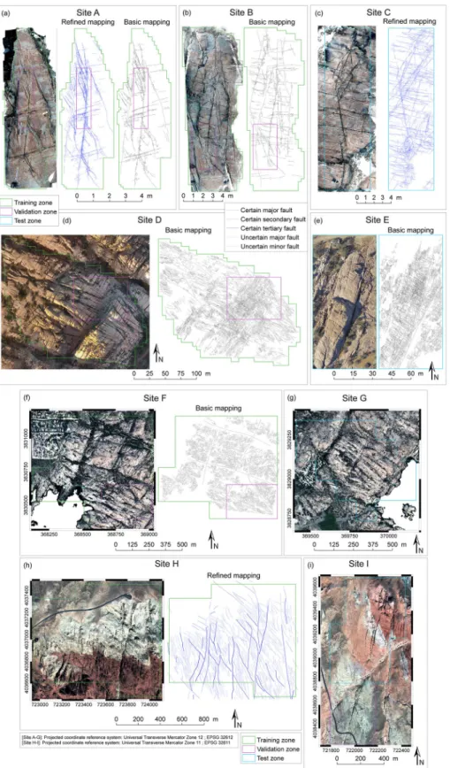
Figure 3. Sites, images, and ground truth fault maps used in present study. (a–g) from Granite Dells site, (h–i) from Valley of Fire site. (a–c): hand-held camera
ground images, (d and e): drone images, (f–i): Pléiades satellite images (ID in data statement). Training, validation and test zones are indicated in green, purple and blue, respectively. Sites C and G are only used as test zones. Basic (black) and refined (blue) mapping were done manually (not shown on Site I for figure clarity). Fault hierarchy is indicated only in refined maps in (a, c, and h) through different line thicknesses, but is most visible when zooming the figures out. Dotted lines are for uncertain fractures and faults. Note, in most sites, the very high density of fractures and faults, the existence of different fault families with various orientations, and the presence of non-tectonic features. Also note that, in all sites, the manual mapping is incomplete (as exhaustive manual mapping is practically unachievable).
and 3i) (de Joussineau & Aydin, 2007). Most faults have thus formed topographic escarpments from meters to tens of meters high. Faults organize in two principal families trending about N-S and NW-SE (Ahmadov et al., 2007; Myers & Aydin, 2004).
2.2. Optical Image and Topographic Data
To document fractures and faults over a broad range of lengths from mms to kms, we have acquired differ-ent types of optical images on six subregions within the two sites (Figure 2), amounting to a total of ∼4,600 individual images over the two sites. We have then used Structure from Motion (SfM) photogrammetric technique (e.g., Bemis et al., 2014; Bonilla-Sierra et al., 2015; Harwin & Lucieer, 2012; Turner et al., 2012) to calculate, from the individual images, both the topography of each subregion (Digital Surface Model or DSM) and its ortho-image (rectified mosaic-like global image). The six subregions being almost free of veg-etation, the DSM are equivalent to the DTM (Digital Terrain Model) most commonly used. The resolutions of the DSM and the ortho-images are here the same.
We have acquired four types of images (Figures 2 and 3, and Table 1):
(a) In three subregions of the Granite Dells area later referred to as Sites A, B, and C (Figures 2a and 3a–3c), we have acquired a total of 165 RGB photos “on the ground” with a standard optical camera (Panasonic Lumix GX80) elevated by 3 m above the ground. Sites A, B, and C are about 3, 6, and 7 m wide and 10, 15, and 20 m long, respectively. The ortho-images and DSMs (calculated with Agisoft Metashape software, AgiSoft Metashape Professional (Version 1.4.4, 2018; http://agisoft.com) of Sites A, B, and C have an ultra-high resolution of 0.5, 1.2, and 1.3 mm, respectively. They thus allow recovery of frac-tures and faults down to a few millimeters in length, while the extent of the surveys limits the longest recovered faults to 10–15 m (Table 1). As we could not acquire GPS ground control points in the sites, the ortho-images and DSMs are not geo-referenced. However, to ease their description, we will refer to as “North,” “South,” “West,” and “East” for the Top, Bottom, Left and Right sides of the images, respectively
(b) In two other subregions of the Granite Dells site referred to as Sites D and E (Figures 2a, 3d, and 3e), we have acquired ∼40 RGB photos from an optical camera onboard a drone (DJI Phantom 4) flying less than 100 m above ground level. Sites D and E are about 230 × 150 m2 and 50 × 100 m2, respectively. Their ortho-images and DSMs, here georeferenced, have a high resolution of 2.4 and 1 cm, respectively, allowing recovery of fractures and faults down to a few centimeters of length, while the longest recov-ered faults are a few 10–100 m long (Table 1)
Site Number of images in training data set (green) Number of images in validation data set (pink) Number of images in test data set
(blue) Number of images in total data set Total area of analyzed zone (m2) Spatial resolution of image & DSM (m) Fault length range (m) Approximate vertical resolution of DSM (m) Type of mapping A 1,365 203 – 1,568 25.7 0.5 × 10⁻³ 0.001–10 0.005 Refined (HR) & basic
B 809 120 – 929 87.7 1.2 × 10⁻³ 0.001–10 0.01 Basic C – – 912 912 101.0 1.3 × 10⁻³ 0.001–10 0.01 Refined (VHR) D 678 154 – 832 31.4 × 10³ 24 × 10−3 0.01–100 0.5 Basic E – – 325 325 6.9 × 10³ 10 × 10−3 0.01–100 0.5 Basic F 30 6 – 36 590 × 103 0.5 10–700 1 Basic G – – 19 19 310 × 103 0.5 10–400 1 Basic H 63 – – 63 1,032 × 103 0.5 10–1,000 1 Refined (HR) I – 12 29 41 670 × 103 0.5 10–1,000 1 Basic
Note. Each image refers here to a 256 × 256 pixels tile.
Abbreviation: HR, high resolution; VHR, very high resolution.
Table 1
(c) Over the Granite Dells site, we have also acquired three Pléiades satellite optical images with different view angles (ID in data citations), which we use to analyze two subregions referred to as Sites F and G (Figures 2a, 3f, and 3g). Each Pléiades image is delivered as two files, one panchromatic image with one band at a resolution of 50 cm, and one multispectral image with four bands at a resolution of 2 m. Using the panchromatic tri-stereo images, we calculated a DSM of the site at 50 cm resolution (Micmac soft-ware, free open-source solution for photogrammetry, see Rupnik, Daakir, & Deseilligny, 2017; Rupnik, Deseillignya, et al., 2016). Then, using the multispectral Pléiades image with the view angle closest to the Nadir, we derived a color ortho-image of the site. To calculate the color ortho-image at 50 cm reso-lution, we used pansharpening techniques from GDAL/OGR (2018) to fuse the highest resolution pan-chromatic image with the lower resolution multispectral image. The F and G sites are ∼900 × 790 m2 and 760 × 640 m2, respectively, and therefore the longest recovered faults are 400–700 m long. Although the resolution of the images is high, the smallest faults that are well resolved are ∼10 m long
(d) In the Valley of Fire site, we have acquired three Pléiades satellite optical images (ID in data citations) with different view angles to analyze two subregions referred to as Sites H and I (Figures 2c, 3h, and 3i). As above, we calculated a DSM and an ortho-image of Sites H and I at 50 cm resolution. The H and I sites are ∼1.1 × 1 km2 and 1.4 × 0.6 km2, respectively, so that the longest recovered faults are about 1 km long. Although the resolution of the images is high, the smallest faults that are well resolved are ∼10 m long
2.3. Fault Ground Truth Derived From Manual Mapping
Manual fault mapping of parts of the sites is used as ground truth to train the CNN models. Fractures and faults were hand-mapped in the images and topographic data following common procedures in active tectonics (e.g., Manighetti, Tapponnier, Courtillot, et al., 1997; Manighetti, Tapponnier, Gillot, et al., 1998; Tapponnier & Molnar, 1977; Watterson et al., 1996). Mapping was done with Erdas Ermapper ( www.geosys-tems.fr) or QGIS (QGIS Development Team, 2020). Faults are represented by curvilinear lines of different thicknesses made to inform on the fault hierarchy (major vs. minor faults, see below). It has to be noted that this information on fault hierarchy is provided to assist the tectonic analysis, but is not used in the deep learning training (it is a further scope). Fault maps are eventually stored as shapefiles, that is, vector files containing geographic information.
To explore which level of expertize in fault mapping is needed to properly train the Deep Learning models, we produced three qualities of mapping (Table 1):
• Sites A, B, D, E, and F were mapped by a student with limited expertize in fault mapping (Figure 3). This produces a comparatively low resolution ground truth, where fault traces are simplified while many mi-nor fractures and faults are missing and the fault hierarchy is not indicated. These mappings are referred to as “basic” in the following
• Site A and H were mapped by an expert geologist, yet at a moderate resolution (Figures 3a and 3h). This means that while most faults are mapped accurately and their hierarchy informed, some details in their trace are simplified while the smallest fractures and faults are not mapped. The expert mapping is referred to as “refined” in the following
• Site C was mapped by an expert geologist, at the highest possible resolution (Figure 3c). This means that all fractures and faults visible up to the highest resolution of the data were mapped as accurately as pos-sible, with their hierarchy informed. The C fault map is thus the most exhaustive ground truth
In the refined fault maps, faults traces are discriminated into 3 levels of hierarchy during the mapping, using lines of different thickness (Figures 3a–3h): from thicker to thinner lines, (1) the major faults which have the most pronounced and generally the longest traces, and hence likely accommodate the greatest displacements, (2) the secondary faults and fractures, which have less pronounced but still clear traces and are generally of shorter length, and (3) the tertiary faults and fractures which have subtle traces, commonly looking like very thin cracks in the rock. It has to be noted that, because displacement typically varies along a fault (e.g., Manighetti, King, Gaudemer, et al., 2001), the thickness of the line made to represent a fault trace can vary along its length. Again, the information on fault hierarchy is provided to assist the tectonic analysis, but is not used in the following deep learning training.
Regardless of the degree of expertize to produce the manual fault mapping, the drawn fault traces have four uncertainties: (1) a fault trace generally looks as a dark, thick lineament of several pixels width in optical images. This width results from different causes, including the real thickness of the fault trace (from mm to m depending on fault size, e.g., Sibson, 2003), the existence of intense fracturing juxtaposed to the fault trace (see Figure 1d), the apparent widening of the fault trace due to a vertical component (see shadows in Figures 1a–1c), and the weathering of the fault trace at the ground surface. Generally, the exact position of the fault (i.e., the exact intersection “line” between the fault plane and the ground surface) cannot be as-sessed accurately within this several-pixels wide trace, even by the best expert; (2) Even in cases where the fault trace is clear, its drawing by the user cannot have a pixel-wise resolution: for a matter of time, mapping is commonly done at a lower resolution than the image pixel. The mapping thus conveys uncertainties, especially where the fault trace is tenuous, and when the mapping is done at low resolution (as in the basic mapping here); (3) some fault traces are uncertain; while they look like fault traces, they might represent other features, like alteration zones or erosion patterns. Where such an ambiguity arises, the uncertain fault traces are represented by dotted lines; (4) depending on the scale and resolution at which the data is analyzed, some faults may not have been mapped while they do exist in the outcrop; exhaustive manual mapping is practically unachievable. Therefore, the fault ground truth is inevitably incomplete and holding uncertainties.
The fault shapefiles are converted into raster maps where each pixel is assigned a probability to be a fault. If actual fault traces would be one-pixel lines, the fault pixels would be assigned a probability of 1 (i.e., being a fracture or a fault), while all other pixels in the image would be assigned a probability of 0 (i.e., not being a fracture or a fault). To account for the uncertainties described above as items 1 and 2, we applied to the fault map raster a 2D Gaussian filter (Deng & Cahill, 1993) with a standard deviation of 0.8 pixels. The 2D Gaussian filter acts as a point-spread function: it assigns a probability of 1 (i.e., being a fracture or a fault) to the pixels along the drawn fault lines, and a probability decreasing in a Gaussian manner from 1 to 0 to the 3 pixels-wide zone either side (probabilities normalized after Gaussian spreading). Furthermore, along uncertain faults (dotted lines, and uncertainty described above as item 3), the largest probability is set to 0.5. Together these make the ground truth fault lines having a 7 pixels width and a heterogeneous probability distribution ranging from 0 (i.e., 100% certainty that it is not a fracture or a fault) to 1 (i.e., 100% certainty that it is a fracture or a fault).
In summary, the data used as input in the CNN algorithm described below include aligned optical images, DSMs and ground truth fault probability maps, organized in two files: (1) the optical images (3 bands) and the DSM (1 band) are concatenated into a 3D array (4 bands) of pixel values, and (2) the ground truth fault probability map is provided as a 2D array of probability pixel values.
3. Deep Learning Methodology
We use a CNN of U-Net architecture that we have adapted from Tasar, Tarabalka, and Alliez (2019). The algorithm is written in Python, and employs the TensorFlow library (https://www.tensorflow.org/about/ bib; Abadi et al., 2015).
3.1. Principles of Deep Learning and Convolutional Neural Networks
Here we present a mostly qualitative description of the Deep Learning methods employed in this study, aiming to provide a general overview of our approach. For a more quantitative exposition of the methodol-ogies, we refer to Text S1.
In many situations, relatively simple relationships can be established between two quantities. While these relationships are not necessarily linear or physically interpretable, they can be easily visualized and identi-fied owing to their low-dimensional character (i.e., they can be captured in a two-dimensional graph). On the other hand, some relationships are more abstract and much harder to characterize; one prime example is that of individual pixels in an image and their relationship to the contents of the image (e.g., a human face, an animal, a tectonic fault, etc.). While a single pixel does not uniquely define the contents of the image, it is the arrangement and ordering of pixels of particular color and intensity that are
interpreta-ble by an observer. This makes the mapping from the input (image pixels) to the output (image contents) high-dimensional. The human brain excels at creating such abstract, high-dimensional relationships, but reproducing this flexibility with computational systems (e.g., in computer vision tasks) has traditionally been challenging.
As a subclass of Machine Learning algorithms, Deep Learning draws inspiration from the human brain, allowing Artificial Neural Networks (ANN) to “learn” from the input data through incremental updates of computational units that are colloquially referred to as “neurons” (see LeCun, Bengio, & Hinton, 2015 for a review). The input data can be already interpreted (these interpreted data are called “ground truth,” and the learning is said “supervised”), or not (unsupervised learning), and there exist combinations. ANNs attempt to find an optimal relationship between the input y and output
ˆy defined by a set of parameters
, often called “weights” and “biases.” During “training” of the model, the parameters are incrementally adjusted by the network to optimize a pre-defined cost (or loss) function. The relationship between y and ˆy may not be obvious to describe in terms of interpretable criteria, but it may be empirically approximated by a large number of non-linear functions and their parameters. While the analogy between biological and artificial neural networks is mostly symbolic, ANNs nonetheless achieve state-of-the-art performance in abstract tasks such as computer vision and text interpretation.Practically speaking, ANNs are constructed in a hierarchical fashion in which the parameters are grouped in layers. A given input vector y is passed onto the first layer, defined by a set of parametrized functions, to produce an intermediate output y1. This intermediate output is passed onto a subsequent layer to produce the next output y2, and this procedure is repeated several times until the terminal layer in the ANN produces the final model output ˆy. While the functions inside each layer are simple (see Text S1) and typically charac-terized by only two parameters (a “weight” and a “bias,” the former being a matrix and the latter a vector), the non-linear combination of a multitude of such functions permits an abstract and extremely high-di-mensional transformation from the input to the output. In a supervised setting (as adopted in this study), the output of the model ˆy is compared with a pre-defined ground truth y, and during the training phase the parameters within each layer are incrementally modified to minimize the difference between the model output and the ground truth. The details of the types and number of functions used in each layer, as well as the number of layers and the cost function that measures the difference between the model output and the ground truth, all fall under the header of the model “architecture.” This architecture is chosen by the user depending on the task to be performed, the type and volume of input data, and the available computational capacities. The architecture parameters (number of filters, blocks, layers, loss function, etc.) are set manu-ally and called “hyper-parameters,” by opposition to the model “parameters” (such as filter weights) which are calculated by the network.
One of the most common architectures employed in numerous scientific domains is the CNN (Fukush-ima, 1975; LeCun, Bengio, & Hinton, 2015) and its variations. By design, CNNs leverage the notion that spatial and temporal data (e.g., time series, images, and video or sound clips) are mostly locally correlated: 2 pixels that are close together in an image are more likely to be part of the same object than 2 pixels that are far away. Each layer in a CNN consists of kernels (also called “filters,” represented by small matrices) that process a small part of the input data at a given time, and that are reused at every location within the data set (Text S1). Intuitively, this reusing of the kernels can be envisioned as sliding each of them through an image or a time series so as to examine a specific feature in the image or data (e.g., an edge with a particular orientation, another type of motif, a combination of motifs, etc.), and then constructing an output holding information on this specific feature. This “scanning” of the input data by the kernels occurs through the multiplication of the input image pixel values with the weights of the filter matrix and can be represented mathematically as a convolution operation (hence the term “Convolutional Neural Network”) (Figure A1 in Text S1).
For the task of pixel-wise classification (i.e., assigning a label to each pixel in the image), a CNN takes an image (either a single-channel greyscale or multi-channel color image as is the case here) as an input to the first layer, which produces a layer output that is proportional in size to the input image, possibly with a different number of channels. The layer output is then passed onto subsequent layers as described above. A given channel of the intermediate output is often referred to as “feature map” as it is constructed by a convolutional kernel that is said to represent a “feature.” In spite of this terminology, a single kernel does
not necessarily represent a well-defined object in the input image, and the interpretation of CNNs (and ANNs in general) has thus proven to be a challenging topic of ongoing research. A typical CNN contains many layers with kernels that hierarchically interact to collectively extract the relevant objects in an image. In general, the more complex the image and the searched objects, the “deeper” the CNN needs to be (i.e., greater number of layers and kernels). A common interpretation is that early layers extract simple patterns such as edges, corners, etc., while deeper layers make combinations of these primitives to extract more complex patterns and shapes, with the final layers extracting complete objects (e.g., Lee et al., 2009). For deep CNNs, the number of filters that “scan” the input image is very high, often counting up to thousands to millions. It is important to keep in mind that these filters are not pre-defined by the user, but learned by the network (Text S1).
3.2. Architecture of the CNN Model Used in Present Study
We have adapted the CNN model developed by Tasar, Tarabalka, and Alliez (2019) to originally detect and map buildings, high vegetation, roads, railways and water in optical images (Figure 4). This CNN is a variant of a U-Net architecture (Ronneberger et al., 2015), which, as any U-Net, includes two sub-networks, called encoder and decoder, with skip connections between the encoder and decoder units.
The main role of the encoder is to extract the objects of concern (called “context”) that contribute to final predictions; conversely, the role of the decoder is to synthesize these features into a prediction and locate them accurately. The encoder is a “contracting path” because it down-samples the data and coarse-grains them through “pooling layers,” generally added after each or a short series of convolutional layers (Text S1). The pooling operation consists in a sliding window that scans the output of the previous layer, looking for the average (“mean pooling”) or the maximum (“max pooling”) value at each position of the scan (Boureau et al., 2010). The pooling operations thus reduce the size of the feature maps, and allow the next filters to have a larger field of view of the data, and thus the capacity to identify larger motifs. Here we use max pooling layers.
Because the encoder down-samples the data, the searched features can be accurately detected but their localization is not recovered accurately. Therefore, a decoder sub-network is added to perform the comple-mentary operation: it up-scales the data (it is thus an “expanding path”) and enables the localization of the identified features. To facilitate the encoding-decoding process, the model is here designed to be symmetric, with the output of each block in the encoder being concatenated to the input of its symmetrical counterpart in the decoder. These concatenations, or “skip connections,” regularize the training process by smoothing the high-dimensional loss landscape defined by the loss function (see Section 3.3), leading to faster con-vergence to the global minimum (Li et al., 2018). Each block in the decoder performs the same number of convolution operations as its counterpart in the encoder, but which are followed by an up-scaling operation
Figure 4. Architecture of U-Net CNN used in present study. See text for detailed description. DSM, Digital Surface
Model; ReLU, Rectified Linear Unit.
128 256 512 512 512 512 512 512 512 512 512 512 512512512512 2 1 5 2 1 5 2 1 5 512 6 5 2 6 5 2 2 1 5 256 6 5 2 128 8 2 1 128 128 128 256 256 256 128 128 4 6 64
Input tile (image + DSM) Feature map
Output probability map Skip connection
Convolutional layer + ReLU Block 1
Block 2 Block 3
Block 4 Block 5 Block 5’ Block 4’
Block 3’
Block 2’ Block 1’ Max-pooling
Convolutional layer De-convolutional layer + ReLU
Encoder Decoder
64 Latent
in the form of a strided deconvolution layer. More details can be found in Tasar, Tarabalka, and Alliez (2019) and in Text S1.
Here, both the encoder and the decoder have 13 convolutional layers, and one central layer that forms the “latent space” (see below) (Figure 4). The 13 layers of the encoder are distributed over five blocks. Each of the first two blocks contains two convolutional layers while each of the three other blocks are composed of three convolutional layers. The convolutional layers of the first block each comprises 64 3 × 3 convolutional filters. The number of filters increases by a factor of 2 in the next blocks until reaching 512 filters in blocks 4 and 5. To ensure that the center of each 3 × 3 filter corresponds to the first pixel of the input image, a padding of 1 is applied to the image (i.e., a border of 1 pixel of value zero is added to the input image, to match the outermost line of the matrix) (Figure A1 in Text S1). Each filter then slides by 1 pixel-step over the image (“stride” of 1 pixel). Each convolutional layer is followed with a standard rectified linear unit (ReLU) function, aimed to introduce non-linearity in the model, and the resulting feature maps are down-sampled with a 2 × 2 max-pooling layer that reduces the resolution of the feature maps by a factor 2. During the encoding process, the characteristics of the input data are summarized in a compact set of numbers stored in the central latent space. The decoder is symmetric to the encoder and thus also consists of five blocks. The first four blocks are composed of one deconvolutional layer and three convolutional layers, and the last block includes one deconvolutional layer and one convolutional layer. The final layer in the network is a convolution layer with a single filter, followed by a sigmoid activation function to ensure that the output falls between 0 and 1 (so that the output can be interpreted as a confidence score). The weights and biases of the filters are updated at each iteration of the training stage using an Adam optimizer (Kingma & Ba, 2014) with a fast learning rate of 0.0001. The weights are randomly initialized following Glorot and Bengio (2010). No regularization (dropout, batch normalization, L2-regularization, etc.) was performed.
3.3. Training Procedure
The available data are 3 bands-optical images, topographic data and manual fault maps. For each site, we have merged the image and topographic data so as to obtain a four bands data set (red, green, blue, and to-pography). In the following, we refer to this data as “image” even though it includes topographic data. The total available data is split into a training set, a validation set, and a test set. To prevent overfitting, we split the data by assigning dedicated regions of the mapped areas (see Figure 3). Limited by the GPU on-board memory availability, to train the CNN models we have split each data set into small tiles called “patches” of 256 × 256 pixels and we have grouped in a batch (a set of patches), 12 of such patches picked randomly in the training data.
Owing to the relatively small volume of ground truth data available for training, overfitting of the model might occur during the training. Over-fitting is when the model learns so much from a specific data set that it becomes unable to predict anything else than this data set. To prevent overfitting, we artificially aug-mented the data set by applying geometrical and numerical transformations, including random horizontal rotations (here we used rotations by 90°, 180°, and 270°), flip transformations, color adjustments (with changes in contrast and gamma correction), and the addition of Gaussian noise (Buslaev et al., 2020). The degree of overfitting is monitored during training by evaluating the model performance on an independent validation data set, which is not used to constrain the model parameters directly. Training of the model is arrested when the model performance on the validation set systematically decreases, while simultaneously the model performance increases on the training set (a primary indicator of overfitting) – see Figure S2 for the stopping criterion for MRef.
To evaluate the performance of the model during the training, we use the cross entropy loss function which is more sensitive to confident false classifications than a mean-squared error function (Nielsen, 2015). As a first step here, we adopt a binary classification approach, assigning to each pixel a class “fault” or “not a fault” (i.e., fault hierarchy is not taken into account). To account for the uneven distribution of fractures and faults in the image data, we use the proportion of “not-a-fault” pixels as a weight parameter (; calculated
according to the training and validation sites that are used to train and validate the current model) in the cross entropy calculation. The weighted binary cross entropy loss () is the average calculated from each pixel (n) of the ground truth (y) and the prediction (ˆy) expressed as follows (Equation 1; Sudre et al., 2017):
1 ˆ 1 n log 1 log 1 ˆ i i i i i L y y y y n (1)3.4. Estimating the Performance of the Models
The performance of the models is first estimated in a qualitative manner, on the one hand through the visual inspections of the results (i.e., fracture and fault probability maps), and on the other hand through the comparison of the results with those obtained with the most common available algorithms, such as edge detectors. We specifically use an edge detection algorithm that computes color gradients in the images (from Canny, 1986; later referred to as “Canny edge filter”), and another one which selects linear gradients (from Grompone von Gioi et al., 2012; later referred to as “GVG detector”). We also compare the results with those obtained with CNN models having different hyper-parameters or a different architecture.
We then quantify the performance of the models. Among the various CNN models that we calculate, the performance is first measured on the validation data sets, in order to select the most appropriate architec-ture and hyper-parameters for the CNN model. We refer to this most appropriate model as the “reference” model, MRef. We then demonstrate the robustness of MRef through its application to independent test data sets (different sites and images, Table 1) that were never seen during the training or the validation.
Because neither the ground truth fault maps nor the model predictions are binary 0 and 1 values, we use a performance metric that handles continuous probabilities. We have chosen the Tversky index (TI, Equa-tion 2, Tversky, 1977), a variant of the most common Intersection over Union (IoU) metrics. The latter measures the ratio between the summed number of pixels (expressed as an area) whose prediction is con-sistent with the ground truth, and the total area encompassing both the ground truth and the predictions, yet only applies to binary data. The Tversky index is more flexible as it can be applied to continuous proba-bilities, while it also takes into account (1) the small proportion of pixels being a fracture or a fault in an oth-erwise dominantly un-fractured area, and (2) the incomplete ground truth, in which some fractures or faults might have not been mapped while they actually exist and are well predicted by the model. The TI metric (
0 TI 1) is calculated per pixel, then summed over the pixel population n, as follows (Equation 2):
1 1 * T ˆ ˆ I 1 ˆ 1 1 ˆ n i i i n i i i i i i i y y y y y y y y (2) The coefficient γ denotes the proportion of “certain” fractures and faults in y; it is thus the number of pixels of probability greater than 0 normalized to the total number of pixels in the image. In the sites studied hereγ is less than 1% on average. Therefore, yyˆ evaluates the pixels detected as fractures or faults in both the
ground truth and the prediction,
1y y
ˆ measures the fractures and faults that are predicted by the model but do not exist in the ground truth, and y
1yˆ
measures the fractures and faults that exist in the ground truth but are not predicted by the model. The two latter terms are weighted by to account for sparsity of fractures and faults in the site. A TI value of 1 indicates a perfect prediction, with a value of 0 indicating the converse. Note that, in this TI calculation, only certain fractures and faults are considered in the ground truth.To compare our results with those of prior works, we also use common metrics such as the receiving oper-ating characteristic (ROC) curve, which compares the “False positive rate” (predicted fault/fracture location not present in the ground truth) to the “True positive rate” (predicted fault/fracture location present in the ground truth) at increasing probability thresholds. With this metric good model performance is character-ized by a low False positive rate and a high True positive rate.
To further measure the accuracy of the reference model (MRef), we qualitatively compare the density, azi-muth and length distributions of the ground truth and the predicted fractures and faults in the validation zone. Finally, we test the robustness of MRef through its application to unseen data sets of different types (different types of images, such as drone and Pléiades, Table 1).
4. Defining a “Reference Model” M
RefIn this section and the following, we discuss the qualitative results in both the entire validation or test zone, and in a smaller “reference” area chosen for its tectonic complexity.
4.1. Selecting the Most Appropriate CNN Architecture
To explore which architecture and model hyper-parameters are the most appropriate for fracture and fault detection in the given image data, we set-up seven U-Net models with different numbers of filters, blocks, layers, and loss functions. While we could not explore the entire range of possibilities, we examined the CNN architectures most commonly used in prior works (see Ide & Kurita, 2017; Ronneberger et al., 2015; Tasar, Tarabalka, & Alliez, 2019).
We designed seven models differing from our reference architecture MRef described in Section 3:
– One model (referred to as MA1) with an architecture as described in Section 3, but using a Mean Squared Error (MSE) loss function
– One model (referred to as MA2) with an architecture as described in Section 3, yet lacking the last block 5 of the encoder and the corresponding block 5' in the decoder
– Five models (referred to as MA3 to MA7) with an architecture as described in Section 3, yet having 2, 4, 8, 16, and 32 filters in the first layer, respectively, instead of 64 in the reference architecture MRef
All these models were trained on the same data. To have a large and homogeneous training data set, we used the basic mapping ground truth on Sites A and B (green zones in Figures 3a and 3b, including a total of 2,174 tiles of 256 × 256 pixels). We then estimated the TI scores of the models in the validation zones (in pink in Figures 3a and 3b, including a total of 323 tiles of 256 × 256 pixels). Using basic fault maps as train-ing data simulates the common situation where only rough manual fault maps are available.
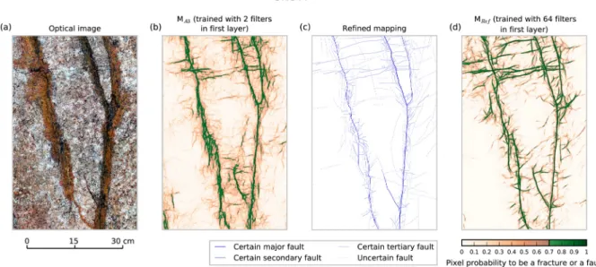
Because a refined ground truth exists in Site A but not in Site B, two TI values are calculated: (1) a TIR calcu-lated only in Site A with reference to the refined ground truth, and (2) a TIB calcucalcu-lated in both Sites A and B with reference to the basic ground truth. In the latter case, we average the two TI values. Figure S3 shows the TI values for the seven models MA1 to MA7 and the reference architecture MRef used with the same data sets. First, for all models but MA1, the TIR calculated with reference to the refined mapping is systematically slightly lower than the TIB calculated with reference to the basic mapping. The difference is likely due to the training done with a ground truth not containing as many details as the refined fault map, leading to a mod-el unable to make predictions at sufficient detail. The difference is small however, and both TI values peak at 0.67 ± 0.01 for the best MRef model. Looking at the models individually, MA1 delivers the lowest TI (0.35), almost twice lower than the TI of the reference model, demonstrating the importance of the loss function. Reducing the number of blocks in the architecture of the CNN from 5 (MRef) to 4 (MA2) does not have a strong impact on the performance of the model (TIB and TIR of 0.63 and 0.59, respectively). In contrast, the number of filters in the first layer of the model has a significant impact on the results. While 16 filters (MA6) might be sufficient to get a reasonable result (TI of 0.62–0.64), a minimum of 32 filters (MA7) is suggested to obtain near-optimal performance. It is interesting to note that, based on the visual inspection of the results, the simplest model MA3 with only two filters in the first block predicts the major and secondary faults fairly well (Figure S4), as well as some of the more minor features (Figure 5b). The model also recognizes that the ruler in the left bottom corner of Figure S4 does not correspond to a fracture, in spite of its straight features and sharp contrast with its surroundings. Furthermore, most predictions at moderate probabilities (0.4–0.6) underline real cracks in the rock (compare Figures 5a and 5b). Some of these were labeled as “uncertain” faults in the ground truth (Figure S4c), but most were not mapped. Therefore, although having only a small number of parameters, the MA3 2-filter model already provides a realistic view of the cracks and faults distribution in the site. The more expressive (i.e., larger) MA7 model provides a prediction almost as good as MRef (Figure S3), yet with slightly larger uncertainties on fault locations (“thicker” probability “lines”), and more apparent “noise” in the form of short fractures with low probabilities (Figure S5). However, when looking at these short fractures in more details (Figure S5b), we can see that most of these do coincide with real cracks in the rock.
Therefore, while the larger model MRef is better performing from a metrics point of view and in its capacity to locate the major faults with high fidelity (narrow probability lines), the smaller models and especially the smallest 2-filter model provide realistic fracture and fault predictions down to the smallest scales, with an apparent greater capacity to predict the smallest cracks than has MRef. This likely results from the models having been trained with basic mapping ignoring small fractures. Because the adopted loss function pe-nalizes any differences between the model output and the ground truth (regardless of whether or not the ground truth is accurate), any model trained on the basic mapping will be biased toward ignoring small-scale details that are absent in the basic ground truth. However, because these small-small-scale details are subtle, a more expressive model is more likely to learn this implicit bias than do the less expressive, smaller models.
4.2. Sensitivity of Model Performance to Training Data Size
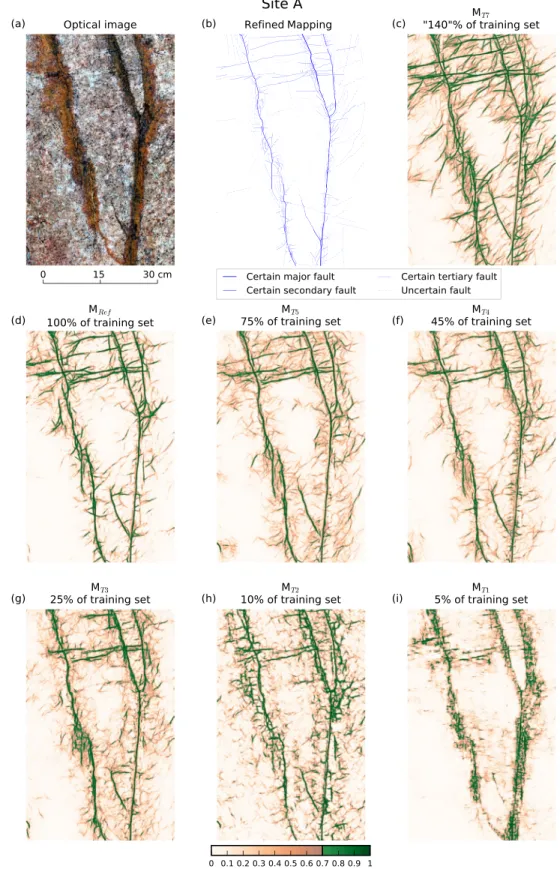
To assess the prediction capacities of the reference architecture, we explore the impact of the size of the training set on the performance of the models. To generate consistent comparisons, we use the same data sets as in the prior section. Within the total training zone in green (Sites A and B, Figures 3a and 3b), we randomly select subset zones for training, accounting for 5%–100% of the total training zone. This yields six models labeled MT1 to MT6, with MT6 the case at 100% equivalent to MRef. For reference, the minimum training size of 5% covers an area of ∼1.8 m2 (109 tiles of 256 × 256 pixels, i.e., 7 millions of pixels). Figure S6 shows the resulting TI values, while Figures S7, S8, and 6 show the predicted faults, over the Site A validation zone and in selected regions (Figure 6). As expected, the performance of the models is greater for larger training sets (Figure S6). However, the performance saturates at an acceptable value (TI > 0.6) onward from a moderate training size of 25% (MT3). This is also at that stage that non-tecton-ic features such as the ruler in the left bottom quadrant of the image are properly discriminated (Fig-ure S7g). However, the performance is still reasonable with a very minimum training data size of 5%–10% (TI ∼0.48–0.58, MT1 and MT2). This is even clearer on the fault images (Figures S7, S8, and 6); while fault lines are recovered in a sharper and most complete way and better localized with large training (≥45%), the major fault traces are predicted fairly well with a training set as small as 10% and even 5%. The major differences between the models are seen in the amount and organization of “noise” in the form of short fractures with low probabilities. While these supposedly fractures are disorganized for models trained with less than 25% of the training data, they progressively organize and simplify toward realistic patterns
Figure 5. Impact of number of filters in first layer. (a) Optical image of part of Site A (from validation zone, see Figure 3a), used as a reference example zone. (b) Predictions from a model with architecture of MRef, however with two filters only in first layer. (c) Refined mapping, with fault hierarchy indicated (better
Figure 6. Impact of training data size. (a and b) as in Figure 5. (d) shows predictions from MRef (i.e., 100% of the
available training data), while (e–i) show predictions with decreasing amount of training data, and (c) predictions with additional training data (from Site C). See text for details.
with more training data (Figures S7d–S7f, 6d–6f, and S8c–S8e). Altogether these suggest that, while train-ing the model with little data does not allow to make accurate predictions, it might be sufficient to predict major faults fairly well.
For reference, fracture and fault detection by the canny edge filter provides a TI of less than 0.05 while that from the GVG detector has a TI around 0.5 (Figure S6). Therefore, the CNN models presented here systematically outperform these edge detector algorithms even when a CNN model is trained with only a few images.
To further examine the impact of the training data size, we have trained another model (MT7) where the training data are expanded with the inclusion of the refined ground truth available at Site C (912 more tiles, thus equivalent to a size of ∼140% of that of A + B training size). The scores are then measured as before (Figure S6). The TI value reveals that, whereas the training data set has been significantly enlarged and en-riched with higher resolution and accuracy expert mapping, the model scores do not improve. However, a greater number of actual short fractures are recovered (Figure S7c, 6c, and S8b), and those, being fairly well organized, seem to coincide with real cracks in the rock (most of which were not mapped). The capacity of the model MT7 to more accurately predict the smallest features is a result from the training including refined ground truth where many small cracks were labeled. Altogether these suggest that a moderate-size and moderate-resolution manual fault mapping might be used to train the model successfully to identify and locate the majority of fractures and faults but, possibly, the smallest ones. To predict the latter, the ground truth needs to include some of them.
4.3. Sensitivity of Model Performance to “Quality” of Training Data
We here further examine the impact of the “quality” of the fault mapping training data set on the reference model (MRef) results.
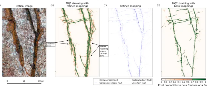
In Site A, we train two models MQ1 and MQ2 (training in the green zone in Figure 3a), the former with the refined ground truth map from the expert, the latter with the more basic ground truth map from the student. The scores of the models are then estimated in the validation zone of Site A, with respect to both the refined (TIR) and the basic mapping (TIB). The TI values (Figure 7) reveal that the model trained and validated with the refined mapping (MQ1) exhibits the best performance of the four realizations, with a TI of ∼0.62 against lower values (0.52–0.56) for the other models. Figures S9 and 8 visually confirm that, while both MQ1 and MQ2 predict the major faults well, their continuity is best revealed in MQ1, which also recovers a greater number of short faults present in the refined ground truth. MQ1 actually provides a rich fault mapping that well represents the complexity of the dense fracturing and faulting observed in the raw image. The predic-tions are so detailed that the en echelon fault patterns, the small relay zones between faults and the intense fracturing in inner damage zones are well recovered (Figure S9b), while they are not or much less in the MQ2 predictions (Figure S9e).
Therefore, training the model with a “basic quality” mapping is sufficient to properly recover the principal fractures and faults. However, training the model with more accurate and higher resolution mapping is necessary to allow it to perform richer predictions.
4.4. Reference Model
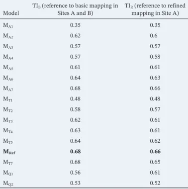
The scores of all the models calculated in the previous sections are presented in Table 2 and Figure 7. We remind the reader that the slightly slower TIR values mainly result from the training being made on basic mapping, thus at a lower resolution than the refined map used for the TIR calculation. The results demonstrate that, while most models provide reasonable results (most have a TI ≥ 0.55), the reference architecture MRef described in Section 3 provides the most accurate predictions (along with MA7, yet see Figure S5 for its lower prediction capacities). Therefore, in the following, we use the reference model MRef.
Figure S10 shows the standard ROC curve for all the models. The ROC curves are evaluated with the basic mapping in Sites A and B (Figures S10a and S10b) and also with the refined mapping in Site A (Figure S10c).
In keeping with prior findings, the models trained with the smallest data sets (MT1 and MT2) have the lowest scores, while MRef and MT7 (largest training data set) have the highest True positive rates at all False positive rates, hence are the most performant models.
Figure 7. Scores of all calculated models. See text for description of the different models. All models but MQ1 were
trained with basic mapping (in both Sites A and B for all models but MQ2). Tversky index TIB in green is calculated
with reference to basic mapping in both Sites A and B (averaged values), while TIR in blue is calculated with reference
to refined mapping in Site A only. MQ1 and MQ2 models were trained with refined and basic mapping, respectively, in
Site A only. The Tversky index in gray are calculated with respect to basic mapping. MRef provides the highest score,
especially with respect to basic mapping.
Figure 8. Impact of training data quality. (a and c) as in Figure 5. (b and d) show MRef predictions when MRef is trained with refined and with basic mapping,
respectively (in Site A only). Clearly, training the model with more accurate and higher resolution ground truth allows it to predict more significant tectonic features and to provide greater details on these features. See for instance the finer details in the architecture of the inner damage zone of the fault branch to the right, and in the segmentation and arrangements of the fault traces.
The calculations were done using a NVIDIA GeForce GTX 1080 GPU with 8 GB available memory. With 64 filters, a model is trained over one epoch in about 9 min. As we run the model up to 44 epochs (Figure S2a), MRef was generally calculated in ∼6 h (though 10–12 h are needed to ex-amine overfitting). Decreasing the number of filters to 32 decreases the training time by a factor of ∼3, making the prediction calculated in ∼2 h.
5. Detailed Evaluation of Reference Model Fault
Predictions
In the following sections, we evaluate the performance of the reference model Mref in more detail. Specifically, we examine its predictions for op-tical images from Sites A and B, and for previously unseen data of the same type and of different types (drone photography and optical satellite data).
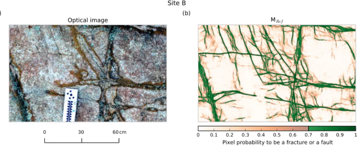
5.1. Results in Sites A and B 5.1.1. Site A
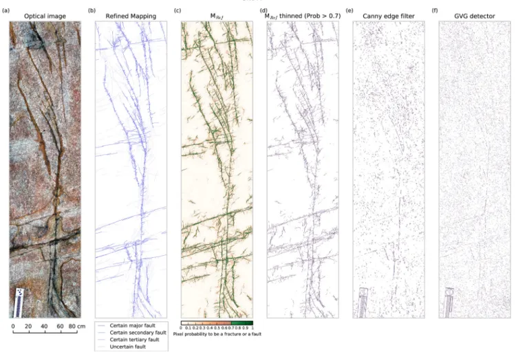
Figure 9 shows the MRef model results in the validation zone of Site A, and compares them to the raw optical image and the refined ground truth fault map. A zoomed view was shown in Figure 5d. The range of probabilities of the predictions is shown as a color scale. In Figure 9, the predictions are also shown as “thinned lines” (see explanation below), and compared to the results obtained with the Canny edge filter and the GVG detector.
We observe that the predictions of the CNN MRef model compare favora-bly to the manual mapping, revealing both the main fault traces and the secondary faults. Furthermore, most fractures and faults labeled as uncertain by the expert are recognized by the model. By contrast, the two edge detectors fall short to detect the actual faults and fractures in the images. Even the main fault traces are not well recovered by these algorithms, and there is no continuity in the fault traces: they are split into numerous small, isolated segments. In the results given by the CNN MRef model the continuity of the faults and fractures is much better preserved.
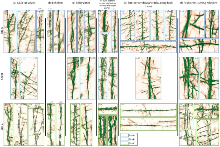
The model results reveal the tectonics of the site with great richness (Figure 9; enlargements provided in Figure 10). While the model does not provide any interpretation, a fault expert can see that the general ar-chitecture of the central ∼“N-S″ fault system is well recovered, showing the main fault trace splaying into long, oblique secondary faults at both tips. Another fault set, trending ∼“ENE,” is also well revealed. The architecture of smaller faults is likewise well depicted, with the model predicting remarkably well their tip splays (Figure 10a), their en echelon arrangement (Figure 10b), the relay zones between faults or segments (Figure 10c), the small bends in fault traces (Figure 10), the strongly oblique fracturing in between overlap-ping segments (Figure 9), and the dense sub-parallel fracturing forming inner damage either sides of major fault traces (Figure 10d). From the geometry of the en echelon arrangements and pull-apart type-relay zones along the ∼”N-S to NW-SE”-trending faults, we infer that the latter have a right-lateral component of slip. Although evidence is less numerous along the ∼”ENE”-trending faults, a few relay zones and en echelon dispositions suggest that these faults also have a right-lateral component of slip. That the two fault families have a similar slip mode suggest they are not coeval. Actually, although there is still ambiguity, sev-eral lines of evidence in both the refined map and the model predictions suggest that the ∼“N-S to NW-SE” faults cross-cut the ∼“ENE” faults, and thus post-date the latter (Figure 10f). Finally, the model predictions also recover fairly well the sub-perpendicular very short cracks identified by the expert along most signifi-cant fault traces (Figure 10e). Analyzing further the tectonic significance of the results is beyond the scope of the study. However, we demonstrate here the amazing capacity of the model MRef to map fractures and faults as accurately as the expert, and even in greater details in some places.
Model TIB (reference to basic mapping in Sites A and B) TIRmapping in Site A) (reference to refined
MA1 0.35 0.35 MA2 0.62 0.6 MA3 0.57 0.57 MA4 0.57 0.58 MA5 0.61 0.61 MA6 0.64 0.63 MA7 0.68 0.66 MT1 0.48 0.48 MT2 0.58 0.57 MT3 0.62 0.61 MT4 0.63 0.61 MT5 0.64 0.62 MRef 0.68 0.66 MT7 0.68 0.65 MQ1 0.56 0.61 MQ2 0.53 0.52
Note. All models but MQ1 were trained with basic mapping. TIB is
calculated with reference to basic mapping in both Sites A and B, while TIR is calculated with reference to refined mapping in Site A only.
Table 2