HAL Id: hal-01990798
https://hal.archives-ouvertes.fr/hal-01990798
Submitted on 23 Jan 2019
HAL is a multi-disciplinary open access
archive for the deposit and dissemination of
sci-entific research documents, whether they are
pub-lished or not. The documents may come from
teaching and research institutions in France or
abroad, or from public or private research centers.
L’archive ouverte pluridisciplinaire HAL, est
destinée au dépôt et à la diffusion de documents
scientifiques de niveau recherche, publiés ou non,
émanant des établissements d’enseignement et de
recherche français ou étrangers, des laboratoires
publics ou privés.
Pre-mission InSights on the Interior of Mars
Suzanne E. Smrekar, Philippe Lognonné, Tilman Spohn, W. Bruce Banerdt,
Doris Breuer, Ulrich Christensen, Véronique Dehant, Mélanie Drilleau,
William Folkner, Nobuaki Fuji, et al.
To cite this version:
Suzanne E. Smrekar, Philippe Lognonné, Tilman Spohn, W. Bruce Banerdt, Doris Breuer, et al..
Pre-mission InSights on the Interior of Mars. Space Science Reviews, Springer Verlag, 2019, 215 (1),
pp.1-72. �10.1007/s11214-018-0563-9�. �hal-01990798�
an author's https://oatao.univ-toulouse.fr/21690
https://doi.org/10.1007/s11214-018-0563-9
Smrekar, Suzanne E. and Lognonné, Philippe and Spohn, Tilman ,... [et al.]. Pre-mission InSights on the Interior of Mars. (2019) Space Science Reviews, 215 (1). 1-72. ISSN 0038-6308
Pre-mission
InSights on the Interior of Mars
Suzanne E. Smrekar1· Philippe Lognonné2· Tilman Spohn3· W. Bruce Banerdt1·
Doris Breuer3· Ulrich Christensen4· Véronique Dehant5· Mélanie Drilleau2·
William Folkner1· Nobuaki Fuji2· Raphael F. Garcia6· Domenico Giardini7·
Matthew Golombek1· Matthias Grott3· Tamara Gudkova8· Catherine Johnson9,10·
Amir Khan7· Benoit Langlais11· Anna Mittelholz9· Antoine Mocquet11·
Robert Myhill12· Mark Panning1· Clément Perrin2· Tom Pike13·
Ana-Catalina Plesa3· Attilio Rivoldini5· Henri Samuel2· Simon C. Stähler7·
Martin van Driel7· Tim Van Hoolst5· Olivier Verhoeven11· Renee Weber14·
Mark Wieczorek15
Abstract The Interior exploration using Seismic Investigations, Geodesy, and Heat
Trans-port (InSight) Mission will focus on Mars’ interior structure and evolution. The basic struc-ture of crust, mantle, and core form soon after accretion. Understanding the early differ-entiation process on Mars and how it relates to bulk composition is key to improving our understanding of this process on rocky bodies in our solar system, as well as in other solar
B
S.E. Smrekar ssmrekar@jpl.nasa.gov1 Jet Propulsion Laboratory, California Institute of Technology, 4800 Oak Grove Drive, Pasadena, CA 91109, USA
2 Institut de Physique du Globe de Paris, Univ Paris Diderot-Sorbonne Paris Cité, 35 rue Hélène Brion – Case 7071, Lamarck A, 75205 Paris Cedex 13, France
3 German Aerospace Center (DLR), Rutherfordstrasse 2, 12489 Berlin, Germany 4 Max Planck Institute for Solar System Research, Göttingen, Germany
5 Royal Observatory Belgium, Av Circulaire 3-Ringlaan 3, 1180, Brussels, Belgium 6 Institut Superieur de l’Aeronautique et de l’Espace, Toulouse, France
7 Institut für Geophysik, ETH Zürich, 8092, Zürich, Switzerland 8 Schmidt Institute of Physics of the Earth RAS, Moscow, Russia 9 University of British Columbia, Vancouver, Canada
10 Planetary Science Institute, Tucson, AZ, USA
11 Laboratoire de Planétologie et Géodynamique, UMR-CNRS 6112, Faculté des Sciences et Techniques, Université de Nantes, Nantes, France
12 School of Earth Sciences, University of Bristol, Bristol, UK
13 Department of Electrical and Electronic Engineering, Imperial College, London, UK 14 NASA Marshall Space Flight Center, 320 Sparkman Drive, Huntsville, AL 35805, USA
systems. Current knowledge of differentiation derives largely from the layers observed via seismology on the Moon. However, the Moon’s much smaller diameter make it a poor ana-log with respect to interior pressure and phase changes. In this paper we review the current knowledge of the thickness of the crust, the diameter and state of the core, seismic attenua-tion, heat flow, and interior composition. InSight will conduct the first seismic and heat flow measurements of Mars, as well as more precise geodesy. These data reduce uncertainty in crustal thickness, core size and state, heat flow, seismic activity and meteorite impact rates by a factor of 3–10× relative to previous estimates. Based on modeling of seismic wave propagation, we can further constrain interior temperature, composition, and the location of phase changes. By combining heat flow and a well constrained value of crustal thickness, we can estimate the distribution of heat producing elements between the crust and mantle. All of these quantities are key inputs to models of interior convection and thermal evolution that predict the processes that control subsurface temperature, rates of volcanism, plume dis-tribution and stability, and convective state. Collectively these factors offer strong controls on the overall evolution of the geology and habitability of Mars.
Keywords Mars· InSight · Interior · Seismology · Heat flow · Geodesy · Crust · Mantle ·
Core
1 Introduction
The first step in planet formation is accretion of planetesimals. If accretion results in suffi-cient mass and energy to melt the initial body, all planetary bodies will differentiate into at least three compositional layers: the dense core at the center, an intermediate density man-tle, and a buoyant crust at the surface (Elkins-Tanton et al.2011). The precise thickness of these layers and details such as the state (molten and/or solid) of the core, the temperature of mantle, and any layering in the crust, contain important information about the processes that shape the overall evolution of a planet (Mocquet et al.2011). Processes such as magma ocean formation and overturn, convective style and lithospheric mobility all shape interior structure and thermal evolution. Global overturn models also make predictions about final crustal thickness. The key variables in models of crust formed via accumulation of melt products above a convecting mantle predict a large range of crustal thickness. The modeled production of crust via pressure release melting in a convecting mantle is strong function of temperature and volatile content. If present on early Mars, plate tectonics would have cooled Mars more rapidly than stagnant lid convection. The thickness and state of the mantle and core affect the geometry and heat loss rate of convection, and thus the history of volcanism and volatile outgassing.
The intermediate size of Mars between Earth and the Moon, the only two bodies for which seismic and heat flow data have been acquired to date, places it in the sweet spot for understanding early planetary formation. The Moon’s diameter limits the phase transitions in the interior to those occurring at relative shallow depths on Earth (Khan et al.2013; Kuskov et al.2014), thus limiting applicability to larger bodies. Mars is large enough to be in the same pressure regime as Earth’s upper mantle (Fig.1), small enough to be geologically arrested enough to preserve its original crust. Mars’ relatively small volume also means that it contains insufficient heat producing elements to maintain vigorous present day geologic activity, thus preserving much of its original crust. Additionally, there is a wealth of data for
Fig. 1 Interior structure of Earth, Mars and the Moon, with known phase transitions for Earth and possible
phase transition locations for Mars
Mars, including from both missions and meteorites, that provide strong constraints on its original composition and geologic evolution.
The InSight mission will provide the first seismic and heat flow data for Mars, enabling unprecedented constraints on interior structure and evolution. InSight launches in May of 2018, and arrives at Mars on November 26, 2018, landing on Elysium Planitia (Golombek et al.2017). The three primary instruments are the Seismic Experiment for Interior Structure (SEIS), the Heat Flow and Physical Properties Package (HP3), and the Rotation and Inte-rior Structure Experiment (RISE). SEIS consists of a set of 3 very broad band seismometers coupled with 3 short period seismometers (Lognonné et al.2018). Techniques for determin-ing interior structure with a sdetermin-ingle station are described in Panndetermin-ing et al. (2015), Böse et al. (2017). HP3is a self-hammering mole that deploys a tether with embedded temperature
sen-sors to a depth of 3–5 m, taking thermal conductivity measurements as it descends (Spohn et al.2018). RISE (Folkner et al.2018) uses two low gain X-band antennas to precisely track the lander location over a Martian year to determine the rotation of Mars, as well as its precession and nutation. RISE data will enable the first estimate of Mars’ nutation, thus providing tight constraints on core size, density and state (liquid versus solid). The lander Instrument Deployment Arm (Trebi-Ollennu et al.2018) will deploy SEIS and HP3on the
surface of Mars, with the aid of two cameras to image the deployment zone (Maki et al.
2018). Additionally, a pressure sensor, wind sensors, and a magnetometer are used to decor-relate seismic events from atmospheric effects or lander magnetic field variations (Banfield et al.2018). The HP3 experiment includes a radiometer to determine surface temperature variations (Spohn et al.2018). Finally, color images of the surface as well as experiments with the arm and scoop coupled with information from SEIS and HP will be used to bet-ter understand the geology and physical properties of the surface and shallow subsurface (Golombek et al.2018)
Using data from its three primary instruments, InSight will accomplish six science ob-jectives (Banerdt et al.2013):
– Determine the size, composition and physical state of the core – Determine the thickness and structure of the crust
– Determine the composition and structure of the mantle – Determine the thermal state of the interior
– Measure the rate and distribution of internal seismic activity – Measure the rate of impacts on the surface
Fig. 2 Key topographic features on Mars include the hemispherical dichotomy, separating the northern
low-lands from the southern highlow-lands, the Tharsis volcanic complex, and major impact basins, as labeled
In this paper, we will begin by summarizing the available constraints on the interior of Mars. We then describe the theoretical framework for models of the interior structure and thermal evolution including equations of state, convection models, and their interdepen-dence. Finally, we describe an approach to integrating the new constraints to be provided by InSight into a new framework for understanding early differentiation, core formation, dy-namo history, mantle mineralogy and volatile content, thermal evolution including dydy-namo history, and crustal formation processes.
2 Available Constraints on the Martian Interior
2.1 Geologic History
The geologic history of Mars provides key constraints on interior evolution. The crater-ing record shows that much of the crust formed very early in Martian history. Both the hemispheric dichotomy between the southern highlands and northern lowlands and the huge Tharsis volcanic complex provide important constraints on interior structure and evolution.
Impact crater density is used to divide the history of Mars into fours periods (see Werner and Tanaka 2011 for discussion and possible alternate dates): Pre-Noachian (> 4.1 Ga), Noachian (4.1–3.8 Ga), Hesperian (3.8–3.0 Ga), and Amazonian (< 3.0 Ga). Much of the crust is Hesperian or older, making Mars an ideal location to study initial crustal forma-tion. The largest impact basins have locally excavated the crust. The Hellas and Isidis basins are similar in size (see Fig.2), but have very different depths and gravity signatures due to subsequent filling of Isidis (Searls et al.2006). The largest basin, Utopia, is located in the northern plains and is completely buried. As discussed below, the entire northern hemi-sphere may have formed as a result of a very early impact, or via endogenic processes. High resolution topography revealed numerous impact basins buried under 1–2 km of fill in the northern plains, implying formation in the Pre-Noachian (Nimmo and Tanaka2005; Frey
2006). Younger, Amazonian age features consist of polar cap ice deposits, volcanism, sedi-ments, and impacts. The InSight landing site in Elysium Planitia, is located near some of the youngest volcanic and tectonic features on the planet (Vaucher et al.2009; Burr et al.2002), potentially providing seismic sources (Taylor et al.2013; Taylor2013). The most prominent topographic features are the dichotomy between the northern and southern hemispheres and
the Tharsis volcanic rise. Each of these features are clearly visible in the topography of Mars (Fig.2), and relate directly to interior processes or crustal structure.
The southern highlands are on average 4–5 km higher than the northern lowlands (Fig.2), and have a much higher crater density due to infilling of the northern plains by volcanism and sediments. The origin of dichotomy has been attributed to both endogenic processes such as hemispherical scale (degree 1) mantle convection (Schubert and Lingenfelter1973; Wise et al.1979a,b; Breuer et al.1997,1998; Zhong and Zuber2001) or very early plate tectonics (Sleep1994). Exogenic models include single (Wilhelms and Squyres1984) or multiple (Frey and Schultz1988) impact events. In some scenarios, a degree-1 plume formed under the southern hemisphere and caused massive melting that thickened the crust and produced higher elevation in the south via isostatic adjustment (Zhong and Zuber2001). Alternatively, a degree-1 plume may have thinned the crust in the northern lowlands (Roberts and Zhong 2006). Another proposed mechanism is the overturn of a buoyantly unstable mantle following magma ocean solidification (Elkins-Tanton2008). Andrews-Hanna et al. (2008) proposed that the northern plains were formed via a single impact that created an elliptical basin, as predicted by modeling (Marinova et al.2008). They used both gravity and topography to remove the signature of Tharsis and Arabia Terra on the shape of the northern plains.
These models have different implications for the composition and structure of the interior. A major question has been whether there is a difference in crustal composition between the north and the south that contributes to the difference in elevation. A recent investigation of the northern lowlands basement composition, as revealed by impact crater excavations, finds a range of hydrated minerals beneath the surficial volcanic fill, similar in composition to those found in the southern highlands (Pan et al.2017). Although the sampling depth is limited, this work strongly suggests that the difference in elevation reflects a difference in crustal thickness rather than composition. Another puzzling question is why the northern lowlands exhibit very little crustal remanent magnetization relative to the southern highlands despite their similarity in age (Langlais et al.2004). One possible explanation is that the dynamo on Mars was asymmetric (Stanley et al.2008).
Mars’ other major physiographic feature is the Tharsis rise, a massive volcanic complex. It covers one quarter of the Martian surface and is the largest volcanic construct in the solar system (Fig.2). The rise itself is 10 km high, with three central volcanoes with heights of
>10 km each, in addition to Olympus Mons to the northwest and Alba Patera to the north (Fig.2). This huge feature affects the global topography, gravity, and surface deformation (see Golombek and Phillips2009, for a review). The age of the planetary scale deformation associated with Tharsis and the extensive volcanism indicate that the region has been active over most of the age of Mars. Although much of the topography is interpreted to have formed early in Martian history, modest volcanism persisted into the Amazonian. For example, Arsia Mons may have been active as recently as 10–90 Ma (Richardson et al.2017).
The massive topography of Tharsis must be held up by some combination of composi-tional and/or thermal isostasy, flexure, and dynamic mantle support. The exact proportion and origin of these mechanisms have implications for interior structure, mantle dynamics, and thermal evolution. Models of loading of the lithosphere in response to Tharsis volcan-ism show that membrane stresses are capable of supporting the majority of the load (Banerdt et al.1982,1992) and successfully predict more deformation features than isostatic models, even if coupled with a regional stress field (Tanaka et al.1991). Much of the lithospheric de-formation dates to the Middle Noachian (> 3.8 Ga), and requires that the Tharsis load have the dimensions of the current topographic rise (Phillips et al.2001). Modeling of the present-day gravity and topography fields also predict the pattern of deformation, indicating that the
stress fields have largely been unchanged since the Noachian (Banerdt and Golombek2000). Bouley et al. (2016) proposed an alternative explanation, suggesting that the orientation of a key deformation feature, valley networks, can be explained by topographic gradients be-tween the northern and southern hemispheres prior to Tharsis formation. In this scenario, major Tharsis construction begins in the Late Noachian. One question for these loading models and interior structure is the degree of support due to low density mantle residuum (Phillips et al.1990).
The Tharsis rise has been interpreted as forming over one or more mantle plumes. The scale of plume, the formation of most of the volcanism early in Martian history, and the con-tinuation of volcanic activity into recent Martian geologic history, have posed a challenge for convection simulations. A series of convection models have shown that the presence of a phase transition near the core-mantle boundary supports the formation of a small number of plumes and areal concentration of plumes (Harder1998,2000; Harder and Christensen
1996; Breuer et al.1998). The size of the core is the dominant factor in determining whether or not phase transitions near the core-mantle boundary are present, and thus the applicabil-ity of such plume models. Another key challenge is for the convection pattern to localize rapidly enough to be consistent with timing constraints on the formation of Tharsis. A key question is source of relatively recent volcanism given the very thick lithosphere under Thar-sis. Modeling suggests that if present, a plume or other buoyant region at depth contributes only modestly to support of the topography (Lowry and Zhong2003; Zhong and Roberts
2003; Roberts2004; Redmond and King2004). Alternative ideas for the formation of Thar-sis include warming of the mantle (Solomon and Head1982a). Warming might occur under a thick, insulating southern hemisphere crustal layer (Wenzel et al.2004).
2.2 Composition
Our current knowledge of the bulk chemical and mineralogical composition of Mars is based on the analysis of the Martian meteorites, remote sensing and in-situ analysis of the Martian surface as well as on geophysical properties of the planet.
2.2.1 Meteorites, Remote Sensing and In-Situ Analysis
Martian meteorites partially referred to as SNC meteorites (shergottites, nakhlites, and chas-signites) are igneous rocks of varying mafic to ultramafic igneous lithologies. The meteorites exhibit both intrusive and extrusive textures including: basalt and lherzolite (shergottites), orthopyroxenite (ALH 84001), clinopyroxenite (nakhlites), and dunite (Chassigny). Except for ALH 84001, a 4.5-Ga sample of the Noachian crust, all SNCs were extracted from Ama-zonian volcanic terrains. The most representative samples are the shergottites that show crystallization ages between 170 and 600 Ma (e.g., McSween and McLennan 2013). For characterizing the chemistry and mineralogy of igneous materials at the surface of Mars, remote sensing data are also available. Mineralogical information is generally obtained us-ing the visible and infrared range of the electromagnetic spectrum (Bandfield et al.2000; Poulet et al.2009), whereas abundances of chemical elements are principally derived from gamma-rays (Boynton et al.2007) and neutron spectroscopy (Feldman et al.2011). In gen-eral, the spectral analysis of the Martian surface does not provide a good match to the spec-tral signature of the SNC meteorites (Hamilton et al.2003; Lang et al.2009) and Martian meteorite-like lithologies represent only a minor portion of the dust-free surface. However, the distinctive mineralogical characteristics of SNCs (ferroan olivine and pyroxenes, sodic plagioclase) are commonly indicated by remote-sensing data. Igneous rocks have also been
analyzed in-situ in Gusev Crater (e.g., Squyres et al.2004). These rocks also range from basaltic to cumulate rocks (e.g., Dreibus et al.2007; McSween et al.2006; Ming et al.2008; Squyres et al.2008) but are much older (∼ 3.65 Ga) than shergottites (Arvidson et al.2003; Greeley et al.2005) and have significantly different chemistry than basaltic shergottites (Fil-iberto et al.2006; McSween et al.2009; Taylor et al.2006). These findings challenge the use of the SNCs in defining diagnostic geochemical characteristics and in constraining com-positional models for Mars. We also note that extensive sedimentary deposits composed of phyllosilicates and sulfates have been observed from orbit and by rovers in Gale crater and Meridiani Planum, but spectral data from orbit (Ehlmann et al.2011; Ehlmann and Edwards
2014) and chemical and mineralogical data from the surface (Davis et al.2005; Grotzinger et al.2014) show that most are basaltic in composition or have been altered from an initial basaltic composition, indicating that the martian crust is basaltic in composition.
2.2.2 Bulk Composition
Geochemical Perspective Assuming that the SNC meteorites are representative of the Martian crust, models based on geochemical arguments (Dreibus and Wänke1984,1985; Wänke et al. 1994; Lodders and Fegley 1997; Morgan and Anders 1979; Sanloup et al.
1999; Mohapatra and Murty2003) have been developed to estimate the composition of the bulk silicate portion of Mars (see Taylor2013, for a recent review). To derive the chemical composition of Mars from the chemical compositions of the Martian meteorites, two general approaches have been applied. The first approach uses the elemental correlations in the Martian meteorites, assuming that refractory elements are present in chondritic abundances (Dreibus and Wänke1984,1985; Wänke et al.1994; Halliday and Porcelli2001; Longhi et al.1992; Taylor2013) whereas the second approach uses oxygen isotope systematics of the SNC meteorites and match them via mass balance equations to mixtures of different chondritic material (Lodders and Fegley1997; Sanloup et al.1999; Burbine and O’Brien
2004). Table1shows a compilation of 5 different models of the bulk composition of Mars. These compositions represent the primitive mantle of Mars, i.e., unaffected by magmatic processes such as magma ocean fractional crystallization and crust formation.
All compositional models share the characteristic that the Martian mantle is more Fe-rich than the Earth, consistent with the Fe-rich compositions of SNC meteorites. The significant difference between oxygen isotope-based and element-based estimates is the strong enrich-ment in volatile eleenrich-ments in the isotope models. This enrichenrich-ment is not seen in the GRS data (Taylor et al.2006) for which K/Th is 5300 for the Martian surface versus K/Th 16400 in the study of Lodders and Fegley (1997). The model by Wänke et al. (1994), recently reassessed by Taylor (2013) using a larger meteoritic record, is broadly consistent with the surface K/Th ratio measured by the GRS instrument (Taylor et al.2006) and is currently the most widely accepted compositional model.
It should be noted that although Martian meteorites are an important data set, element abundances in the crust derived from in-situ and remote sensing measurements suggest that magma source regions are heterogeneous and constraints on mantle compositional models from the meteorites may not apply to the entire mantle. In addition, the isotope character-istics of the SNCs indicate the formation of several reservoirs, which have formed rapidly in the first ten million years after the formation of the planet and have not been mixed since then (e.g., Mezger et al.2013). An aspect that is difficult to take into account in current mod-els of internal structure, since the size and location of these reservoirs are unknown—thus typically a chemically homogeneous mantle is assumed.
Table 1 Bulk Martian crust and
mantle (primitive mantle) and core composition for model MA (Morgan and Anders1979), DW (Dreibus and Wänke1984; Wänke et al.1994), LF (Lodders and Fegley1997), SA (Sanloup et al.1999) and TA (Taylor2013)
MA DW LF SA TA
Bulk crust & mantle composition (wt.%) in major oxides
SiO2 41.59 44.4 45.39 47.79 43.7 Al2O3 6.39 3.02 2.89 2.52 3.04 MgO 29.77 30.2 29.71 27.46 30.5 CaO 5.16 2.45 2.36 2.01 2.43 Na2O 0.1 0.5 0.98 1.21 0.53 K2O 0.01 0.04 0.11 – 0.04 TiO2 0.33 0.14 0.14 0.1 0.14 Cr2O3 0.65 0.76 0.68 0.7 0.73 MnO 0.15 0.46 0.37 0.4 0.44 FeO 15.85 17.9 17.21 17.81 18.1 Core composition Fe 88.1 77.8 81.1 76.6 78.6 Ni 8 7.6 7.6 7.2 S 3.5 14.2 10.6 16.2 21.4
Geophysical Perspective Geophysical analyses typically rely on results obtained from the geochemical studies to predict the geophysical response of these models. In particular, many of the geophysical and experimental approaches are based on the Dreibus and Wänke (1984) model composition with the purpose of determining mantle mineralogy (Bertka and Fei1997,1998). Combined with equation-of-state (EOS) modeling allows for determination of a model density profile that can used for making predictions and be compared to observa-tions (e.g., mass, moment of inertia, and tidal response). Many numerical approaches have also been conducted (Longhi et al.1992; Kuskov and Panferov1993; Mocquet et al.1996; Sohl and Spohn1997; Sohl et al.2005; Verhoeven et al.2005; Zharkov and Gudkova2005; Khan and Connolly2008; Rivoldini et al.2011; Wang et al.2013; Khan et al.2018). These studies are based on forward/inverse modeling of the available geophysical observations us-ing either parameterized phase diagram or phase equilibrium computations. These studies generally concur with the geochemical evidence for an Fe enriched Martian mantle relative to Earth’s magnesian-rich upper mantle (McDonough and Sun1995).
2.2.3 Mineralogy of the Reference Models
The major mineralogical constituents of the mantle are those expected for an Earth-like planet: olivine, ortho- and clino-pyroxenes, and garnets, but in different proportions among the proposed models (Dreibus and Wänke1985; Sanloup et al.1999; Taylor2013; Bertka and Fei1997) (Fig.3). These models show that (1) olivine undergoes phase transitions: to wadsleyite around 12–13 GPa and to ringwoodite at 14–16 GPa; and (2) that pyroxenes pro-gressively transform into garnet solid solutions at depth. The sharpness and the location of these mineralogical transformations mainly depend on the iron enrichment and temperature of the mantle with exothermic transformations occurring at shallower depths in the case of hotter areotherms. Compared to standard Earth-like mantle compositions (e.g., a pyrolitic one), Mars’ mantle mineralogy is characterized by the existence of orthopyroxenes over a large range of pressure (up to 10 GPa), followed by high-pressure clinopyroxene phases
Fig . 3 Modal m ineralogy of Mars as a function o f p ressure for four b u lk compositions. (a ) O li vine-rich composition o f D reib us and Wänk e ( 1985 ) re v ised by T aylor ( 2013 ); (b ) Pyrox ene-rich composition o f Sanloup et al. ( 1999 ); (c ) M odal composition synthetized by Bertka and Fei ( 1997 ) at h igh p ressure and h igh temperature. T he iron content o f the three Martian m odels (Fe#0.2) is twice the Earth’ s m antle v alue (Fe#0.1). A n E arth-lik e p yrolitic composition (Ringw ood 1975 ) is d isplayed in panel (d ) for comparison
that co-exist with their low-pressure counterparts and with wadsleyite between 10 GPa and 15 GPa.
The existence of a lower mantle as in the Earth is highly dependent on physical conditions at the core-mantle-boundary (CMB), core size and Fe-content. The stability of these silicates is strongly sensitive to temperature and pressure conditions at the CMB: a large core results in either a thin or no lower mantle, whereas higher temperatures will stabilize bridgmanite at lower pressures. Compositionally, small cores will tend to be Fe-rich and favor presence of a lower mantle whereas large cores will tend to be enriched in light elements and inhibit a lower mantle (e.g., Khan et al.2018).
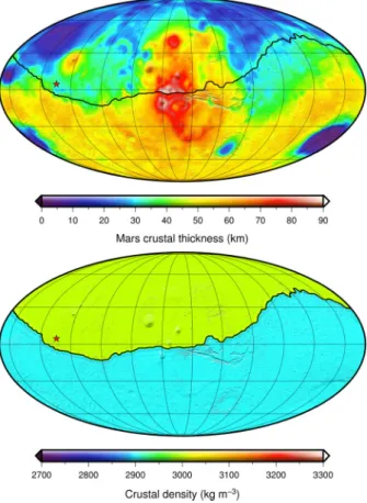
2.3 Gravity, Topography, and Crustal Thickness
Models of the gravity field of Mars have been improved successively by the analysis of ra-dio tracking data from multiple spacecraft over a time span of several decades. The most recent models (e.g., Genova et al.2016; Goossens et al.2017) are expressed up to spherical harmonic degree and order 120, which corresponds to a full-wavelength spatial resolution of about 178 km on the surface. The gravity field is uniquely determined by the three-dimensional distribution of mass within the planet, and thus provides information on how density varies both laterally and with depth. Interpretation of the gravity field is well known to be inherently non-unique, but by making reasonable assumptions based on geologic ex-pectations, and by making use of the surface topography of the planet (Smith et al.2001) as a constraint, it is possible to invert for several properties related to the crust and lithosphere. One analysis approach is to assume that Mars differentiated into a distinct crust and mantle, and that the ancient highland crust is isostatically compensated. This model pre-dicts a relationship between the average crustal thickness, the crustal density, and the ratio of the geoid and topography (Wieczorek and Phillips1997). Mars is divided along a hemi-spheric dichotomy into the heavily cratered southern highlands and the northern lowlands, where impact basins have been buried by a combination of sedimentation and volcanism. Wieczorek and Zuber (2004) argue that the southern highlands are more likely to be iso-statically compensated than the lowlands. They find that the best-fitting average thickness of the highlands crust was between 53 and 68 km for assumed crustal densities of 2700 and 3100 kg m−3, respectively. When considering the uncertainties on the geoid-to-topography ratio, the 1σ limits of the average crustal thickness range from 39 to 81 km. The major uncertainty with this approach is that it is difficult to prove that the ancient crust is in fact isostatically compensated, and the density of the crust is highly uncertain.
A second modeling approach that can be made is to assume that the rigid outer portion of the planet, the lithosphere, behaves as an elastic shell when subjected to loads both on the surface and within the crust. For a given elastic thickness, these models compute the loads and lithospheric deflections that match the observed surface topography. Though these models depend upon several parameters, including the crustal thickness and mantle density, the density of the surface load is the best constrained. Localized spectral analyses applied to the large Martian volcanoes shows that the densities of the volcanic loads are close to 3200 kg m−3 (McGovern et al. 2004; Belleguic et al.2005; Grott and Wieczorek2012; Beuthe et al.2012), which are consistent with the densities of the Martian basaltic meteorites (Neumann et al. 2004). Only for the Elysium rise is the density of the crust beneath the volcanic load constrained in these models. For this region in the northern lowlands, the density of the underlying crust was found to be the same as that of the volcanic load itself (Belleguic et al.2005), suggesting that the entire northern lowland crust may be largely basaltic. The elastic thicknesses obtained from these studies will be discussed in Sect.2.4.
A third modeling approach is to assume that the observed gravitational field is a result of variations in relief along the surface and crust-mantle interface. By assuming densities of the crust and mantle, as well as a mean thickness of the crust, it is possible to invert for the relief along the crust-mantle interface, providing a global crustal thickness map (e.g., Neu-mann et al.2004). This modeling approach makes no assumptions as to whether the crust is isostatically compensated or not, and in practice, the parameter values for the inversions are constrained such that the minimum crustal thickness is equal to a specified value that is greater than zero. The minimum crustal thickness of Mars is found to be located in the inte-rior of the Isidis impact basin, which lies just south of the dichotomy boundary. One of the major uncertainties with these models is that the crustal density is not known. As shown by Baratoux et al. (2014), the surface composition of Mars is similar to the basaltic meteorites. If these high densities are representative of the underlying crust, to obtain positive crustal thicknesses everywhere, the mean crustal thickness could be as high as 110 km (see also Pauer and Breuer2008, who provide a maximum density of 3020 kg m−3). The minimum crustal thickness to use in these models is also unconstrained, though a value close to zero, as with the Moon (Wieczorek et al.2013; Miljkovi´c et al.2015), is probably a reasonable estimate. Lastly, it is likely that the density of the subsurface crust varies laterally, but these variations are not easy to constrain based on remote sensing data.
We have constructed a suite of crustal thickness models for use in modeling the seismic data that will be obtained from InSight (see also Plesa et al. 2016). These models differ from previous studies in several ways. First, in computing the gravity field, we consider the hydrostatic deflection of density interfaces within the mantle and core using the reference density models shown in Sect.3.2.3. These models consider the non-hydrostatic gravita-tional potential arising from the lithosphere when computing the hydrostatic interfaces, and these deflections are responsible for 3.6–5.6% of the observed zonal degree-2 gravitational field. Second, we consider the possibility that the density of the crust in the northern low-lands is different from that of the southern highlow-lands (e.g., Belleguic et al.2005). Third, we consider a wide range of crustal densities, from 2700 to 3200 kg m−3. Lastly, as their are yet no seismic constraints on crustal thickness, we use a minimum thickness constraint, where the minimum crustal thicknesses from 1 to 20 km. The thickness of the crust at the InSight landing site varies from 19 to 90 km in these models. In Fig.4, we show one such model where the crustal densities of the southern highlands and northern lowlands are 2900 and 3000 kg m−3, respectively. Data obtained from the InSight mission will constrain the crustal thickness at the InSight landing site, and will also constrain the core and mantle density profiles.
2.4 Constraints on the Lithosphere Thickness
In the absence of direct heat flow measurements, temperatures in the planetary interior can be estimated from the mechanical properties of lithospheric plates. In this regard, the ef-fective elastic lithosphere thickness Te is commonly used to describe the response of the lithosphere to loading, and given a rheological model, the mechanical thickness of the litho-sphere Tm can be derived from Te. Using the yield-strength envelope formalism (McNutt
1984), Tm can in turn be identified with an isotherm, and in this way estimates of planetary heat flow can be derived.
Most Te estimates for Mars have been derived from gravity and topography admittance modeling (McGovern et al.2004; Kiefer2004; Belleguic et al.2005; Hoogenboom and Sm-rekar2006; Wieczorek2008; Grott and Wieczorek2012), but some geological features allow for more direct approaches. Phillips et al. (2008) have modeled the lithospheric deflection
Fig. 4 Representative crustal
thickness model (top) using the interior density profile for the model DWTh2Ref1. The crustal densities for the southern highlands and northern lowlands (bottom) are 2900 and 3000 kg m−3, respectively. The minimum crustal thickness was constrained to 1 km, which determines the average crustal thickness to be 42 km and the crustal thickness at the InSight landing site (star) to be 32 km. Data are presented in Mollweide projections centered over the Tharsis province (100◦W), and grid lines are spaced every 30 in latitude and longitude. The dictomomy boundary used in the lower image is taken from Andrews-Hanna et al. (2008)
due to polar cap loading, and analysis of rift flank uplift has been used to constrain Te at the Tempe Terra, Coracis Fossae, and Acheron Fossae rift systems (Barnett and Nimmo2002; Grott et al.2005; Kronberg et al.2007). In addition, the lithospheric stress distribution due to mascon-loading at the Isidis basin has been employed to model Te using the position of the Nili Fossae circumferential graben system as model constraint (Comer et al.1985; Ritzer and Hauck2009). Other approaches estimate Te from an analysis of the depth to the litho-sphere’s brittle-ductile transition (Schultz and Watters2001; Grott et al.2007; Ruiz et al.
2009; Mueller et al.2014; Egea-Gonzalez et al.2017), but these approaches carry additional uncertainty.
To correlate heat flow estimates with time it is usually assumed that the observed paleo-flexure corresponds to the age of the deformed surfaces, and paleo-flexure is generally assumed to be frozen-in at the time of loading. However, care must be taken when interpreting these results, as stresses in the lithosphere will decay as a function of time due to viscous relax-ation and the true time corresponding to the observed paleo-flexure is generally determined by a competition between loading rate, lithospheric cooling rate, and stress relaxation rate (Albert et al.2000; Brown and Phillips2000). In this regard, the elastic thickness estimate by Phillips et al. (2008) is an exception, as the time of loading by the Martian polar caps can be tightly constrained to < 5 Myr (Phillips et al.2008).
Elastic thickness has increased with time (Golombek and Phillips2009; Grott et al.2013; Ruiz2014). In the Noachian, Te was < 20 km. Values quickly increased to > 50 km during the Hesperian, which can at least partially be attributed to rheological layering (Burov and
Diament1995; Grott and Breuer2008,2009). During the Amazonian Te further increased to 40 < Te < 150 km on average, and best estimates for the present-day elastic thickness are above 150 km. In particular, the absence of lithospheric deflection due to loading at the north polar cap locally constrains present-day Te to values greater than 300 km at this location (Phillips et al.2008). Such large present-day elastic thickness values could either imply a sub-chondritic bulk composition in terms of heat producing elements (Phillips et al.
2008), or a large degree of spatial heterogeneity of the mantle heat flow (Phillips et al.2008; Grott and Breuer2009,2010; Kiefer and Li2009; Plesa et al.2016; Breuer et al.2016). It is worth noting that some studies assume that the large Te determined for features on the Tharsis rise are representative for the rise itself (Banerdt and Golombek2000; Phillips et al.
2001). As a consequence, Te would have been much larger and close to 100 km during the Noachian (Zhong2002; Zhong and Roberts2003), and regional and global flexure models using Te= 100 km were found to be consistent with the location and orientation of tectonic features (Banerdt and Golombek2000) and valley networks (Phillips et al.2001).
2.5 Geodesy
Planetary geodesy is one of the primary means for probing the interior structure of planets, in particular when no seismic observations are available. By radio tracking many space-craft orbiting Mars, an accurate gravity field has been determined over the past decades. Expressed in terms of spherical harmonics, the field is now accurate up to about degree 100 (Konopliv et al.2016; Genova et al.2016), corresponding to a horizontal surface resolution of about 215 km. Most important for the deep interior of Mars are the lowest degrees. The degree-two components of the gravity field are related to the three principal moments of inertia of Mars, and as such inform on the mass distribution in the planet. Information on the radial density profile can be obtained from the mean moment of inertia, but this quantity cannot be determined from the gravity field alone. By complementing the degree-two com-ponents of the gravity field with precession, the mean moment of inertia of Mars has been determined and as such a first constraint on the overall mass distribution inside Mars from center to surface has been obtained.
Precession is determined from analysing radio tracking data of Martian landers and or-biters over several decades (e.g., Konopliv et al.2011; Le Maistre2013; Kuchynka et al.
2014; Konopliv et al.2016). The most recent estimate of the precession rate of Mars yields a mean moment of inertia normalized by the product of mass and squared radius of Mars of 0.3639±0.0001, with the error mainly due to the error on the precession estimate (Konopliv et al.2016). Since it is an integrated quantity over the mass density in Mars, the moment of inertia, even when accurately known, cannot precisely constrain more local properties of the interior such as for example the radius of the core. Even employing the simplifying assumption that Mars were to consist of two equal density layers (the core and the man-tle plus crust), the error on the core radius from the moment of inertia constraint would be several hundred km (Van Hoolst and Rivoldini2014). RISE will improve the determination of the precession rate by a factor of two but its effect on the estimate of the core radius is negligible without considering other data. Up to now, solar tides have been the most con-straining geodesy quantity for the core of Mars. Since the tidal potential is accurately known (Van Hoolst et al.2003), the tides can be interpreted in terms of the reaction of Mars to the gravitational forcing which is very sensitive to the size of a liquid core. Tidal surface dis-placements have not yet been observed since their amplitude is only a few centimeters at most (Van Hoolst et al.2003), but the mass redistribution inside Mars associated with tidal deformations has an observable effect on the orbital motion of spacecraft around Mars. The
Fig. 5 Core radius as a function
of Love number k2for the hot (solid curves) and cold (dashed curves) mantle temperature profile from Panning et al. (2016). The blue shaded area represents the range of k2values from Konopliv et al. (2016) and Genova et al. (2016). The acronyms stand for the different mantle mineralogy models DW: (Taylor2013), EH45: (Sanloup et al.1999), LF: (Lodders2000), MM: (Mohapatra and Murty 2003), MA: (Morgan and Anders 1979). Models agree at 1σ with the average moment of inertia of Mars (MOI= 0.3639 ± 0.0001) (Konopliv et al.2016)
tidally induced changes in the external gravitational potential of Mars are described by the Love number k2. The most recent determination of the solar tides yields k2= 0.163 ± 0.008,
based on the estimates of Konopliv et al. (2016) and Genova et al. (2016). It implies that the radius of the core is about 1788± 73 km for the SEIS reference models (see Fig.5).
The radio science experiment RISE of InSight will improve the estimate of precession and thus of the moment of inertia of Mars, but more importantly it will for the first time measure the effect of the core on the periodic orientation changes of Mars in space (nuta-tions). This will allow determining the dependence of nutation on the interior structure. In particular, it will be able to improve our knowledge on the core (see the paper of Folkner et al.2018, in this issue).
2.6 Crustal Magnetization and Dynamo History
Mars has no present dynamo field but Mars Global Surveyor (MGS) data revealed a rema-nent crustal magnetic field that provides constraints on crustal evolution and thermal history, in particular on the existence and timing of an ancient dynamo. There are also time-varying fields, driven by interaction of the Interplanetary Magnetic Field (IMF) with the magnetic field of Mars. They induce electrical currents in the interior that result in secondary induced fields. Magnetic sounding techniques use such time-varying magnetic fields at different pe-riods to probe the interior electrical conductivity structure as a function of depth. Below we discuss Mars’ crustal field and its implications for Mars’ thermal history. Magnetic sounding and electrical conductivity structure are discussed in Sect.3.3.3.
2.6.1 The Crustal Magnetic Field: Observations and Models
Systematic mapping of the martian magnetic field has been conducted by MGS (1997–2006) and MAVEN (Mars Atmosphere and Volatile EvolutioN, 2014–present), both of which mea-sure the vector magnetic field. MGS collected data mainly at 360–440 km altitude in a 2 am/2 pm orbit. Observations below 360 km were made over about 20% of the surface but
mostly on the dayside (magnetically noisier). MAVEN is in a highly eccentric orbit with periapsis covering a range of local times and latitudes, typically at 140–170 km altitude, but occasionally lowered to about 110 km.
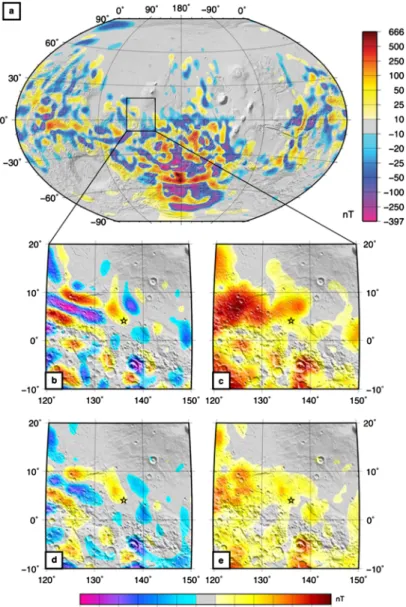
The first crustal magnetic field maps were of data shown at satellite altitude (Acuña et al.1999,2001; Connerney et al.2001). Early global models represented the magnetic field either using equivalent source dipoles (e.g., Purucker et al.2000; Langlais et al.2004) or spherical harmonics (e.g., Arkani-Hamed2001,2002,2004; Cain2003); for a detailed review see Langlais et al. (2010a). Early interpretations, largely based on high-altitude measurements, indicated possible relations with tectonics patterns or signatures (Conner-ney et al.1999; Nimmo and Stevenson2000; Connerney et al.2005), with long, east-west aligned, magnetic field anomalies in the southern hemisphere. These were later challenged by more recent models and lower altitude maps (e.g., Ravat2011). They include a spheri-cal harmonic description of the field with a spatial resolution of 195 km, that is stable with respect to downward continuation to the planetary surface (Morschhauser et al.2014) and a locally higher resolution model over the martian South Pole (Plattner and Simons2015). Electron reflectometer observations by MGS have also been used to build maps of the crustal magnetic field strength at 170 km latitude (Lillis et al.2008), and combined with vector data (Langlais et al.2010b). Crustal field models differ in details, some of which may be impor-tant to interpretations (see later), but all have the same major features. The strongest fields are spatially associated with the pNoachian-age Terra Cimmeria and Terra Sirenum re-gions, crustal fields are notably absent or weak in many major impact basins and over the smoother terrain north of the hemispheric dichotomy (see Fig.6).
The maximum spatial resolution achievable by magnetic field models depends primarily on the minimum altitude of nighttime (quiet) data. Recent MAVEN data show previously unresolved signals, especially at altitudes below 250 km. They permit higher spatial resolu-tion crustal field models, both because of the substantial increase in low altitude, nighttime observations and because they allow MGS measurements to be better selected by cross val-idation (Mittelholz and Johnson2016; Langlais and Thebault2017).
2.6.2 Implications for Crustal Structure and Mars’ Thermal Evolution
The strong magnetic anomalies imply large volumes of magnetized crust and/or strong mag-netizations (Connerney et al. 1999; Purucker et al.2000) acquired in an ancient dynamo field. Major, coupled questions arise, which are listed below.
(1) How was the magnetization acquired? The canonical interpretation of the martian mag-netic anomalies is that they arise from thermal remanent magnetization (TRM), acquired during cooling of crustal rocks (either new melts or reheated crust) in the presence of a global field. Another possibility is shock remanent magnetization (SRM) which has been inferred for pyrrhotite-dominated shergottite meteorites (Gattacceca and Ro-chette2004), and shock can also result in demagnetization signatures (Hood2003). Fi-nally, chemical remanent magnetization (CRM) due to alteration of near-surface or deep crustal rocks by water may have played an important role (e.g., Harrison and Grimm
2002; Quesnel et al.2009). Chassefière et al. (2013) postulated that the current martian magnetization can possibly be explained by the formation of magnetite through serpen-tinization, which also trapped the large volumes of water needed to carve the valley networks.
(2) What magnetic mineral(s) carry magnetization and what is their distribution in the mar-tian crust? This question has been discussed extensively; however it is not possible to answer uniquely. A constraint resides in the large magnetization magnitudes needed to
Fig. 6 (a) The radial component of the magnetic field 185 km above the planetary surface predicted by the
model of Morschhauser et al. (2014). The model uses MGS data only. The insets (b)–(e) show two higher resolution regional model predictions for the surface field in the vicinity of the InSight landing site (Langlais et al.2017; Mittelholz et al.2017). Insets (b) and (d) show the radial magnetic field, Br, and (c) and (e)
the amplitude of the magnetic field, Bt ot, for each model respectively. Both models use the same equivalent
source dipole modeling approach and use MAVEN and MGS data. The model in (b, c) is extracted from a global solution, and the model in (d, e) is a local solution in the vicinity of the landing site—both models agree well in overall structure
explain magnetic field measurements. Single-domain magnetite and pyrrhotite-bearing carbonate were found in the meteorite ALH 84001 (Weiss et al. 2002,2004,2008). Dunlop and Arkani-Hamed (2005) suggested that domain magnetite, single-domain pyrrhotite, multisingle-domain or single-single-domain hematite or a mixture of both could
account for the observed strong fields. More recently Gattacceca et al. (2014) found up to 15 wt.% of iron oxides (magnetite) in meteorite NWA 7034, later altered into maghemite.
(3) When did Mars have an active dynamo? The timing of initiation of the dynamo on Mars is very difficult to constrain, although the existence of remanent magnetic fields over some basins argue for a dynamo present at 4.25 Ga. It may have started earlier, immedi-ately after differentiation or later (e.g., Breuer et al.2010). The dominant view on timing of the dynamo cessation is based on early MGS observations that most of the very large basins and volcanic complex are devoid of substantial crustal magnetic fields, implying that the dynamo ceased before they were emplaced at 4.1 Ga (Acuña et al.1999; Frey
2008; Robbins et al.2013). The meteorite ALH 84001 has been suggested to carry a primary remanence that originated on Mars at 4.1 Ga, but possibly as late as 3.9 Ga, in a paleofield of 50 µT (Weiss et al.2002,2004,2008), compatible with that inferred from NWA 7034 at a similar epoch (Gattacceca et al.2014). Remanent fields are as-sociated with some younger, smaller impact structures, as well as volcanic plains and edifices (Langlais and Purucker2007; Milbury et al.2012). To first order there is also a large-scale correlation between valley networks and magnetic anomalies (Hood et al.
2010). The decrease in surface activity (volcanic and aqueous), close to the Noachian-Hesperian transition, indicates a drastic change of the internal dynamics of Mars (Bara-toux et al.2013; Mangold et al.2016). These suggest that the Martian dynamo could have persisted up to 3.7 Gy or so. The magnetic records of 1.3 Ga nakhlites are com-patible with the absence of a dynamo field at that time (Gattacceca and Rochette2004; Funaki et al.2009). An important, related issue is whether all crustal magnetization was acquired in a core field or partly in the presence of existing crustal fields (Gattacceca and Rochette2004).
Early dynamos driven by thermal or thermo-chemical convection have been proposed (e.g., Stevenson2001; Lillis et al.2008; Stanley et al.2008). Later dynamos (either longer duration or delayed onset) place more restrictive constraints on the concentration of light el-ements (see Sect.2.2.3) and heat-producing elements in the core (Schubert et al.2000). The heat transport in the martian mantle has also consequences on the dynamo regime. A degree one convection pattern may have led to a hemispheric dynamo (Amit et al.2011; Dietrich and Wicht2013). The consequences of impacts for initiating, powering and terminating a dynamo field have also been explored (Kuang et al.2008; Roberts et al.2009; Monteux et al.
2015).
2.6.3 Open Questions for InSight
A major unknown from current crustal field models is the amplitude of the field at the surface of Mars. In particular, regions such as that around InSight landing site show weak fields at 200 km altitude (see Fig.6) in models based on MGS data alone as well as more recent mod-els built from MGS and MAVEN data (Langlais et al.2010a; Langlais and Thebault2017; Mittelholz and Johnson2016) and suggest weak to no magnetizations directly around the landing site. These models however cannot sense magnetizations with scale lengths smaller than the altitude of the measurements, 120 km or less, that could give rise to stronger sur-face fields than currently predicted. With InSight, the first deployment of a magnetometer on Mars will provide us with measurements of the surface field. These will include the crustal field (if any), but also periodic and aperiodic variations due to external fields and fields due to the lander itself. Daily, quasi-monthly and annual periods have already been identified in measurements from orbit (Langlais et al.2017; Mittelholz et al.2017). The combination
of InSight measurements with MAVEN’s may allow separation of the time varying exter-nal field and the induced response to probe electrical conductivity structure of the crust and mantle (Sect.3.3.3).
3 Models of the Interior
3.1 Thermal History and Present Thermal State
The thermal evolution of Mars and its present thermal state cannot be assessed by direct measurement. Rather, the thermal history needs to be reconstructed from the thickness of the crust, the timing and distribution of surface volcanism as well as the erupted volume over time, petrological and isotope data of the Martian meteorites, and estimates of the elastic lithosphere thickness. In addition, the evolution of the atmosphere and the magnetic properties of the planet need to be considered. The InSight mission will complement these data by providing a measurement of the surface heat flow at the landing site that has a good chance of being representative of the average surface heat flow (Plesa et al.2016) of the planet. Numerical model calculations of the thermal evolution and the present thermal state offer valuable insights into the interior of the planet and can be used to integrate the observational data into a coherent model. In this section, we discuss the thermal evolution of Mars and present reference models of its present thermal state.
A number of numerical studies using either parametrized models or 2D and 3D fully dynamical simulations of mantle convection have been employed to investigate the thermal evolution of Mars (for a recent review see Breuer and Moore2015). While the parameter-ized models rely on appropriate scaling laws of convective heat transport to compute aver-age values of quantities such as temperature and crustal thickness, 2D and 3D calculations numerically solve the full set of conservation equations of mass, momentum and thermal en-ergy. The advantage of parametrized models is that they can span a large set of parameters and initial conditions for which fully dynamical simulations may require excessive amounts of computational time. However, albeit computationally fast, parametrized models cannot self-consistently resolve spatial variations caused by e.g., mantle plumes and crust thickness variations and for this, 2D and 3D fully dynamical models are better suited.
3.1.1 Crust Formation, Crust and Mantle Chemical Reservoirs
The timing of volcanic activity and amount of crustal production as well as volcanic out-gassing and magnetic field history have been mostly investigated with parametrized thermal evolution models (e.g., Hauck and Phillips2002; Breuer and Spohn2003,2006; Schumacher and Breuer2006; Fraeman and Korenaga2010; Morschhauser et al.2011; Grott et al.2011) although this topic has been addressed also in 2D and 3D studies (e.g., Ruedas et al.2013; Plesa and Breuer2014; Sekhar and King2014). The models predict an intense episode of mantle melting and crust formation early in the planetary evolution (i.e., during the Noachian and early Hesperian) and are consistent with the observations if a wet mantle rheology and a comparatively low initial temperature are used (e.g., Hauck and Phillips2002; Breuer and Spohn2006; Fraeman and Korenaga2010; Morschhauser et al.2011; Grott et al.2011). Al-though a dry mantle rheology with a primordial crust and higher initial mantle temperature would also be consistent with the inferred crustal history (Breuer and Spohn2006), such models cannot be reconciled with the small elastic lithosphere thickness values inferred for the Noachian epoch from lithosphere deformation studies (Grott and Breuer2008; Grott
et al.2013). A recent study, using 3D thermal evolution models showed that a dry mantle rheology can explain the small elastic thickness during the Noachian but in this case a wet crustal rheology must be assumed (Breuer et al.2016). The large present-day elastic litho-sphere thickness at the north pole of Mars necessarily requires a dry mantle rheology today, however. This suggests that the Martian mantle may have contained a rheologically signifi-cant amount of water, which has been partly or entirely lost by outgassing over time while the Martian crust must have been rheologically wet at least during the Noachian period.
The volcanic activity of Mars rapidly declined during the Hesperian and Amazonian and became restricted to the large volcanic provinces in Tharsis and Elysium (e.g., Greeley and Spudis1981). Numerical studies in 3D geometry show that accounting for mantle phase transitions, a pressure-dependent viscosity or a viscosity layering in the mid mantle, possi-bly associated with a mineralogical phase transition in the interior of Mars, can lead to a low degree convection pattern, which may produce the observed crustal dichotomy and explain long-standing volcanic activity in Tharsis and Elysium (e.g., Harder and Christensen1996; Breuer et al.1998; Zhong and Zuber 2001; Roberts and Zhong2006; Keller and Tackley
2009; Šrámek and Zhong2010). A dynamic link between the early evolution of Tharsis and the crustal dichotomy has been also suggested as a result of the formation of a thick litho-spheric keel underneath the southern hemisphere (Zhong2009; Šramek and Zhong2012). This lithospheric keel may represent the melt residue after the dichotomy formation pro-cess and, if sufficiently thick, cause the rotation of the entire lithosphere with respect to the underlying mantle, which explains the migration of the Tharsis volcanic center to the dichotomy boundary. However, dynamical models considering the formation of the crustal thickness dichotomy and Tharsis investigate only the first billion year of thermal history, and whether such models will continue to experience significant volcanic activity thereafter is still not clear. A significant amount of melt produced during later stages of evolution would be inconsistent with estimates of the crustal production rate on Mars (Greeley and Schneid
1991).
Models of mantle convection in 2D and 3D geometry are also a natural choice for studies of the interior dynamics of Mars, which investigate the formation and stability of geochem-ical reservoirs, as suggested by the isotopgeochem-ical analysis of Martian meteorites (e.g., Jagoutz
1991). Although previous studies argued for the formation of mantle reservoirs during the crystallization and subsequent overturn of a global magma ocean (e.g., Elkins-Tanton et al.
2003,2005), recent studies suggest that such heterogeneities could have been largely or even entirely erased if solid-state mantle convection started before the complete crystallization of the magma ocean (Maurice et al. 2017). Alternative scenarios suggest that the formation of mantle geochemical anomalies could be explained by partial melting of an initially ho-mogeneous mantle, if additional effects like density variations and mantle dehydration are considered (e.g., Schott et al.2001; Ogawa and Yanagisawa2011; Plesa and Breuer2014; Ruedas and Breuer 2017). As the planet cools, the stagnant lid (i.e., the immobile layer that forms at the top of the convecting mantle due to the strong temperature dependence of the viscosity) grows. Geochemical reservoirs if located close to the surface, may become trapped within the stagnant lid and remain protected from mixing and homogenization that otherwise would take place in a vigorously convecting mantle (e.g., Breuer et al.2016). If on the other hand, the liquid magma ocean rapidly crystallized and no mixing took place prior to complete solidification, numerical modeling studies suggest that the density con-trasts established during magma ocean crystallization would be too strong to allow the later onset of thermally driven convection (Tosi et al.2013; Plesa et al.2014). Such a scenario is at odds with the volcanic history on Mars and also with the thin elastic lithosphere of about 20 km inferred for the Noachian epoch (see below), which requires a thin thermal boundary layer and consequently a vigorously convecting mantle at that time.
Table 2 Abundance of heat-producing elements in the primitive mantle for various compositional models,
SNC meteorites and average surface crustal composition measured by GRS and corresponding heat produc-tion at the beginning of the evoluproduc-tion (H0) and after 4.5 Ga (Htoday)
U (ppb) Th (ppb) K (ppm) H0(pW/kg) Htoday(pW/kg) Model
Treiman et al. (1986) 16 64 160 17 3.7
Morgan and Anders (1979) 28 101 62 21 5.6
Wänke and Dreibus (1994) 16 56 305 23 4.1
Lodders and Fegley (1997) 16 55 920 49 6.2
Basaltic Shergottites*+ 26–184 100–700 200–2600 – 5.9–45.5
GRS data 163 620 3300 – 49
(average surface abundances)*
*The U abundances are determined by assuming a Th/U ratio of 3.8, a canonical cosmochemical value thought to be representative of most planetary bodies and that also agrees with analyses of most Martian meteorites (Meyer2003).+Most of the basaltic shergottites show values close to the lower bound
3.1.2 Radiogenic Element Distribution in Crust, Mantle and Core
The long-lived radiogenic isotopes (K, Th, and U) are the primary sources of heat in the interior of Mars. Estimates of their concentrations in the primitive mantle come from geo-chemical models (Dreibus and Wänke1984; Wänke et al.1994; Treiman et al.1986; Morgan and Anders1979; Lodders and Fegley1997, see also Sect.2.2). Most compositional mod-els predict similar amounts of Th but substantially different potassium abundances. Only the model by Morgan and Anders (1979) has almost twice as much Th and a significantly smaller amount of K. In addition, they used a low ratio of K/U of 2200 as determined from gamma spectrometric analysis performed by the Soviet orbiter Mars 5. This value was later corrected by the gamma-ray spectrometer (GRS) data obtained by Mars Odyssey. The sur-face ratio of K/Th measured by the GRS instrument varies for 95% of the sursur-face area between 4000 and 7000 (Taylor et al. 2006) and is largely consistent with the preferred compositional model of Wänke et al. (1994). Today the heat sources are not homogeneously distributed in the Martian interior because these incompatible elements are preferentially sequestered into a planet’s crust during differentiation (Taylor and McLennan2008). Alter-natively, Kiefer (2003) argues that recent volcanism could be driven by radiogenic material in the mantle. To estimate the abundance in the crust, in-situ measurements by landers and rovers, remote measurements from orbiting spacecraft, and meteorite samples have been used (e.g., Taylor et al.2006).
The GRS data do not present evidence for significant large-scale geochemical anomalies (Hahn et al.2011) and the surface distribution of Th only shows slight variations between 0.2 and 1 ppm (Taylor et al. 2006). Assuming the compositional model of Dreibus and Wänke and further assuming that the composition of near surface rock reflects the average crustal composition, thus neglecting any intracrustal differentiation, the percentage of heat producing elements (HPE) in the crust is between 29% and 70% of the total (Taylor et al.
2006). The uncertainty in this estimate is being caused by the unknown crust thickness (see Sect.2.3). This estimate further implies that most of the Martian crust was derived from an undepleted mantle and that the concentrations of K and Th in the bulk crust are higher than in the basaltic Martian meteorites (see Table2) and in the basaltic rocks analyzed by the MER rovers (e.g., McLennan2001). The latter rock samples would then need to have been derived
from a depleted mantle. An alternative scenario is that a significant portion of the crust does consist of basaltic rocks relatively low in K and Th, similar to the Martian meteorites, and that the observed soil composition represents a reservoir enriched in incompatible elements relative to the bulk of the basaltic crust. In that case, the surface composition from the GRS data represents an upper limit to the abundance of HPE in the crust (Newsom et al.2007). Assuming the Wänke-Dreibus abundance, this would imply that only about 10% of Th and K are partitioned into the crust, or that bulk Mars has lower abundances of Th and K. Thermo-chemical evolution models favor the former model as this will better explain the inferred large elastic lithosphere thickness at the north pole and the recent volcanic activity (Kiefer
2003, also see Sect.3.1.3).
The distribution of HPE in the mantle is basically unknown. Often, it is assumed that HPE are homogeneously mixed due to mantle convection. However, mantle melting and differentiation may lead to reservoirs of varying abundances and in particular the lower part of the stagnant lid and/or an upper mantle layer can be depleted in HPE in comparison to the lower mantle (Ruedas et al.2013; Plesa and Breuer2014). The compositional models generally assume no radiogenic heat sources in the core. However, this is controversially discussed because recent experimental results suggest that K may partition into the core at the relatively low pressures and high sulfur contents appropriate to Mars (Murthy2003).
3.1.3 Surface Heat Flow and the Urey Ratio
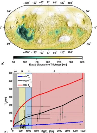
Models of thermal evolution in a 3D geometry employing a crustal thickness whose spatial variations are consistent with gravity and topography data (e.g., Neumann et al.2004) and a crustal enrichment that matches the surface abundance of heat producing elements (Taylor et al.2006; Hahn et al.2011) indicate elastic thickness values close to 300 km at the north pole and as small as 42 km in Arsia Mons (Fig.7a). Such low values suggest that a decou-pling layer in the lower crust is still present today in this region (Grott and Breuer2010; Plesa et al.2016). The low elastic thicknesses during the Noachian period can be explained if a weak crustal rheology is assumed (Grott and Breuer 2008; Breuer et al. 2016). The evolution of the elastic lithosphere thickness predicted by the 3D thermal evolution models, accounting for a weak crustal rheology and mantle plumes, is shown in Fig.7b. These mod-els show a spatial distribution of the surface heat flow, which is dominated by the crustal thickness pattern (Plesa et al.2016) and attains the smallest values in regions covered by a thin crust (e.g., Utopia, Hellas, Agyre and Isidis impact basins), while the largest values are obtained for regions covered by a thick crust (e.g., Tharsis province). A crustal thickness di-chotomy leads to higher surface heat flow values for the southern highlands compared to the northern lowlands. If instead the crustal thickness variations are reduced by assuming a vari-able crustal density, the surface heat flow shows a rather homogeneous distribution (Plesa et al.2016). The signature of mantle plumes may become visible on the surface heat flow maps if an activation volume of 10 cm3/mol is considered, which leads to a strong increase
of viscosity with pressure of about two orders of magnitude. Nevertheless, for a variety of parameters, the models predict that the location of mantle plumes is unlikely to affect the heat flow measurement. The difference between the heat flow value that will be obtained by the HP3instrument and the average surface heat flow will be less than 5 mW/m2(Plesa et al. 2016). This suggests that InSight will return a representative value for the average surface heat flow.
The average surface heat flow is an important quantity which can be directly related to the bulk abundance of HPE in the silicate part of the planet (mantle and crust) by using the so-called Urey ratio, which is defined as the ratio between the heat produced by radioactive elements in the silicate part and the heat loss over the surface. Numerical simulations show
Fig. 7 Elastic lithosphere thickness: (a) Spatial distribution of the present-day elastic lithosphere thickness
calculated using a strain rate of 10−14s−1which is characteristic for the timescale associated with the polar cap deposition at the north pole of Mars; (b) Evolution of the elastic lithosphere thickness that was computed assuming a strain rate of 10−17s−1, which is representative for convection timescales, for the entire evolution apart from the maximum value today. The latter has been calculated using the strain rate value of 10−14s−1. The colored boxes represent the elastic lithosphere thickness estimates with their corresponding error bars
that as long as the mantle of Mars is efficiently convecting, the Urey ratio converges towards a similar present-day value independent of mantle parameters such as e.g., initial mantle temperature and the distribution of heat sources between crust and mantle (Grott et al.2012; Plesa et al.2015). Thus by using the average surface heat flow, which will be derived from the InSight measurement, together with the Urey ratio, that is calculated from thermal evolu-tion models, one can estimate the bulk abundance of HPE in the interior of Mars and answer the fundamental question as to whether the amount of heat producing elements in the inte-rior of the planet is similar to previously proposed geochemical models (Wänke et al.1994; Lodders and Fegley1997; Treiman et al.1986) or lower (Phillips et al.2008).