Optimization of Network Service Chain Provisioning

HAL Id: hal-01476018

https://hal.inria.fr/hal-01476018

Submitted on 24 Feb 2017

HAL is a multi-disciplinary open access

archive for the deposit and dissemination of

sci-entific research documents, whether they are

pub-lished or not. The documents may come from

teaching and research institutions in France or

abroad, or from public or private research centers.

L’archive ouverte pluridisciplinaire HAL, est

destinée au dépôt et à la diffusion de documents

scientifiques de niveau recherche, publiés ou non,

émanant des établissements d’enseignement et de

recherche français ou étrangers, des laboratoires

publics ou privés.

Optimization of Network Service Chain Provisioning

Nicolas Huin, Brigitte Jaumard, Frédéric Giroire

To cite this version:

Nicolas Huin, Brigitte Jaumard, Frédéric Giroire. Optimization of Network Service Chain

Provision-ing. IEEE International Conference on Communications 2017, May 2017, Paris, France. �hal-01476018�

Optimization of Network Service Chain

Provisioning

Nicolas Huin

Sophia Antipolis, France

Brigitte Jaumard

Computer Science and Software Eng. Concordia University Montreal (QC) Canada Email: bjaumard@cse.concordia.ca

Fr´ed´eric Giroire

Sophia Antipolis, France

Abstract—Software-Defined Networking is a new ap-proach to the design and management of networks. It decouples the software-based control plane from the hardware-based data plane while abstracting the under-lying network infrastructure and moving the network in-telligence to a centralized software-based controller where network services are deployed. The challenge is then to efficiently provision the service chain requests, while finding the best compromise between the bandwidth requirements, the number of locations for hosting Virtual Network Functions (VNFs), and the number of chain occurrences.

We propose two ILP (Integer Linear Programming) models for routing service chain requests, one of them with a decomposition modeling. We conduct extensive numerical experiments, and show we can solve exactly the routing of service chain requests in a few minutes for networks with up to 50 nodes, and traffic requests between all pairs of nodes. We investigate the best compromise between the bandwidth requirements and the number of VNF nodes.

I. INTRODUCTION

Software-Defined Networking (SDN) is a promising technology for controlling networks with a greater flex-ibility, in the context of dynamic traffic but also in the context of the steady increase of the traffic due to applications such as video on-demand or cloud gaming. SDN not only forwards traffic, but processes it as well, throughout network functions or network services.

The Network Function Virtualization (NFV) initiative was launched in the late 2012 with the intention to address the operational challenges and high costs of managing the closed and proprietary appliances deployed throughout the communication networks [1]. By virtu-alizing and consolidating network functions tradition-ally implemented in dedicated hardware (called middle-boxes), using cloud technologies, network operators can achieve greater agility and accelerate new service de-ployments while driving down both operational (OpEx) and capital costs (CapEx) [2]. In any given network, some nodes are selected in order to be VNF node. Any virtual network function (VNF), hosted on such a node,

may then run on a single or on a set of Virtual Machines (VMs), instead of having custom hardware appliances.

Service Function Chaining (SFC) refers to an ordered sequence of service functions that a specific flow must go through. It is used by cloud providers and network operators to set up suites or catalogs of connected ser-vices that enable the use of a single network connection for many services, with different characteristics. For in-stance, cloud providers must host enterprise applications that access databases and make bulk data transfers to and from customers’ private networks constantly while communications service providers carry email, voice, video, Web traffic and downloads. Each data type bene-fits from specific types of related services. For instance, an email service chain, for example, would include virus, spam and phishing detection and could be routed through connections offering no delay and with jitter guarantees. The question is then to perform efficiently the service chaining provisioning, i.e., where to place instances of VNFs on servers in a NFV infrastructure to accommodate the traffic for a given set of SFC requests. However, operators/providers have multiple competing goals to consider when placing VNFs. On the one hand, they may want to use as few servers as possible in order to minimize operating costs and leave open servers for future needs [3], [4]. On the other hand, they may want to minimize the bandwidth requirement, as an indirect way to ensure low end-to-end network latency for their customers.

Our work considers an exact model that can be solved

optimally and that provides the minimum bandwidth SFC

provisioning for a given selection of VNF nodes, so that we can investigate the best compromise between the

bandwidth requirements and the number of VNF nodes.

To the best of our knowledge, we are the first to propose

an exact model, which scales well with the number of nodes and requests. We are able to solve within a few

The paper is organized as follows. In the next section, we discuss the related work. In Section III, we formally state the Service Function Chain Placement Problem. We then propose two original Integer Linear Programming (ILP) models to solve it in Section IV, with one ILP model using a decomposition modelling scheme. Solu-tions of both models are discussed in Section V and we investigate the best compromise between the number of VNF locations and the bandwidth requirements. Numer-ical results are presented in Section VI. Conclusions are drawn in the last section.

II. RELATED WORK

Following the NFV initiative in 2012 [1], several surveys are now available on NFV, see, e.g., [5], [6], [7] where the various NFV challenges are discussed. Multiple works proposed exact and partial mathematical formulations for the SFC provisioning problem. Several objective functions have been considered. In Martini et

al. [8] and Riggio et al. [9], the authors only solve the

placement and routing for each request independently. Savi et al. [10] propose an exact formulation in which the number of VNF nodes is minimized. Their model takes into account additional costs inherent to multi-core environment. However, they only provide results on a small network. A heuristic based on an ILP is proposed in Gupta et al. [11]. The authors only consider the k-shortest paths for every request in the network and a simplified node capacity constraint, for which only one function per node can be deployed. Mohammadkhan et

al. [12] propose an exact model along with heuristics

aiming at minimizing the maximum usage of CPU and links. The scope of the experiments is limited to the case in which the number of cores per service is limited to one. Luizelli et al. [4] provide an exact model minimizing the number of instances of functions in the network. However, they consider only a couple of tens of requests. In Bari et al. [13], the authors consider the operational expenditure (OpEx) for a daily traffic scenario as their objective function. The ILPs proposed in the works mentioned above do not scale for larger networks. To the best of our knowledge, using column generation, our work is the first to optimally solve the problem of SFC placement in a network with 50 nodes and for all-to-all demand scenarios. This model is also used as the base of the solution to the energy aware routing and placement of SFC proposed in [14].

III. SERVICEFUNCTIONCHAINPROVISIONING

PROBLEM

The SDN network is represented by a graph G = (V, L) where V represents the set of nodes and L the

G = (V, L) optical (grid) network

VVNF _{⊆ V = subset of nodes which are enabled to host}

virtual network functions

SD Set of node pairs with some demand

Dc

sd bandwidth demand from s to d for chain c

∆f # required cores per bandwidth unit for function f

CAPℓ transport capacity (bandwidth) of link ℓ

CAPv core capacity of node v

nc length (i.e., number of functions) of the chain c

fi

c the ithfunction in chain c

Table I: Notation

set of links. Each request is characterized by a source

vs, a destination vd, a chain c (i.e., a sequence of Virtual

Network Functions (VNFs)) and requires Dc

sd units of

bandwidth. Let F be the set of network virtual functions, indexed by f , with nF = |F |. Each service chain c

is defined as a sequence of Virtual Network Functions (VNFs), with some functions possibly repeated. We denote by nc the number of functions in c, i.e., the

length of the sequence. C is the set of all service chains. The number of cores required by function f in any chain is equal to ∆f per unit of bandwidth, i.e.,

D_sdc × ∆fc

i cores for request (vs, vd, c, D

c

sd) where f c i

denotes the ith function of chain c. Only a subset of nodes VVNF ⊂ V can host VNFs. Indeed, deployment of VNFs can be made on general purpose servers or standard IT platforms like high-performance switches, service, and storage, see, e.g., [5] for more details. Running a VNF requires a certain amount of resources, e.g., CPU, memory, disk, while the amount of required resources usually depends on the volume of traffic that passes through it. Consequently, each node v∈ VVNF_has a given core capacityCAPv. Similarly, each link ℓ of the

network has a transport capacity of CAPℓ. A summary

of the notations can be found in Table I.

The objective is to minimize the amount of bandwidth used in the SDN network in which all service chains are provisioned. It follows that each chain is assigned a path in which functions of c are encountered in the same order as in c, with some functions possibly located at the same node. Both core node and transport capacities must be satisfied.

A. Layered Graph

Following a similar idea as in [15], we use a layered graph GL _{that is defined as follows. The initial network} graph G is transformed into a layered graph GL _by adding max

c_∈Cnc layers to the graph (counting G as the

base layer, i.e., layer 0) and each layer is an exact copy of the original graph. For every node v∈ V , let videnote the corresponding node in the ith layer (i = 1, . . . , nc).

Every (i−1, i) layer pair is connected vertically by links

from vi−1 to vi.

Finding a path and a chain placement for a request (vs, vd) with chain c consists in finding a path from node

vson the first layer to node vdon the ncth layer. Indeed,

each layer represents the progression of the chain, e.g., being on the second layer means that the first function of the chain is already executed. The placement of the node is given by the link used to switch between layers. Both Integer Linear Programming (ILP) models pre-sented in the next section use the layered graph.

IV. OPTIMIZATIONMODELS

We first present an Integer Linear Program, called NFV ILP, in Section IV-A and then a reformulation of it within a Column Generation decomposition one, called NFV CG, in Section IV-B.

A. Model NFV ILP

This Integer Linear Program is based on the layered

graph described in Section III-A. It is written as follows.

Variables

• φsd,c,i_ℓ ∈ {0, 1}, where φsd,c,i_ℓ = 1 if (vs, vd, c, Dsdc ) is provisioned on link ℓ, 0

other-wise.

• asd,c,i

v ∈ {0, 1}, where asd,c,iv = 1 if fsdi is installed

on node v. If v̸∈ VVNF_{, a}sd,c,i v = 0.

Objective: minimization of the required bandwidth in the network min ∑ (vs,vd)∈SD ∑ c∈Csd D_sdc ∑ ℓ_∈L nc ∑ i=0 φsd,c,i_ℓ (1) Constraints

Flow constraints in order to translate the requirement of a path from source to destination going through the locations of the functions of the service chain requested by the node pair. Only the source node on the first layer and the destination node on the last layer can have a

positive outgoing and incoming flow respectively. ∑ ℓ∈ω+_(u) φsd,c,i_ℓ − ∑ ℓ∈ω−(u) φsd,c,i_ℓ + asd,c,iv − asd,c,iv −1= 0 v∈ V, (vs, vd)∈ SD, c ∈ Csd, 0 < i < nc (2) ∑ ℓ_∈ω+_(v) φsd,c,0_ℓ − ∑ ℓ_∈ω−(v) φsd,c,0_ℓ + asd,c,0_v = { 1 if v = vs 0 else (vs, vd)∈ SD, v ∈ V, c ∈ Csd (3) ∑ ℓ∈ω+_(v) φsd,c,nc ℓ − ∑ ℓ∈ω−(v) φsd,c,nc ℓ − asd,c,nc v = { −1 if v = vd 0 else (vs, vd)∈ SD, v ∈ V, c ∈ Csd (4)

Link capacity of the link in G is shared between each layer and cannot exceed CAPℓ.

∑ (vs,vd)∈SD ∑ c_∈Csd Dc_sd nc ∑ i=0 φsd,c,i_ℓ ≤CAPℓ ℓ∈ L. (5)

Node capacity. Each link (vi−1_{, v}i_{) between layer is}

represented by variable ai_{, so that the placement of a}

function is described by the usage of a cross-layer link. The capacity of a node is determined by the cross-layer link that are used to switch from one layer to the next.

∑ (vs,vd)∈SD ∑ c_∈Csd bc ∑ i=0 ∆fc iD c sda sd,c,i v ≤CAPu v∈ VVNF_{. (6)} B. Model NFV CG

As we will see in Section VI-C, the ILP presented in the previous paragraph does not scale well for medium to large networks. We thus propose a Column Generation model. It relies on the concept of configurations, where a configuration is defined by a potential provisioning for a given request. We describe below the so-called master problem, which selects the best configurations, one for each request. We discuss the solution of the master problem in Section V, in which we use a so-called pricing problem to generate a very limited set of configurations while preserving the LP and ε ILP optimality of the solution scheme.

More formally, a configuration, i.e., a Service Path for a request (vs, vd, c, Dsdc ) is composed of: (i) a network

destination, and (ii) a set of locations for the VNFs in the SFC request. Each Service Path is thus specific to a given request and its SFC.

We use the following notations in addition to those in Table I.

• p∈ Psd, a service path from s to d. A service path

is composed of a path on the network and a set of pairs (v, f ). A pair (v, f ) means that the function

f is installed on node v.

• af_vp ∈ {0, 1}, where af_vp = 1 if f is installed on node v for service path p∈ P_sdc wrt sd, c

• δp_ℓ ∈ {0, 1}, where δp_ℓ = 1 if link ℓ belongs to path

p.

Variables

• ysd,c

p ≥ 0, where ypsd,c = 1 if demand from vs to

vd for service chain c is forwarded through service

path p, 0 otherwise.

Note that each variable y_psd,c is associated to a con-figuration, i.e., a potential provisioning for request (vs, vd, c, Dsdc ). Objective min ∑ (vs,vd)∈SD ∑ c∈Csd ∑ p∈Pc sd Dc_sdLENGTH(p) ysd,c_p (7) As for Model NFV ILP, the objective is to minimize the amount of bandwidth used in the SDN network. For a path, this amount is its length, i.e., number of hops, multiplied by the bandwidth requirement of the request. The set of constraints can then be expressed as follows. Exactly one path per demand and per chain:

∑

p∈Pc sd

ysd,c_p = 1 c∈ Csd, (vs, vd)∈ SD. (8)

Link capacity: for all ℓ∈ L, ∑ (vs,vd)∈SD ∑ c_∈Csd ∑ p_∈Pc sd Dc_sdδp_ℓysd,c_p ≤CAPℓ. (9)

Node capacity: for all v∈ VVNF_, ∑ (vs,vd)∈SD ∑ c∈Csd ∑ f∈Fc ∑ p∈Pc sd ∆fDsdc a f vpy sd,c p ≤CAPv. (10) V. SOLUTIONSCHEME

Model NFV ILP can be easily solved by an ILP solver such as Cplex. Model NFV CG requires more attention as, at first look, it has an exponential number of variables. Indeed, its linear relaxation can be solved

exactly using column generation ([16]), using a limited

number of configuration, i.e., variables. Details are given below.

A. Generalities on Column Generation

The Column Generation solution scheme is a decom-position one that combines the use of the so-called Restricted Master Problem (RMP), i.e., MP with a very small subset of configurations/columns, and the so-called pricing problem, i.e., a configuration generator. Consequently, the Restricted Master Problem selects the best provisioning, one for each request, and the pricing generates improving configurations, i.e., configurations such that, if added to the current RMP, improves the value of its linear relaxation.

RMP and PP are solved alternately until the PP is un-able to generate any new improving configuration/service path, for any request. In such a case, the optimal solution of the linear relaxation of Model NFV CG has been reached, and we derived an ILP solution, using an ILP solver on the last RMP. Accuracy of the ILP solution is measured by ε = (˜zILP− z⋆LP)/z

⋆

LP, where z

⋆

LP is the optimal value of the LP relaxation, and ˜zILP denotes the value of the ILP solution.

B. Pricing Problem

The role of the Pricing Problem is to generate a valid Service Path for a given request. Once again, the formulation relies on the layer graph (GL_{) introduced} in Section III-A. Its objective is defined by the so-called reduced cost (see [16] if not familiar with linear programming concepts).

• u(j)_{represents the vector of dual variables of}

con-straints (j) in the RMP. Note that these values are given as input to the pricing problem in the column generation solution process.

Variables:

• ai_v ∈ {0, 1}, where ai_v = 1 if fic is installed on

node v.

• φi_ℓ∈ {0, 1}, where φi_ℓ= 1 if the flow forwarded on link ℓ on layer i, i.e., links in each layer in graph

GL_.

The service path generator (pricing problem) is written for each request (vs, vd, c, Dcsd).

min D_sdc ∑ ℓ∈L nc ∑ i=0 φi_ℓ− u(8)_sd+∑ ℓ∈L u(9)_ℓ D_sdc nc ∑ i=0 φi_ℓ + Dcsd ∑ v∈V u(10)v nc ∑ i=0 ∆fc iavfic (11)

Flow conservation: they correspond to flow constraints (i.e., route) from the ith function to the (i+1)th function of the service chain associated with the vs⇝ vd request

for which the pricing problem is solved (constraints

(12)), and then flow constraints from the source node to the location of the first function of the service chain (constraints (13)), and similarly from the location of the last function of the service chain to the destination node (constraints (14)). Note that ai

v= 0 for all nodes that are

not VNF capable. Observe that the next set of constraints take care of the possibility that several VNFs can be located on the same node, including on the source or destination nodes. ∑ ℓ∈ω+_(v) φi_ℓ − ∑ ℓ∈ω−(v) φi_ℓ+ ai_v− ai_v−1 = 0 v∈ V, 0 < i < nc (12) ∑ ℓ_∈ω+_(v) φ0ℓ − ∑ ℓ_∈ω−(v) φ0ℓ+ a0v= { 1 if v = vs 0 else v∈ V (13) ∑ ℓ_∈ω+_(v) φnc ℓ − ∑ ℓ_∈ω−(v) φnc ℓ − a nc v = { −1 if v = vd 0 else v∈ V (14) Link capacity. For ℓ∈ L,

Dc_sd

nc

∑

i=0

φi_ℓ≤CAPℓ. (15)

Node capacity. For v∈ VVNF_,

nc ∑ i=0 ∆fc iD c sda i v≤CAPv. (16)

VI. NUMERICALRESULTS

In this section, we report the numerical results. First, we describe the data sets we used (Section VI-A). Then, we present the performance of NFV CG in Sec-tion VI-B. Next, in SecSec-tion VI-C, we compare the performance of the two models described in Section IV. Finally, in Section VI-D, we look at the compromise between the number of VNF nodes and the bandwidth requirements.

A. Data Sets

To emulate a realistic traffic, we used the data in [17] in conjunction with the four chains presented in Table II as in [10]. Each SFC is composed of a sequence of network virtual functions and requires a specific amount of bandwidth. We use the distribution of traffic from [17] to know the number of requests of each service type. For example, a 1TB network load is composed of 699GB of Video Streaming. This amount of traffic correspond to an equivalent of _{4× 10}699−3 requests We then choose at

random the source and destination for each request and

0 20 40 60 80 100 % of demands 0 200 400 600 800 1000 1200 Time (s) NFV_CG NFV_ILP

Figure 1: Computational times of NFV ILP and NFV CG on the germany50 network.

then aggregate the resulting set of requests with respect to their source and destination nodes. Overall, we have a total of 4× n2_{demands (each type of chains for every}

node pair).

Service Chain Chained VNFs rate % traffic Web Service NAT-FW-TM-WOC-IDPS 100 kbps 18.2%

VoIP NAT-FW-TM-FW-NAT 64 kbps 11.8% Video Streaming NAT-FW-TM-VOC-IDPS 4 Mbps 69.9% Online Gaming NAT-FW-VOC-WOC-IDPS 50 kbps 0.1%

Table II: Service chain requirements [10] When choosing the set of nodes which can host VNFs, we select the nodes based on their betweenness centrality, which is the number of paths going through the node, when considering the shortest paths between all pairs of nodes. Betweenness centrality is a good indicator of the importance of a node in the network. Programs were tested on three different networks, whose characteristics are described in Table III.

B. Performance of Model NFV CG

Table IV summarizes the performance of Model NFV CG. We present results for the 3 different topolo-gies for a selected number of VNF nodes, around the half of the size of the networks. For each instance, we simulate an overall traffic of 1 Tbps.

In the last three columns, we give the optimal value of the linear relaxation (zLP

LP), the value of the ILP solution (˜zILP) and the accuracy of the ILP solution ε. In most instances, ε = 0, meaning that we obtain the optimal ILP solution For the cases where ε > 0, its value remains very small, meaning that ˜zILPis very close to the optimal ILP value.

Lastly, we observe that the number of generated columns is fairly small in order to reach very accurate ILP solutions, taking into account that we need to select one column per request, i.e., 360, 840 and 9800 columns for data instances associated with networks Internet1, Atlanta, and Germany50, respectively.

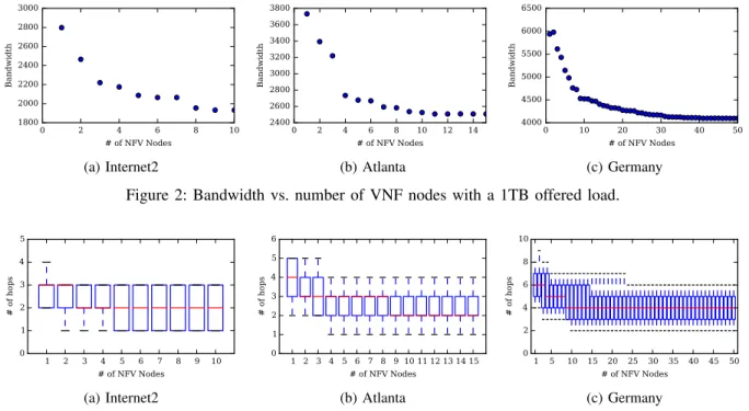
0 2 4 6 8 10 # of NFV Nodes 1800 2000 2200 2400 2600 2800 3000 Bandwidth (a) Internet2 0 2 4 6 8 10 12 14 # of NFV Nodes 2400 2600 2800 3000 3200 3400 3600 3800 Bandwidth (b) Atlanta 0 10 20 30 40 50 # of NFV Nodes 4000 4500 5000 5500 6000 6500 Bandwidth (c) Germany Figure 2: Bandwidth vs. number of VNF nodes with a 1TB offered load.

1 2 3 4 5 6 7 8 9 10 # of NFV Nodes 0 1 2 3 4 5 # of hops (a) Internet2 1 2 3 4 5 6 7 8 9 10 11 12 13 14 15 # of NFV Nodes 0 1 2 3 4 5 6 # of hops (b) Atlanta 1 5 10 15 20 25 30 35 40 45 50 # of NFV Nodes 0 2 4 6 8 10 # of hops (c) Germany

Figure 3: Distribution of the number of hops for each demand vs. number of VNF nodes with a 1TB offered load. Boxes are defined by the first and third quartiles. Ends of the whiskers correspond to the first and ninth deciles.

Network Ref. |V | |L| Internet2 [18] 10 16

Atlanta

[19] 15 44

Germany50 50 88

Table III: Network Data

# # #

Network traffic VNF generated z⋆

LP z˜ILP ε

requests nodes columns Internet2 360 5 382 2,086.7 2,086.7 0 6 382 2,064.8 2,064.4 0 7 379 2,064.4 2064.4 0 Atlanta 840 7 1,198 2,591.5 2,592.9 5.4× 10−4 8 1,611 2,581.7 2,581.7 0 9 1,266 2,534.4 2,535.8 5.6× 10−4 Germany 9,800 24 28,083 4,217.6 4,218.0 8.1× 10−5 25 28,140 4,211.9 4,212.3 8.8× 10−5 26 26,977 4,190.7 4,191.0 7.4× 10−5

Table IV: Numerical results

C. Comparison ILP vs CG

In Figure 1, we compare the two models presented in Section IV on the germany50 network. We assume all nodes are VNF enabled nodes and the number of requests varies between 10 and 100% of the requests in an all-to-all traffic scenario.

Model NFV ILP is solved exactly using the cplex ILP solver, while Model NFV CG is solved using the solution scheme described in Section V, i.e., with an ε-optimal solution scheme. As the accuracy of the

solutions of Model NFV CG is very good, the solu-tions of both models are identical. However, NFV CG takes more time as the number of requests increases. Indeed, when reaching 80% requests in the all-to-all scenario, NFV ILP does not give any solution anymore, as the cplex solver runs out of memory. Comparatively, NFV CG outputs an ε-optimal solution with all requests in less than 20 minutes. See Figure 1 for the comparison of computing times, using the ratio of the computational times.

D. Bandwidth Requirement and Delay vs. Number of VNF Capable Nodes

In this set of experiments, we want to study the impact of the number of VNF nodes on the bandwidth require-ment and the delay. Generating numerous VNF nodes could be quite costly (e.g., license price, CPU utilization, energy consumption...), and should be compensated by a significant decrease in the bandwidth requirement or justified by inacceptable delays otherwise. Our results show that this is not the case. We next discuss them in detail.

Figure 2 shows the bandwidth used for an overall 1Tbps traffic when the number of VNF nodes varies. As we allow more VNF nodes, the overall required bandwidth in the network decreases. This is as expected. Since every request requires a SFC, their provisioning

must go through VNF nodes in the required order, possibly requesting more hops than in one of the shortest paths in the network. However, what we learn from Figure 2 is that, when reaching 50% for VNF capable nodes, the bandwidth gain is getting significantly smaller. We next investigated the increase of the number of VNFs with respect to the delay, as measured by the number of hops. Results are described in Figure 3 using a box-and-whisker plot. It shows that the median value for the number of hops stabilizes as soon as the number of VNF nodes reaches 3, 9, 9 for the Internet 2, Atlanta and Germany networks, respectively. While the stabilization occurs later with bandwidth requirements, these results say that, indeed, only few requests are affected when increasing the number of VNFs beyond the 3, 9 and 9 values for Internet 2, Atlanta and Germany networks, respectively. Consequently, for homogeneous traffic as in our experiments, there is little advantage both in terms of delays and bandwidth requirements to increase much the number of VNF nodes. It might be slightly different with heterogeneous traffic, depending on the type of traffic that is impacted.

VII. CONCLUSIONS

In this paper, we look at the Service Function Chain placement problem and propose two Integer Linear Pro-gram models to solve it. We show that a simple ILP does not scale well for large networks. However, with a decomposition model like Model NFV CG, we can solve exactly the Service Function Chain Provisioning Problem. Taking into account the work of the literature, this is the first model that scales with an increasing num-ber of nodes, but also, with an increase of the numnum-ber of requests for an increase of the number of nodes pairs with service chain requirements. Model NFV CG then allowed us to look at the trade off between the network bandwidth requirement and the number of VNF capable nodes.

ACKNOWLEDGMENT

B. Jaumard has been supported by a Concordia Uni-versity Research Chair (Tier I) and by an NSERC (Natural Sciences and Engineering Research Council of Canada) grant. N. Huin and F. Giroire have been partially supported by ANR program ANR-11-LABX-0031-01 and Mitacs.

REFERENCES

[1] A. Gember, P. Prabhu, Z. Ghadiyali, and A. Akella, “Toward software-defined middlebox networking,” in ACM Workshop on

Hot Topics in Networks (HotNets), 2016, pp. 7–12.

[2] F. Callegati, W. Cerroni, C. Contoli, R. Cardone, M. Nocentini, and A. Manzalini, “SDN for dynamic NFV deployment,” IEEE

Communications Magazine, vol. 54, pp. 89 – 95, 2016.

[3] H. Moens and F. D. Turck, “VNF-P: A model for efficient placement of virtualized network functions,” in 10th International

Conference on Network and Service Management (CNSM), 2014

2014, pp. 418–423.

[4] M. Luizelli, L. Bays, L. Buriol, M. Barcellos, and L. Gaspary, “Piecing together the NFV provisioning puzzle: Efficient place-ment and chaining of virtual network functions,” in IFIP/IEEE

International Symposium on Integrated Network Management (IM), 2015, pp. 98–106.

[5] Y. Li and M. Cheng, “Software-defined network function virtual-ization: A survey,” IEEE Access, vol. 3, pp. 2542 – 2553, 2015. [6] J. Herrera and J. Botero, “Resource allocation in NFV: A com-prehensive survey,” IEEE Transactions on Network and Service

Management, vol. 13, no. 3, pp. 32–40, March 2016.

[7] R. Mijumbi, J. Serrat, J.-L. Gorricho, N. Bouten, F. D. Turck, and R. Boutaba, “Network function virtualization: State-of-the-art and research challenges,” IEEE Communications Surveys &

Tutorials, vol. 18, no. 1, pp. 236 –262, 2016.

[8] B. Martini, F. Paganelli, P. Cappanera, S. Turchi, and P. Castoldi, “Latency-aware composition of virtual functions in 5G,” in IEEE

Conference on Network Softwarization (NetSoft), 2015, pp. 1–6.

[9] R. Riggio, A. Bradai, T. Rasheed, J. Schulz-Zander, S. Kuklin-ski, and T. Ahmed, “Virtual network functions orchestration in wireless networks,” in International Conference on Network and

Service Management (CNSM), 2015, pp. 108–116.

[10] M. Savi, M. Tornatore, and G. Verticale, “Impact of processing costs on service chain placement in network functions virtualiza-tion,” in IEEE Conference on Network Function Virtualization

and Software Defined Network (NFV-SDN), Nov. 2015, pp. 191–

197.

[11] A. Gupta, M. Habib, P. Chowdhury, M. Tornatore, and B. Mukherjee, “Joint virtual network function placement and routing of traffic in operator networks,” UC Davis, Davis, CA, USA, Tech. Rep., 2015.

[12] A. Mohammadkhan, S. Ghapani, G. Liu, W. Zhang, K. Ramakr-ishnan, and T. Wood, “Virtual function placement and traffic steering in flexible and dynamic software defined networks,” in

IEEE International Workshop on Local and Metropolitan Area Networks, 2015, pp. 1–6.

[13] M. Bari, S. Chowdhury, R. Ahmed, R. Boutaba, and O. Duarte, “Orchestrating virtualized network functions,” IEEE Transactions

on Network and Service Management, vol. PP, pp. 1–1, 2016.

[14] N. Huin, B. Jaumard, and F. Giroire, “Energy-efficient service function chain provisioning,” in Proceedings of the 8th

Interna-tional Network Optimization Conference (INOC 2017), Lisbon, Portugal, 2017.

[15] A. Dwaraki and T. Wolf, “Adaptive service-chain routing for virtual network functions in software-defined networks,” in

Work-shop on Hot topics in Middleboxes and Network Function Virtu-alization (HotMIddlebox), 2016, pp. 32–37.

[16] V. Chvatal, Linear Programming. Freeman, 1983.

[17] Cisco Visual Networking Index: Forecast and Methodology,

2014–2019, CISCO, May 2015.

[18] “Internet2 network infrastructure topology,” http://www.internet2.edu/media files/422, 2014.

[19] S. Orlowski, M. Pi´oro, A. Tomaszewski, and R. Wess¨aly, “SNDlib 1.0–Survivable Network Design Library,” in

Proceed-ings of the 3rd International Network Optimization Conference (INOC 2007), Spa, Belgium, April 2007, pp. 276–286.