HAL Id: hal-02749683
https://hal.archives-ouvertes.fr/hal-02749683
Submitted on 3 Jun 2020
HAL is a multi-disciplinary open access
archive for the deposit and dissemination of
sci-entific research documents, whether they are
pub-lished or not. The documents may come from
teaching and research institutions in France or
abroad, or from public or private research centers.
L’archive ouverte pluridisciplinaire HAL, est
destinée au dépôt et à la diffusion de documents
scientifiques de niveau recherche, publiés ou non,
émanant des établissements d’enseignement et de
recherche français ou étrangers, des laboratoires
publics ou privés.
Image Time Series using Deep Learning Combined with
Graph-Based Approaches
Ekaterina Kalinicheva, Dino Ienco, Jeremie Sublime, Maria Trocan
To cite this version:
Ekaterina Kalinicheva, Dino Ienco, Jeremie Sublime, Maria Trocan. Unsupervised Change Detection
Analysis in Satellite Image Time Series using Deep Learning Combined with Graph-Based Approaches.
IEEE Journal of Selected Topics in Applied Earth Observations and Remote Sensing, IEEE, 2020, 13,
pp.1450-1466. �10.1109/JSTARS.2020.2982631�. �hal-02749683�
Unsupervised Change Detection Analysis in
Satellite Image Time Series using Deep Learning
Combined with Graph-Based Approaches
Ekaterina Kalinicheva
∗, Dino Ienco
†‡, J´er´emie Sublime
∗§and Maria Trocan
∗∗
ISEP - LISITE laboratory, DaSSIP team, 10 rue de Vanves, 92130 Issy-Les-Moulineaux, France
e-mail: [email protected]
†
INRAE - UMR TETIS, University of Montpellier, 500 rue Franc¸ois Breton, 34093 Montpellier Cedex 5, France
e-mail:[email protected]
‡
LIRMM, University of Montpellier, 161 rue Ada, 34095 Montpellier Cedex 5, France
§LIPN - CNRS UMR 7030, University Paris 13, Villetaneuse, France
e-mail:[email protected]
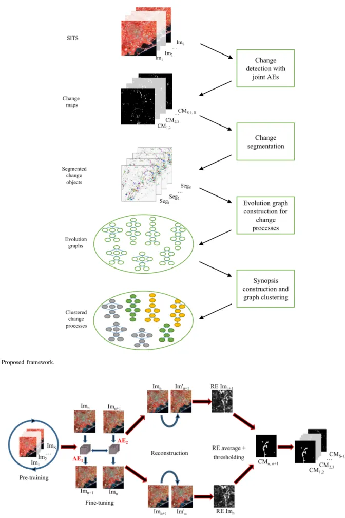
Abstract—Nowadays, huge volume of satellite images, via the different Earth Observation missions, are constantly acquired and they constitute a valuable source of information for the analysis of spatio-temporal phenomena. However, it can be challenging to obtain reference data associated to such images to deal with land use or land cover changes as often the nature of the phenomena under study is not known a priori. With the aim to deal with satellite image analysis, considering a real-world scenario where reference data cannot be available, in this paper, we present a novel end-to-end unsupervised approach for change detection and clustering for satellite image time series (SITS). In the proposed framework, we firstly create bi-temporal change masks for every couple of consecutive images using neural network autoencoders. Then, we associate the extracted changes to different spatial objects. The objects sharing the same geographical location are combined in spatio-temporal evolution graphs that are finally clustered accordingly to the type of change process with gated recurrent unit (GRU) autoencoder-based model. The proposed approach was assessed on two real-world SITS data supplying promising results.
Index Terms—satellite image time series, unsupervised learn-ing, change detection, object-oriented image analysis, pattern recognition, autoencoder, GRU, time series clustering
I. INTRODUCTION
Satellite images time series analysis algorithms have been used widely these days. Among them, there are numerous ecological applications such as the analysis and preservation of the stability of ecosystems [1], the detection and the analysis of such phenomena as deforestation and droughts [2], [3], [4], [5], real-time monitoring of natural disasters [6], [7], study of the evolution of urbanization [8], crop changes follow up [9], [10], etc. While for some applications we can create a training database with the objects presented in SITS [11], [12], for others it may be a challenging task as the nature of the researched spatio-temporal phenomena is often not known, unique or, on the contrary, has a lot of variations. For this reason, unsupervised and semi-supervised change detection and time series analysis have been a hot research topic for the past years. However, not so many successful studies are available for the proposed problematic.
Globally, we can divide the existing methods of SITS analy-sis in 1/ semi-supervised change detection which combines 1a/ anomaly detection [13], [3], [4] and 1b/ change detection in land-cover types in dense low/medium resolution time series [14], [15], and 2/ unsupervised clustering of the whole SITS [16], [17].
Most of semi-supervised SITS change detection algorithms aim to detect a particular type of change (mostly in the forest areas) based on previously available images. For example, in [13], the authors propose an algorithm for online prediction of forest fires in MODIS time series achieved by comparing real data with non-anomalous behavior modeled by Long Short-Term Memory (LSTM) network. In another study [3], the au-thors use Breaks For Additive Seasonal and Trend framework (BFAST) combined with a seasonal-trend model techniques to detect tropical forest cover loss exploiting multiple data sources (MODIS and Landsat-7). The principle of BFAST is based on iterative decomposition of time series into three components - trend, seasonal and remainder.
Similar approaches are used for change detection in land-cover types. In [14], the previously mentioned BFAST frame-work is deployed to detect land-cover changes and seasonal changes in MODIS NDVI series. To overcome this approach, in [15], the authors present a sub-annual change detection algorithm based on pixel behavior analysis. In this approach, firstly, temporal evolution of each pixel is presented as a signal with wavelet decomposition and then, each two points corre-sponding to the same acquisition day of two consecutive years are compared to determine the time of land-cover change.
To correctly model ”normal” behavior and detect seasonal trends, the SITS data should be long enough and have regular and frequent temporal resolution for the study area. At the moment, this type of freely-available time series can be pro-vided only by long existing missions such as MODIS (250 m-1 km resolution) and Landsat (30 m resolution) that are mostly used for vegetation analysis and, hence, have a low spatial resolution in favor of a high frequency of image acquisition. As the proposed techniques are adapted for low resolution
images, they are not suitable to perform SITS analysis at the local level or to distinguish different land-cover sub-classes. Moreover, the aforementioned methods are adapted for univariate data (usually, NDVI index) that sometimes can not properly characterize all the data present in SITS.
With such high resolution (HR) freely-available time se-ries as SPOT-5 and Sentinel-2, it has become possible to obtain more detailed information about the Earth surface. Unfortunately, freely-available HR SITS often contain some unexploitable images (flawed images, images with high ratio of cloud coverage, ...) or do not have sufficient temporal resolution to detect seasonal trends.
For these reasons, unsupervised HR SITS analysis demands different approaches, including ones that do not depend on temporal resolution (for example, general clustering of the whole SITS). In [18], the authors introduce a graph-based approach to detect spatio-temporal dynamics in SITS. In this method, each detected spatio-temporal phenomena is presented in a form of an evolution graph composed of spatio-temporal entities belonging to the same geographical location in mul-tiple timestamps. Following this method, [17] proposes an adapted clustering algorithm to regroup the extracted multi-annual evolution graphs in different land-cover types. This al-gorithm exploits spectral and hierarchical clustering alal-gorithms with dynamic time warping (DTW) distance measure [19] applied to the summarized representation of graph structure. It shows promising results both in intra- and inter-cite studies. In [16], the authors propose a bag of words (BoW) approach combined with Latent Dirichlet Allocation (LDA) [20] to detect different abstract clusters of land-cover. Though this algorithm is developed for synthetic aperture radar (SAR) SITS, it can be adapted for optical images after some data preprocessing. This method firstly exploits K-means clustering to determine the type of temporal evolution of each pixel with excessively large number of clusters (100-150). Secondly, every pixel is associated to a bag of words [21] representing its neighborhood patch. Each pixel of a patch contains an obtained discrete cluster value. Finally, all BoWs are regrouped in abstract classes with LDA method. Despite the fact that the proposed approaches can be used on HR images with irregular temporal resolution, they are not conceived to detect anoma-lies or land-cover changes. For example, the first method is used for clustering of the prevailing land-cover types without considering eventual land-cover changes or some anomalies. Contrary to this approach, the second method cluster the whole SITS into a large number of abstract classes without associating them to any specific spatio-temporal phenomena, so the land-cover change is not differentiated from seasonal phenological variation.
However, some applications demand another kind of SITS analysis performed at a finer level such as, for example, de-tection and classification of different types of changes applied to the urban development analysis or some local ecological disturbances.
In this paper, we propose an end-to-end unsupervised approach for the detection and classification of non-trivial changes in HR open source SITS. In our work, we imply that non-trivial changes are the changes free of seasonal trend
prevailing in SITS (trivial changes). The proposed framework firstly exploits neural network autoencoder (AE) to create bi-temporal change maps that contain only non-trivial changes (permanent changes and vegetation that do not follow the overall tendency). Afterwards, we deploy segmentation tech-niques on the extracted change areas in order to detect different spatial entities. Then we use object-based techniques to model temporal behavior of the detected change phenomena in the form of evolution graphs. Finally, we obtain a summarized representation of the extracted evolution graphs and apply Gated Recurrent Units (GRU) [22] AE combined with hi-erarchical agglomerative clustering [23] to regroup them in different types of spatio-temporal change phenomena. Our algorithm framework does not demand any training data and gives us promising results on two real-life datasets of cities of Montpellier, France and Rostov-on-Don, Russia.
Our proposed method can be used for projects studying the urban evolution of cities: changes in density of residential ar-eas, major urban structure constructions (such as transportation systems or stadiums), trends in the evolution of green areas and parks, etc. Our work is also concerned with the evolution of the landcover in crop cultures. Other applications may include ecological problematics such as the study of SITS to assess phenomena such as deforestation or the impact of droughts.
The proposed change detection approach can be applied to short time series and does not depend on the temporal resolution, as it does not demand the prior knowledge of the seasonal trend that can be computed only if the series is long enough and regularly distributed. For our knowledge, no such approaches have been proposed yet. Moreover, there is no other unsupervised framework that does both change detection and the clustering of the subsequent change graphs.
We summarize the contributions of our work as follows:
• We propose a novel framework for HR SITS change detection and clustering that do not depend on temporal resolution,
• We propose a method to model spatio-temporal change phenomena in a form of evolution graphs,
• We develop a GRU AE-based clustering model that is able to proceed varying length evolution change graphs.
II. METHODOLOGY
In this section, we present the developed framework for the detection and analysis of non-trivial changes in SITS. We start by giving the overall description of the framework and then we detail each step in the corresponding subsections.
A. Proposed framework
The proposed framework has been developed as a part of a SITS analysis algorithm. This algorithm aims to identify spatio-temporal entities presented in SITS and associate them to three different types of temporal behaviors. These temporal behaviors correspond to no change areas, seasonal changes and non-trivial changes. No change areas are mostly presented by spatio-temporal entities that have the same spectral signature over the whole SITS, such as city center, residential areas, deep water, sands, etc. Trivial (seasonal) changes correspond
to cyclic changes in vegetation prevailing in the study area. Finally, non-trivial change areas are mostly represented by permanent changes such as new constructions, changes caused by some natural disasters, crop rotations and the vegetation that do not follow the overall seasonal tendency of the study area. As non-trivial changes are less numerous and sometimes unique, they are considered by most clustering algorithms as outliers and, hence, demand a special approach for their identification and analysis that is presented in this paper. Moreover, as often we do not dispose of HR SITS with regular temporal resolution, the presented approach does not depend on temporal resolution of SITS.
The proposed approach is composed of several steps. Let RS be a time series of S co-registered images Im1, Im2, ...,
ImS acquired at timestamps T1, T2, ..., TS. The algorithm
steps are the following (Figure 1):
• We start by applying a bi-temporal non-trivial change detection algorithm [24] to every couple of consecutive images Imn-Imn+1(n ∈ [1, S − 1]) in order to get S − 1
binary change maps CM1,2, CM2,3, ..., CMS−1,S for the
whole dataset.
• We extract spatio-temporal change areas by applying the
change masks to corresponding images of SITS. Then we perform image segmentation within these change areas to obtain changed objects.
• Afterwards, the change objects located in the same ge-ographic area are grouped in temporal evolution graphs [18], [17].
• Finally, we cluster the obtained graphs using the features extracted from the change areas. We use summarized representation of graph structure - synopsis - as input sequences of clustering approach.
B. Change detection
1) Bi-temporal change detection: For the proposed frame-work, we have developed a bi-temporal non-trivial change detection algorithm [24], [25] that is applied to the whole SITS. Contrary to multi-temporal approaches that demands regular temporal resolution of SITS to get correct results, the bi-temporal approach does not assume the temporal regularity of the SITS. Moreover, when using the bi-temporal approach, we can easily detect the begin and the end of a change process in a SITS of fixed size without applying any supplementary methods. Then the obtained bi-temporal change detection results are analyzed in the context of the whole SITS.
The principle of change detection between two bi-temporal images is based on a joint AEs model that is able to reconstruct Imn+1 from Imn and vice versa by learning the translation
of image features. Areas with no changes or seasonal changes will be easily translated by the model and will have a small reconstruction error (RE). At the same time, as non-trivial changes are less numerous and some of them are unique, they will be considered as outliers and will have high reconstruction errors that can be used to map areas of non-trivial changes.
We remind the steps of our change detection algorithm [24] that are the followings, see Figure 2:
• The first step consists in model pre-training on whole SITS.
• During the second step, for each couple of images Imn
to Imn+1, we fine-tune the joint AE model by mapping
Imn to Im0n+1and Imn+1 to Im0n.
• Then, we compute the reconstruction error of Im0n+1 from Imn and vise versa for every patch of the images.
In other words, the reconstruction error of every patch is associated to the position of its central pixel on the image.
• In the last step, we detect the areas with high reconstruc-tion error using automatic Otsu’s thresholding method [26] in order to create a binary change map CMn,n+1
with the non-trivial changes.
• Finally, we obtain S − 1 CMs for whole SITS.
An AutoEncoder is a type of network where the input is the same as the output that allows us to train the model in a non-supervised manner. In this work, we use two different types of AEs convolutional AE and fullyconvolutional AE -both for change detection and further feature extraction from the change areas. The first type of AE is more complex and allows us to reduce the input 3D data in a feature vector.
In the standard convolutional AE model, during the en-coding pass, some meaningful feature maps (FM) are first extracted with convolution layers and then they are flattened and compressed in a feature vector (bottleneck of the AE) by fully-connected (FC) layers. The decoding pass is symmetrical to the encoding one and aims to reconstruct the initial patch from the feature vector. Contrary to the convolutional AE, fully-convolutional AE contains only convolution layers for both encoding and decoding steps, so the encoder output is represented only by feature maps. The models are optimized to minimize the difference between the decoded output and the initial input data. Here, for model optimization and recon-struction loss, we use the mean-squared error (MSE) (1):
M SE(o, t) = PN n=1ln N , ln= (on− tn) 2 , (1)
where o is the output patch of the model, t is the target patch and N is the number of patches per batch.
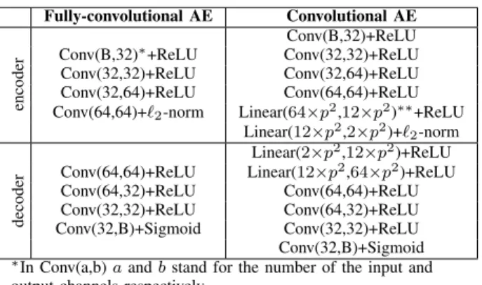
In the previous work [24], we have proposed two different AE models for bi-temporal change detection (see Table I, where p is the patch size and B is the number of spectral bands). The choice of model depends mostly on the patch size p. Note that for all convolutional layers the kernel size is 3. We equally apply batch normalization to all convolutional layers, except the one with `2-norm.
In the proposed method, the change detection is performed in a patch-wise manner for every i, j-th pixel of every couple of images (i ∈ [1, H], j ∈ [1, W ], where H and W are images height and width respectively). To pre-train the model and avoid over-fitting, we randomly select H × W/S patches from each image to form a pre-training dataset. During the pre-training phase each patch is encoded in some abstract presentation and then decoded back with a chosen AE model. We control the model loss and stop the training when the loss stabilizes.
Fig. 1. Proposed framework.
TABLE I
MODELS ARCHITECTURE FOR BI-TEMPORAL CHANGE DETECTION. Fully-convolutional AE Convolutional AE
encoder
Conv(B,32)+ReLU Conv(B,32)∗+ReLU Conv(32,32)+ReLU
Conv(32,32)+ReLU Conv(32,64)+ReLU Conv(32,64)+ReLU Conv(64,64)+ReLU Conv(64,64)+`2-norm Linear(64×p2,12×p2)∗∗+ReLU
Linear(12×p2,2×p2)+` 2-norm
decoder
Linear(2×p2,12×p2)+ReLU
Conv(64,64)+ReLU Linear(12×p2,64×p2)+ReLU
Conv(64,32)+ReLU Conv(64,64)+ReLU Conv(32,32)+ReLU Conv(64,32)+ReLU Conv(32,B)+Sigmoid Conv(32,32)+ReLU Conv(32,B)+Sigmoid
∗In Conv(a,b) a and b stand for the number of the input and
output channels respectively.
∗∗In Linear(a,b) a and b stand for the sizes of the input and
output vectors respectively.
Once the model is stable, we move on to the model fine-tuning for every couple of images Imn and Imn+1. We use
joint AEs model composed of two AEs: AE1 transforms
the patches of Imn into the patches of Im0n+1 and AE2
transforms Imn+1 into Im0n (Figure 2, Fine-tuning). Both
AEs have the same layers as the pre-trained model and are initialized with the parameters it learned. We use all image patches to fine-tune the model. The joint AEs model is trained to minimize the difference between (2):
• the decoded output of AE1 and Imn+1(loss1), • the decoded output of AE2 and Imn (loss2),
• the encoded outputs of AE1 and AE2 (feature maps for
fully-convolutional AEs and bottleneck feature vectors for convolutional AEs) (loss3).
modelLoss = loss1+ loss2+ loss3 (2)
The three losses are not weighted and equally participate in the model optimization.
We transform the patches of Imn to Im0n+1and vice versa
and calculate the reconstruction errors REn+1 and REn in
both directions and apply Otsu thresholding to the average of these errors. Otsu thresholding is calculated in a fully automatic manner to detect high RE values to produce a binary change map CMn,n+1. Finally, we obtain S − 1 bi-temporal
change maps that isolate non-trivial change areas for the whole SITS.
To estimate the quality of the model during pre-training and fine-tuning, we verify the total losses of training epochs and stop the training once the model is stable. We retain the model from the epoch that achieves the highest reconstruction capability, e.g. the smallest value in the loss function.
2) Multi-temporal change interpretation: Note that bi-temporal non-trivial changes can also be interpreted as contex-tual anomalies [27] as they depend on the overall change ten-dency presented in the couple of images. Their interpretation might be changed when passing from bi- to multi-temporal analysis as the context will be changed. To introduce multi-temporal context when detecting changes that appear between timestamps Tn and Tn+1, we propose to check if the detected
Fig. 3. Correction of detected bi-temporal contextual anomalies accordingly to multi-temporal context.
change polygon has equally appeared at certain other change maps, see Figure 3.
Firstly, we apply the aforementioned change detection al-gorithm for every couple of Imn−1-Imn+1 images (n ∈
[2, S − 1]) to calculate CMn−1,n+1. As an isolated change
area may contain several change objects, we perform image segmentation to obtain bi-temporal change polygons (the seg-mentation algorithm is explained in the following subsection and applied directly to the concatenated couples of images Imn-Imn+1and Imn−1-Imn+1). Then, we choose CMn,n+1
as reference and check if each change polygon Pch from
CMn,n+1 is equally present in CMn−1,n+1. If Pch has a
spatial intersection with any polygon(s) of CMn−1,n+1, we
mark Pch as change in the SITS context (a permanent
bi-temporal change or a part of a change process). If Pchdoes not
have spatial intersection with any polygon(s) of CMn−1,n+1,
it may belong to different types of temporal behavior:
• If Pch does not have any spatial intersection with any
polygon(s) from CMn−1,n, it is marked as false positive
(FP) change alarm caused by some image defaults and accuracy issues of unsupervised methods.
• If Pch has a spatial intersection with any polygon(s)
from CMn−1,nand with polygon(s) in at least one other
change map (CM1,2, CM2,3, CM3,4, etc), it is marked
as a part of an irregular change process.
• Finally, if Pch has intersection only with polygon(s)
from CMn−1,n and does not have any intersection with
polygons from other change maps, it is marked as a one time anomaly that happened at timestamp Tn. In this case,
all change polygons from CMn−1,nthat have intersection
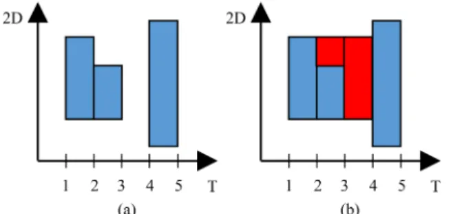
Fig. 4. Transformation of a discontinuous change process into a continuous one. Horizontal and vertical axes represent timestamps and object pixels respectively. (a)- discontinuous change process, (b)- corrected blue polygons correspond to detected change objects, red polygons are added to transform a discontinuous change process into a continuous one.
Note that here we use a threshold tint that defines the
minimum percentage of spatial intersection of Pch with other
change polygon(s), otherwise, it is considered that there is no intersection.
In this work, we suppose that every change process be-longing to the same geographical location is continuous. For example, if a pixel i, j has been classified as change in CM1,2,
CM2,3 and CM4,5, it should be also marked as change in
CM3,4 (Figure 4).
We correct the whole SITS in order to transform change processes into continuous ones. Finally, for every image Imn,
we apply the union of change maps CMn−1,nand CMn,n+1
to extract the change areas. Obviously, we apply only one change map for the first and last images of the SITS.
C. Image segmentation
In the previous section, we have proposed an approach that introduces multi-temporal context to the analysis of bi-temporal changes. As it was mentioned, an isolated change area may potentially contain several types of changes. The identification of change segments is needed at two different stages of the proposed framework. First, we detect change objects for the aforementioned algorithm. The segmentation is performed for every couple of concatenated images Imn
-Imn+1 within the associated change mask. For the second
stage, we perform the segmentation change areas of every image Imn, so the detected segments will later be used for
the construction of evolution graphs.
For both steps of the framework, we leverage a graph-based tree-merging segmentation algorithm [28] due to its ability to produce relatively large segments without merging different classes together. Large segments facilitate further construction and interpretation of evolution graphs as the shapes of some change segments may have important variations from one image to another when they are over-segmented.
The principle of the segmentation algorithm is the follow-ing: an image is represented as a graph where the pixels are nodes and resemblance values between two pixels are edges. Usually, each pixel has 8-connected neighborhood. At the beginning of the algorithm, each pixel belongs to a separate segment, then, in each step of the segmentation algorithm, the adjacent segments are merged if the difference between them
is not much less than the internal variability of these segments. To measure the resemblance value between two pixels, we use Mahalanobis distance (3):
d (~x, ~y) = q
(~x − ~y)>Cov−1(~x − ~y), (3)
where ~x, ~y are two pixels values and Cov is the covariance matrix of the image values.
The proposed algorithm requires three parameters which are σ - the standard deviation for Gaussian kernel that is used for image smoothing during the presegmentation phase, k -the constant for -the thresholding function used for segment merging, and min size that defines the minimum component size for the post-processing stage.
D. Evolution graphs
For our work, we adapt the evolution graph construction algorithm presented in [18] and [17] by passing from the anal-ysis of the whole SITS to the analanal-ysis of change areas. This approach combines graph-based techniques and data-mining technology and is used to describe a spatio-temporal evolution of a detected phenomena. The initial approach is the following: given a SITS and its associated segmentation, we choose a set of objects that corresponds to the spatial entities we want to monitor. This set of objects is called Bounding Boxes (BBs). A BB can come from any timestamp and is connected to the objects covered by its footprint at other timestamps. A BB and objects connected to it form an evolution graph. Each evolution graph can have only one BB and has to be continuous. Every object of a graph represents a node and overlapping values between two objects at two consecutive timestamps represent an edge. Objects at timestamp Tn can be connected only to
objects from Tn−1 or Tn+1, a timestamp that contains a BB
can have only one object that corresponds to this BB. 1) Bounding box selection: For BB selection, we use the same strategy as in the initial articles [18], [17], except that we do not work with the whole dataset, but only with change areas. The methodology is the following:
1) We create an empty 2D grid G that covers all changed areas. If a segment is chosen as a BB, the grid is filled with its footprint.
2) We create an empty list of candidate BB LcandBB.
3) We sort all the segments presented in SITS change areas by their size in the descending order.
4) We iterate through each segment of the sorted list. 5) We calculate the novelty and weight of each element
comparatively to already iterated segments. These values are calculated as follows:
novelty = P ix(O) − CA
P ix(O) , (4) where P ix(O) is the segments size in pixels and CA is the size of a grid area that is covered by this segment and already filled by previous candidate BBs.
weight = P ix(O) if novelty = 1 novelty if α ≤ novelty < 1 0 if novelty < α (5)
If weight ≥ α, we select this segments as a candidate BB and add it to LcandBB.
6) We iteratively update the weights in LcandBB and delete
previously detected candidate BBs if needed.
7) We iterate through the list until no more segments are left or until the grid is filled.
2) Construction of evolution graphs: In our method, we construct graphs in such a manner that every graph contains only coherent information. In other words, every BB is con-nected only to its best matching segments comparatively to neighbor BBs and each segment can belong only to one or no evolution graph.
In order to construct graphs that contain only objects belonging to the same phenomena, [18] and [17] propose to use two parameters for the construction of evolution graphs that are independent of each other: at least τ1 of the object
should be inside of BB footprint, and the intersection with the object should represent at least τ2 of BB footprint.
τ1= P ix(O) ∩ P ix(BB) P ix(BB) (6) τ2= P ix(O) ∩ P ix(BB) P ix(O) (7)
The first parameter τ1 is the most important and allows to
select only the objects that are covered the most by BB footprint. The second parameter τ2is used to keep the objects
filling only certain percentage of the footprint.
In our experiments, we are interested only in change areas of SITS, hence an isolated evolution processes may not cover the same area at different timestamps (e.g. a growing construction of a residential area).
However, it may cause that some objects will be covered by two or more BBs. To deal with this issue, we propose to associate each object only to its best matching BB, i.e the one with the highest τ1 value. In addition, for α < 0.5, an
object Oi may be a bounding box BBi of a corresponding
graph and at the same time attached to an evolution graph of a neighbor bounding box BBj. In this case, we compare
BBi’s (Oi) weight value with Oi’s τ1 value in the evolution
graph of a neighbor bounding box BBj. If τ1> weight, Oi
is attached to BBj evolution graph and the evolution graph of
BBi is destroyed and its objects are attached to other graphs,
otherwise BBi and its evolution graph are kept and Oi is
deleted from BBj’s evolution graph.
Due to pixel shift and to some false positive changes, we may observe many parasite objects presented in evolution graphs that usually correspond to crop fields. Parasite objects are the small objects attached to the beginning or to the end of the graph, these objects are the only objects presented at given timestamp and are much smaller than the footprint of the previous/next timestamp. If an evolution graph contains a parasite object, it can influence its further interpretation. Given the size of these objects, we can consider that they correspond to false positive changes and need to be deleted. To minimize the number of parasite objects, we introduce τ3
parameter that represents the minimum ratio between coverage of two consecutive timestamps.
τ3= Pq 1P ix(O n+1 i ) Pr 1P ix(Ojn) , (8)
where q and r are the number of objects at timestamps Tn+1
and Tn respectively, P ix(Oin+1) is i-th object at timestamp
Tn+1and P ix(Onj) is j-th object at timestamp Tn.
E. Graph synopsis and feature extraction
To cluster the extracted evolution change graphs, we calcu-late each graph synopsis as in [17]. A synopsis summarize the information about each graph and allow to compare them with each other. A synopsis Q is defined as a sequence of the same length as the corresponding evolution graph. Each timestamp Tnof the sequence Q contains the aggregated values of graphs
objects at this timestamp. The influence of each object at the aggregated value at the timestamp Tn is proportional to its
size and calculated as follows:
Qn = Pr 1P ix(O n j) · vj Pr 1P ix(O n j) (9)
where Qn is the synopsis value at timestamp Tn, P ix(Ojn) is
the size of a j-th object at timestamp Tn (j ∈ [1, r], where r
is the total number of the objects presented in the evolution graph E at the timestamp Tn) and vj is the corresponding
mean of the object value.
In our work, each object is characterized by the feature val-ues extracted with deep convolutional denoising autoencoder. We add a Gaussian noise to the initial patches of the dataset during the training to extract more robust features. The noise is added only to the input of the first convolutional layer. To calculate the MSE for model optimization, we use the initial patches without noise as targets. For every pixel i, j, n its features are extracted in a patch-wise manner.
The choice of feature extraction and its efficiency is de-scribed in the next section, where we compare the clustering performance for our proposed framework using a feature extraction step and also using raw pixel values for graph descriptors.
All the images are normalized using dataset mean and standard deviation before texture extraction.
In our proposed framework, the feature extraction steps are the following:
1) We extract patches of size p for every pixel of every image of SITS to train convolutional AE model. 2) We divide the extracted patch dataset in training and
validation parts (67% and 33%). Validation part is used for early stopping algorithm [29] that prevents our model from over-fitting and works in an unsupervised manner. The more the model is generalized- the more robust features we get.
3) We train the AE model in such manner that every patch from the training dataset is firstly encoded in a feature vector and then is decoded back to the initial patch. We use mean square error of the patch reconstruction to optimize the model at each iteration.
4) The early stopping algorithm is applied at every epoch and check the loss value when fitting validation dataset to the obtained model. If the validation loss does not improve during chosen number of epoch, the model is considered stable and the training is stopped.
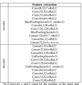
5) We use the encoding part of the AE to encode every patch of SITS change areas in a feature vector. The feature extraction model is presented in Table II, where f is the size of the encoded feature vector. Note that for all convolutional layers the kernel size is 3. We equally apply batch normalization to all convolutional layers.
TABLE II
FEATURE EXTRACTION MODEL. Feature extraction encoder Conv(B,32)∗+ReLU Conv(32,32)+ReLU Conv(32,64)+ReLU Conv(64,64)+ReLU MaxPooling(kernel=3, stride=3) Conv(64,128)+ReLU Conv(128,128)+ReLU MaxPooling(kernel=3) Linear(128,64)∗∗+ReLU Linear(64,32)+ReLU Linear(32,f)+`2-norm decoder Linear(f,32)+ReLU Linear(32,64)+ReLU Linear(64,128)+ReLU UnPooling(kernel=3) Conv(128,128)+ReLU Conv(128,64)+ReLU UnPooling(kernel=3, stride=3) Conv(64,64)+ReLU Conv(64,32)+ReLU Conv(32,32)+ReLU Conv(32,B)+ReLU
∗In Conv(a,b) a and b stand for the number of the input and
output channels respectively.
∗∗In Linear(a,b) a and b stand for the sizes of the input and
output vectors respectively.
F. Clustering
In the presented framework, we propose to use GRU [22] AE combined with hierarchical agglomerative clustering [23] to regroup the obtained evolution graphs. GRU is a recur-rent neural networks-based (RNN) type of NN that is able to process time series in order to extract some meaningful information from it. Unlike many other approaches for time series analysis, RNN is able to deal with varying sequence lengths.
In general, RNN is constructed as follows: let X = {x1, x2, ..., xn, ..., xS} be a sequence composed of S
times-tamps. In addition to the sequence values, each timestamp Tn
is associated to a hidden state hn (Figure 5) which represent
the accumulative value of the previous hidden states of the sequence. The final hidden state hS characterizes the whole
sequence and is used afterwards for classification or clustering. The main problem of RNN is that the value of each hidden state hn depends only on the value of previous hidden state
hn−1, hence, RNN networks may suffer from a long-short
memory problem caused by vanishing gradient and does not
consider long term dependencies. To solve this issue, more complex Long Short-Term Memory (LSTM) networks were introduced. Contrary to RNN, LSTM contains input, output and forget gates as well as memory cell cn at each timestamp
that makes it possible to retain meaningful information from the previous steps and, as a consequence, the value of hn
depends on all the previous hidden states of the sequence and not only on hn−1. Later, to facilitate the computation
and implementation of the LSTM model, GRU networks were developed [22] for Natural Language Processing (NLP) tasks. GRU contains only update and reset gates that allows model to train faster with less memory consuming. GRU were successfully adapted for remote sensing applications and proved to be more efficient than LSTM networks in this research area as they give better or similar results to LSTM using less training parameters and time [30], [31], [32].
Fig. 5. RNN model.
To define the nature of change process, it is necessary to consider the state of sequence at the first timestamp, regardless other timestamps values. Due to the long-short memory problem, RNN does not always keep in memory the beginning of the sequences, especially when it is long. As a result, in our work, we choose more complex GRU model for clustering basing on aforementioned studies in remote sensing. The principle of GRU AE is the same as of the convolutional one mentioned before. During the encoding pass, GRU AE extracts the accumulated hidden state of the sequence hS
at the last timestamp. The last hidden state is then self-concatenated S times [33] and passed to the decoding part that aims to reconstruct the inversed initial sequence Xinv=
{xS, ..., xn, ..., x2, x1}. As it is usually recommended to set
hidden state size large (>100), we add fully-connected layers before the GRU AE bottleneck to compress the size of hidden state to ameliorate the further clustering results. The overall GRU AE schema is presented on Figure 6. Finally, we apply hierarchical clustering to the bottleneck of GRU AE to obtain the associated change clusters.
As the input sequences have varying length, some data preparation is necessary, so the GRU is able to correctly process it. Data preparation is performed for every training batch individually, after the input GRU dataset has been created. For every batch Bi, we perform the following steps
(see Figure 7):
1) We define the maximum sequence length d of Bi.
2) We zero-pad the end of all the sequences of Bi, so they
Fig. 6. GRU AE clustering model.
3) The padded sequences are passed to the encoder, for each sequence its final hidden state hS is obtained.
4) As indicated before, we use the cloned hS as the input
of GRU layer in the decoding part, where hSis repeated
S times.
5) We apply the inverted padding mask to the cloned hS
sequence that is fed to GRU layers of the decoder. 6) The output of the decoder should resemble to the
in-verted padded input sequence.
Fig. 7. Padding of data sequences. In this example, the initial sequence x1, x2, x3has the length of 3 timestamps and the maximum sequence length
per batch is d = 5. For the simplicity of representation, we do not consider the number of features of each sequence.
While the padding of the encoder input sequence allows us to proceed batches with varying length sequences, the padding of the decoder input improves the model quality, especially, it lowers the influence of sequence lengths on the extracted encoded features.
We do not divide the sequence data into training and validation datasets as the nature of some change sequences may be unique. For these reason, we control the training loss changes between two consecutive epochs to prevent the model over-fitting. We have used MSE as the loss function.
The model configuration is presented in Table III, where f is number of features of the input sequences, hidden size is the length of the hidden state vector, d is the maximum sequence length per batch, f hidden is the size of the encoded hidden state vector.
III. DATA AND DATA PRE-PROCESSING
We test the proposed approach on two real-life publicly available time series - SPOT-5 and Sentinel-2. While the first SITS contains 12 images that are irregularly sampled over 6 years, the second one contains 17 images taken over 2 years with more regular temporal resolution.
TABLE III GRUMODEL. Sequence feature extraction
enc.
GRU(f,hidden size, dropout=0.4)∗(2 layers) Linear(hidden size,f hidden)∗∗+`2-norm
dec.
Linear(f hidden,hidden size)+ReLU Repeat hidden state d times Apply inversed padding mask GRU(hidden size,f, dropout=0.4) (2 layers)
∗In GRU(a,b dropout=) a and b stand for the number of features
of the input sequence and the size of the hidden state vector.
∗∗In Linear(a,b) a and b stand for the sizes of the input and
output vectors respectively.
A. Montpellier
SPOT-5 dataset was taken over the Montpellier area, France between 2002 and 2008 and belongs to the archive Spot World Heritage1. This particular dataset was chosen due to its high
ratio of agricultural lands and progressive construction of new areas. We have filtered out the cloudy and flawed images from all the images acquired by SPOT-5 mission over the considered geographic area and obtained 12 exploitable images with irregular temporal resolution (minimum temporal distance between two consecutive images is 2 months, maximum - 14 months, average - 6 months). Distribution of dataset images is presented in Table IV. All SPOT-5 images provide green, red, NIR and SWIR bands with 10 meters resolution. The original images are clipped to rectangular shapes of 1600×1700 pixels and transformed to UTM zone 31N: EPSG Projection. The clipped image extent corresponds respectively to the following latitude and longitude in WGS-84 system:
• bottom left corner: 43°3006.044400N , 3°47030.06600E
• top right corner: 43°39022.485600N , 3°59031.59600E B. Rostov-on-Don
Sentinel-2 dataset was taken over the city of Rostov-on-Don2 (the dataset called later Rostov), Russia between 2015
and 2018. This dataset was chosen as the city of Rostov-on-Don underwent the constructions coincided with FIFA world cup 2018 and equally because it has waste agricultural areas. We have filtered out cloudy, snow-covered and flawed images
1Available on https://theia.cnes.fr/ 2Available on https://earthexplorer.usgs.gov/
TABLE IV
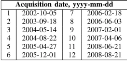
IMAGE ACQUISITION DATES FOR THEMONTPELLIER DATASET. Acquisition date, yyyy-mm-dd
1 2002-10-05 7 2006-02-18 2 2003-09-18 8 2006-06-03 3 2004-05-14 9 2007-02-01 4 2004-08-22 10 2007-04-06 5 2005-04-27 11 2008-06-21 6 2005-12-01 12 2008-08-21
from 2015 (beginning of the Sentinel-2 mission) till the end of 2018 that gave us 26 images. We deleted 6 more images from the dataset as the temporal distance between two consecutive images did not exceed 15 days. Moreover, we have deleted the first three images of the dataset because of the irregular temporal distance between them (distance between 1st and 2nd image is around one month, 2nd and 3rd - 4 months, 3rd and 4th - 5 months). Despite the fact, that our algorithm was developed for the SITS with irregular temporal resolution, it was decided to work with two datasets that differ in the terms of temporal behavior, so the Rostov dataset has ”more regular temporal resolution” comparing to the Montpellier dataset. Finally, we have obtained 17 images taken from July 2016 to November 2018 with relatively regular temporal resolution. The average gap between two consecutive images does not exceed 1.5 months, minimum - 20 days, maximum - 5 months (corresponds to winter with deleted snow-covered images). Distribution of dataset images is presented in Table V.
TABLE V
IMAGE ACQUISITION DATES FOR THEROSTOV DATASET. Acquisition date, yyyy-mm-dd
1 2016-07-15 10 2018-04-11 2 2016-08-04 11 2018-05-01 3 2016-09-13 12 2018-05-31 4 2016-11-22 13 2018-07-10 5 2017-05-01 14 2018-08-19 6 2017-06-30 15 2018-09-13 7 2017-08-09 16 2018-10-13 8 2017-09-18 17 2008-11-02 9 2018-01-11
Sentinel-2 provides multi-spectral images with different spatial resolution spectral bands. It was decided to keep only 10 meter resolution green, red and NIR bands as they contain all the essential information for general change detection and analysis. The images were provided in WGS84/UTM zone 37N projection and clipped to 2200×2400 pixels areas. The clipped image extent corresponds respectively to the following latitude and longitude in WGS-84 system:
• bottom left corner: 47°1103.566400N , 39°3403.262800E
• top right corner: 47°2407.333200N , 39°51041.32800E The pre-processing level of both datasets is 1C (orthorec-tified images, reflectance at the top of atmosphere). For this reason, both SITS were radiometrically normalized with the aim to obtain homogeneous and comparable spectral values over each dataset. For the image normalization, we have used an algorithm introduced in [34] that is based on histogram analysis of pixel distributions.
IV. EXPERIMENTS
In this section, we present parameters settings for the proposed framework and the corresponding results. We equally give some quantitative and qualitative analysis of the obtained results to show the advantages and eventual limits of the proposed approach. All the algorithms were tested on 6 cores Intel(R) Core(TM) i7-6850K CPU 3.60GHz with 32 Gb of RAM computer with a NVIDIA Titan X GPU with 12 GB of RAM and developed in Python 3 programming language using PyTorch 1.3 library on Ubuntu 16.4. tslearn library [35] was used to calculate DTW distance matrices for concurrent approaches.
Source files related to the project are available in the GitHub repository3.
A. Experimental settings
The chosen datasets have some differences in temporal resolution and images quality. For this reason, the proposed framework have some dissimilarities based on the particulari-ties of each dataset.
Due to the high temporal gap between the images of Montpellier dataset, we tend to extract the maximum of the information from it, so all extracted change sequences are kept. On the other hand, for the Rostov dataset, we keep only the change sequences that are at least 3 timestamps long. As the average temporal resolution between two images is less than two months, we consider that 2 timestamps change sequences most probably correspond to some false change alarms that could not be corrected when introducing the multi-temporal context.
For the Rostov dataset we manually apply a water mask and a mask for a part of the city with dense constructions. While the first mask is applied to eliminate FP changes caused by boats, the second one is indispensable to lower the number of FP changes caused by the shadows from tall buildings and changing luminosity that can not be corrected.
The water mask was obtained with Sen2Cor4 classification
module. Firstly, the water surfaces were detected for every image of the dataset individually. Secondly, the pixels that were marked as water for more than 50% of the images of the dataset were added to the water mask. Dense urban area mask was created manually and has almost a rectangular shape that cover a specific city area.
The last difference is related to the fact that the images of the second dataset are not perfectly aligned and some of them have one pixel size shift from the origin in different directions. This shift could not be eliminated with automatic techniques and, for this reason, we have decided to use bigger patches comparatively to Montpellier dataset for bi-temporal change detection.
1) Bi-temporal change detection: The parameters for bi-temporal change detection were set accordingly to [24]. For the Montpellier dataset, we have chosen the patch size p = 5 and the convolution AE model for feature translation as they
3Source files can be found at https://github.com/ekalinicheva/
Unsupervised-CD-in-SITS-using-DL-and-Graphs/
were proved to give the best results for 10 m resolution images [24]. Due to the shift presented in Rostov dataset, we have increased the patch size to p = 7 in order to minimize the shift influence on patch translation. We have equally chosen fully-convolutional AE model for feature translation as it gives better results than convolutional AE for bigger patch sizes [24]. The AE models for both datasets are presented in Table I. For both datasets we use only 3 bands for the change detection -red, green and NIR - as they contain the essential information about the images.
Before applying Otsu thresholding we equally exclude highv% of the highest reconstruction error values considering
they correspond to some noise and extreme outliers. The variation of the highv only balances precision/recall values,
without influencing kappa value. The higher highv is - the
higher is the recall and the smaller is the precision, and vise versa. To balance these values, we set highv to 0.5% for
both datasets. The analysis of the influence of highv value
on different metrics is detailed in the following subsection. The following quality criteria were used to evaluate the performances of the different approaches: precision (10), recall (11) and Cohen’s kappa score [36].
P recision = T rueP ositives
T rueP ositives + F alseP ositives (10)
Recall = T rueP ositives
T rueP ositives + F alseN egatives (11) To evaluate the performance of the proposed methods on two datasets, we have used ground truth maps extracted for different parts of each dataset. For the Montpellier dataset, the overall ground truth area was 600000 pixels, while for the Rostov dataset this area was 780000 pixels. The ground truth maps were manually created for the chosen areas by comparing the objects presented in the couples of images by one of the authors who is the field expert.
2) Image segmentation: To segment the extracted change areas, we have used a tree-merging bottom-up segmentation algorithm [28] described earlier. The segmentation parameters were chosen empirically and allow us to produce large seg-ments for both SITS without mixing different classes in one segment. For each dataset, we have manually chosen reference adjacent objects that have to be divided in separated segments. These objects need to have similar spectral properties, but still be easily distinguished by human eye. We set the same param-eters for single image segmentation and for the segmentation of concatenated images, so the change objects extracted from concatenated images are relevant to single-image objects.
The segmentation parameters for both datasets are the same and equal σ = 0.1, k = 7, min size = 10.
3) Multi-temporal change detection: When the prelimi-nary change maps with bi-temporal contextual anomalies are obtained, we move on to their analysis in multi-temporal context. tint should have the same value as τ1, because
both parameters define the level of spatial relation between segments at different timestamps. In other words, tint defines
if changes detected between different timestamps belong to the same change process and τ1 defines if a candidate object
belongs to a reference BB. If we set tint smaller than τ1
and a candidate change polygon is kept after multi-temporal context analysis, it may not be attached to any BB during evolution graph construction. On the contrary, if tint is set
much higher than τ1, it will produce mostly spatially compact
change processes, so small τ1 value is unnecessary.
For both datasets, we have set tint=0.4, as τ1=0.4 with
corresponding α gave the best results comparatively to other parameters combinations for both datasets (explained in the next subsection). Logically, the performance of the proposed approach fully depends on segmentation quality. The approach was qualitatively validated using manually selected reference objects.
4) Evolution graph construction: As it was mentioned before, in this work, we tend to create evolution graphs that contain only the objects that belong to the same change process. In the previous works, α value varies between 0.3 and 0.5. Smaller α values provide more overlapping graphs and, on the contrary, if α is high, we may obtain low graph coverage ratio, hence, a lot of change processes will be missed. To obtain the optimal BB coverage and graph overlapping, we choose α values 0.4 and 0.5 for the Montpellier and Rostov datasets respectively.
As every object can belong to only one evolution graph that ensures the maximum possible spatial overlay with corre-sponding BB, we propose to omit τ2value and to set τ1 value
excessively small. The smaller τ1is, the bigger graph footprint
we might obtain. However, most evolution graphs are compact independently of τ1 value. For both datasets, τ1=0.4 provided
the best graph coverage. τ3 value has to be chosen after
visual analysis of detected changes and parasite objects that correspond to false positive changes. Clearly, its value should not be too high as the footprint of change processes may have important variations at each timestamp. The parameters for evolution graph construction that gave us the best results are presented in Table VI.
TABLE VI
PARAMETERS FOR EVOLUTION GRAPHS CONSTRUCTION. Dataset α τ1 τ3
Montpellier 0.4 0.4 0.2 Rostov 0.5 0.4 0.3
5) Feature extraction autoencoder: To cluster the evolution graphs, it is necessary to extract robust descriptors of change objects. In our work, we deploy a deep convolutional AE model for non-supervised feature extraction. We use the same model for both datasets (see Table II) with patch size p=9 as it provides sufficient coverage of neighborhood pixels without high influence of objects border pixels. Contrary to the change detection algorithm, we keep all 4 spectral bands for the Montpelier dataset (Green, Red, NIR and SWIR) as SWIR band may ameliorate the clustering of some similar classes. We keep B=3 for the Rostov dataset as in change detection. We encode the patches of the Montpellier and Rostov datasets in feature vectors of size 5 and 4 respectively. Small size of feature vectors was chosen to obtain only the most representative features. Moreover, feature vectors size is equal to the number of spectral bands plus 1 (f = B + 1) to
avoid potential linear correlation between a spectral band and a corresponding element of the feature vector.
6) Evolution graph clustering: After the texture extraction, we create synopses for all evolution graphs that are then passed to the GRU AE model combined with a chosen clustering method. As we do not know beforehand the exact number of change classes presented in a SITS, we choose hierarchical agglomerative clustering algorithm.
Most of the existing clustering algorithms either demand a number of clusters as a parameter, or a set of parameters that will further define the clusters number for a given dataset. In most cases, this set of parameters is difficult to guess and varies from one dataset to another. Often the initialization of the algorithm depends on the chosen number of clusters, hence, clustering model may change drastically. At the same time, data clustering models built by the hierarchical agglom-erative algorithm do not depend on a number of clusters as at every step of the algorithm execution, it iteratively merges the two clusters with the highest likelihood value. Given these arguments, hierarchical agglomerative clustering is a good compromise between clustering quality and model complexity and makes the best choice for our generic change clustering approach.
The model parameters were set as follows for both datasets: hidden size=150, f hidden=20. Both parameters were achieved empirically, though some general recommenda-tions were followed to set the second parameter. For example, the size of AE bottleneck should correspond to the number of researched clusters [37], although, this number is not known beforehand, we can distinguish around 10-15 the most frequented types of change processes for both datasets. To improve the clustering results, the extracted sequences are normalized by their mean and standard deviation.
After the model is stabilized, we apply the hierarchical agglomerative clustering to the encoded results. As parameters for clustering algorithm, we use Ward’s linkage [23] and Euclidean distance between the encoded points. We test the results for different number of clusters in the range from 5 to 50.
Unfortunately, the right choice of the number of clusters is still an open question. No robust methods for the automatic selection of the number of clusters were find in literature and for some datasets it seems impossible to guess it. However, we can visually estimate the number of prevailing change classes and set an optimal range of the number of clusters for the hierarchical clustering. Considering the specificity of the algorithm and that its model does not depend on the selected number of clusters, we do not need to know their exact number. Furthermore, in the case of this paper, we consulted experts in cartography specialized in these areas that gave us an idea of what number of clusters and which cluster-class mapping should be expected. Our method can easily be reused in other geographic areas, with the right number of clusters found by trials and errors, or better with the help of an expert in the specific type of landscape studied.
For both datasets, we have annotated the most frequented of detected change processes to evaluate the clustering results. Note that we do not dispose of the labels for different crops,
TABLE VII
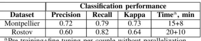
PERFORMANCE OF CHANGE DETECTION ALGORITHMS ONMONTPELLIER ANDROSTOV DATASETS IMAGES.
Classification performance Dataset Precision Recall Kappa Timea, min
Montpellier 0.72 0.79 0.73 15+8 Rostov 0.60 0.82 0.64 20+10
aPre-training+fine-tuning per couple without parallelization.
so the vegetation is annotated accordingly to its variation in the detected change sequence (for example, vegetation-weak vegetation-empty field-vegetation) and that we do not know the exact number of change process classes. For the Montpellier dataset, the annotated change processes that were regrouped in 10 classes are:
1) 5 different vegetation variations (3644, 4429, 4307, 2542 and 2206 pixels per annotated class),
2) changes in deep water (8164 pixels), 3) construction in a dense area (4122 pixels), 4) construction of a new area (13648 pixels),
5) beginning of the construction process (bare soil/construction field) (2196 pixels),
6) changes in buildings luminosity (false positive changes) (501 pixels).
For the Rostov dataset we got 11 classes:
1) 5 different vegetation variations (2864, 16930, 14805, 7521 and 6183 pixels),
2) construction of a new building (969 pixels),
3) construction of a new area (dense construction) (13669 pixels),
4) construction of a new residential area (sparse small private buildings) (241 pixels),
5) changes in bare soil (2201 pixels),
6) seasonal changes in trees/bushes growing areas (8970 pixels),
7) shadow from tall buildings (FP changes) (3708 pixels). To estimate the quality of clustering we use normalized mutual information index (NMI) [38].
B. Results
In this subsection, we present quantitative and qualitative results obtained with the proposed framework. We start by presenting the intermediate results of the framework, then we present the final results obtained by the clustering algorithm and discuss the influence of the parameters of the intermediate algorithms on the final results.
We start by bi-temporal change detection that defines the final overall accuracy of our framework. The more false positive changes there are - the more parasite objects or even parasite graphs are detected. For this reason, during the next steps, we tend to reduce their quantity by using different techniques (for example, by introducing τ3 value).
The performance of the algorithm for non-trivial bi-temporal change detection (permanent changes and vegetation that do not follow the overall tendency) is presented in Table VII. More details about the algorithms performance and its compar-ison to the state-of-art methods can be consulted in [24]. The
advantage of our method is that comparatively to the state-of-the-art algorithms, our method is less sensitive to the changing luminosity (especially in the urban area), hence, produces less false positive change alarms. It equally gives us change objects of more ”natural” shape, as we perform change detection for every pixel of the image separately by associating it to its neighborhood patch. We observe that both datasets have high recall values that indicate that most of the changes are correctly detected. At the same time, precision value is low for the Rostov dataset and depends mostly on the quality of the images itself (a lot of saturated objects and shadows are detected as changes).
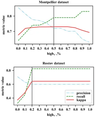
Fig. 8. The influence of highv on the recall, precision and kappa metrics
values for the Montpellier and Rostov datasets. The vertical line corresponds to the best highvfor our ground truth data.
As it was mentioned in the previous subsection, we set highv=0.5% for our method to balance the precision and recall
values. The influence of highv value on the precision, recall
and kappa values is presented on Figure 8. It was decided that the optimal threshold highv should provide the results
with recall slightly better than precision, as some FP changes will be deleted during the next steps. We observe that for the Montpellier dataset highv = 0.5% gives us the best result.
At the other hand, we notice different behavior of metrics values for the Rostov dataset ground truth and we can state less smooth changes in these values. We equally state that the best results are obtained for highv ≥ 0.2%. Therefore, it
was decided to set constant highv= 0.5% for our method to
ensure the most optimal results for both datasets.
Once the obtained change maps are analyzed in multi-temporal context, we move on to the construction of the evolu-tion graphs. Table VIII presents the evoluevolu-tion graph statistics for the chosen parameters that ensure the best coverage. It
provides total graph coverage, graph overlapping percentage, minimum graph compactness represented by the ratio of BB footprint to the total graph coverage footprint, dataset average graph compactness, percentage of graphs with compactness inferior to 50% and 75% (to justify the choice of small τ1
value).
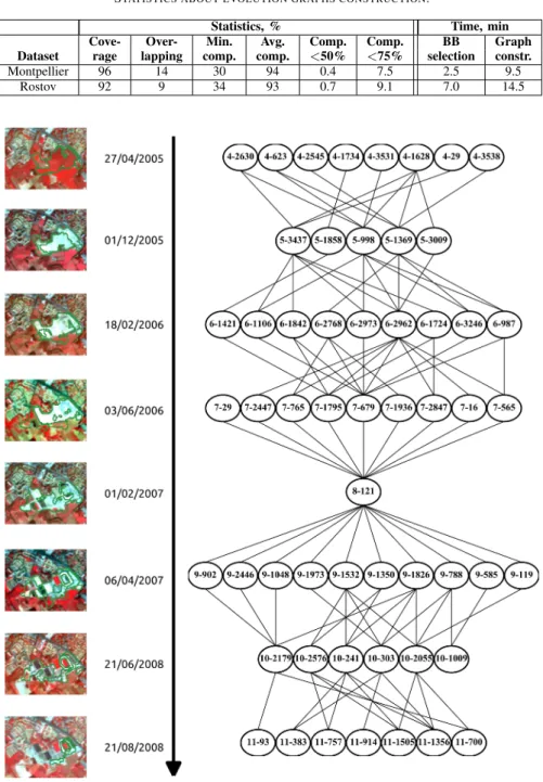
The Figure 9 presents an example of an evolution graph that corresponds to the construction of a rugby stadium. The constructed graph correctly reflects the overall change process, although, we can observe that some extracted changes and corresponding segments are not ”pure”. For example, in timestamp 18/02/2006, some small vegetation objects are attached to larger construction segments. We can also notice that the presented change process is composed of several subprocesses. One of these subprocesses starts at 03/06/2006 and at this timestamp is presented by segment 7 − 29 that corresponds to some vegetation fields that are later transformed into constructions.
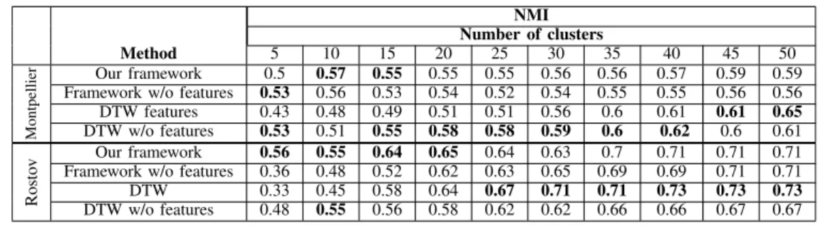
With the given evolution graph parameters, we obtain 4388 graphs for the Montpellier dataset and 1850 graphs for the Rostov dataset (after excluding 2 timestamps length sequences) that are used in totality for the AE model training. To evaluate the proposed clustering framework, we compare it with hierarchical agglomerative clustering with DTW [19] distance measure used in [17] that is equally able to process time series data with varying length. DTW is a time-series distance measure algorithm that finds optimal match between two time series by scaling one to another. Ward’s linkage was used as clustering algorithm parameter. DTW was applied to the extracted graph synopsis calculated for encoded features (called ”DTW features”) and to the raw image values (called ”DTW w/o features”). We highlight the advantage of our proposed framework by comparing it with the same framework without feature extraction (i.e. we compute the synopsis for raw image values, called ”Framework w/o features”). The obtained results are presented in Table IX for different number of clusters in order to choose the optimal one.
For both datasets we equally calculate NMI for primary change classes such as changes in vegetation, construction processes and changes in water (only for the Montpellier dataset) to verify if the extracted clusters contain only one primary type of changes (Table X).
The execution time of GRU AE combined with hierarchical agglomerative clustering and hierarchical agglomerative clus-tering with DTW distance matrix measure are presented in Table XI. Computation of DTW distance matrix is a time consuming process. hence, with growing number of change graphs, the computation time may drastically increase. At the same time, GRU AE training takes the same time for both datasets, regardless the number of graphs.
We observe that for small number of classes (10-15) our proposed framework gives the best results for the reference ground truth (10 and 11 classes for Montpellier and Rostov datatsets respectively).
However, for the Montpellier dataset, hierarchical agglom-erative clustering with DTW measure outperformed our frame-work for the number of clusters superior to 15. At the same time, primary classes of the Montpellier dataset are much
TABLE VIII
STATISTICS ABOUT EVOLUTION GRAPHS CONSTRUCTION.
Statistics, % Time, min Cove- Over- Min. Avg. Comp. Comp. BB Graph Dataset rage lapping comp. comp. <50% <75% selection constr. Montpellier 96 14 30 94 0.4 7.5 2.5 9.5
Rostov 92 9 34 93 0.7 9.1 7.0 14.5
Fig. 9. An evolution graph of rugby stadium construction.
better separated by our framework, even for small number of clusters. In general, for both datasets, NMI increases with the number of clusters, but at the same time, it may be complicated to interpret the obtained results when its number is elevated.
In our case, as the NMI is calculated at pixel and not object level, we obtain high NMI values for 11 reference classes of the Rostov dataset due to the bigger surface of vegetation changes. As DTW measure does not depend on the classes balance, it has achieved better separation of primary classes for the unbalanced dataset. Nevertheless, for large datasets, DTW computation is time-consuming, so GRU AE is the most adapted for balanced datasets of any size, and DTW approach performs better for unbalanced datasets of a small size.
After visual analysis of the obtained results and analysis of Tables IX and X, we can state that for small number of clusters our proposed framework separates the primary classes much better than the framework without feature ex-traction. It confirms that feature extraction ameliorates the class generalization for GRU, so the primary classes are better distinguished.
We observe that some construction processes that belong to the same classes for human eye are regrouped by the algorithm in different clusters. This fact justifies the ne-cessity to extract large objects during the segmentation as over-segmentation may produce numerous change graphs that correspond to the same change process, but are clustered in
TABLE IX
CLUSTERING RESULTS FOR REFERENCE CHANGE CLASSES. NMI
Number of clusters
Method 5 10 15 20 25 30 35 40 45 50
Montpellier
Our framework 0.5 0.57 0.55 0.55 0.55 0.56 0.56 0.57 0.59 0.59 Framework w/o features 0.53 0.56 0.53 0.54 0.52 0.54 0.55 0.55 0.56 0.56 DTW features 0.43 0.48 0.49 0.51 0.51 0.56 0.6 0.61 0.61 0.65 DTW w/o features 0.53 0.51 0.55 0.58 0.58 0.59 0.6 0.62 0.6 0.61
Rosto
v Our framework 0.56 0.55 0.64 0.65 0.64 0.63 0.7 0.71 0.71 0.71 Framework w/o features 0.36 0.48 0.52 0.62 0.63 0.65 0.69 0.69 0.71 0.71 DTW 0.33 0.45 0.58 0.64 0.67 0.71 0.71 0.73 0.73 0.73 DTW w/o features 0.48 0.55 0.56 0.58 0.62 0.62 0.66 0.66 0.67 0.67
TABLE X
CLUSTERING RESULTS FOR PRIMARY CLASSES. NMI Number of clusters
Method 5 10 15 20 25 30 35 40 45 50
Montpellier
Our framework 0.65 0.73 0.65 0.64 0.64 0.64 0.61 0.6 0.62 0.62 Framework w/o features 0.62 0.58 0.53 0.52 0.5 0.49 0.49 0.49 0.47 0.47 DTW 0.54 0.51 0.5 0.48 0.48 0.48 0.51 0.51 0.51 0.5 DTW w/o features 0.55 0.52 0.54 0.59 0.59 0.58 0.57 0.56 0.55 0.56
Rosto
v Our framework 0.44 0.36 0.34 0.36 0.35 0.35 0.33 0.34 0.34 0.34 Framework w/o features 0.27 0.27 0.34 0.31 0.32 0.31 0.3 0.3 0.34 0.34 DTW 0.27 0.29 0.31 0.29 0.38 0.37 0.38 0.4 0.4 0.4 DTW w/o features 0.5 0.43 0.41 0.43 0.42 0.42 0.4 0.4 0.41 0.41
different groups. However, visual examination of the results with chosen segmentation parameters shows that some graphs contain several different change sub-processes. For this reason, we may find different classes of objects at the same timestamps in one evolution graph (as in Figure 9). This class mixture may potentially influence the graph synopsis and lower the performance of our clustering algorithms.
If we lower the threshold k or increase σ values for the image segmentation, we obtain smaller segments that give us more compact evolution graphs. At the same time, the computation time for evolution graph construction will increase with the number of obtained graphs. In this case, we may obtain numerous graphs that correspond to some sub-processes that will decrease the clustering performances due to the lack of generalization of the obtained change graphs. For example, if we change only the segmentation parameters for the Montpellier dataset to σ = 0.3 and k = 6, we obtain 5316 evolution graphs that are clustered with lower precision. For example, for 15 clusters, we obtain a NMI of 0.49 and 0.5 for 10 classes and primary classes respectively contrary to 4388 graphs and 0.55 and 0.65 NMI values for the initially chosen segmentation parameters. On the other hand, if we increase the threshold k or lower σ values, we might obtain under-segmented change objects that will lead to the creation of less
TABLE XI COMPUTATION TIME.
Time, min Method Montpellier Rostov GRU AE + hier. 4 3 Hier. with DTW 16 4
”pure” evolution graphs.
The influence α, τ1 and τ3 values on the evolution graph
construction was explained in Experimental settings section. Clearly, we can attend similar effect as in previous paragraph if the number of graphs is elevated and, on the contrary, miss some change processes if the graph coverage is not sufficient.
V. CONCLUSION
In this paper, we have presented an end-to-end approach for change detection and analysis in SITS. The approach consists in the extraction of bi-temporal change maps for the whole SITS that are then analyzed in multi-temporal context in order to construct different change processes that are further regrouped in different clusters. Our framework combines graph based techniques with unsupervised feature learning with neural networks and does not depend on the temporal resolution of SITS and on its length. The proposed approach is fully unsupervised and gives us promising results on two real-life datasets. However, for unbalanced datasets, we may observe that smaller classes are not well separated from the majority ones.
Later, we are planning to work on more robust graph construction and interpretation. The graphs constructed with our method make the global description of the detected change process without considering that it may potentially contain several sub-processes. We are also looking forward to improve the algorithm for multi-temporal interpretation of detected changes by the direct integration of the filtering of parasite objects that at the moment is performed at the graph construction stage.