HAL Id: inria-00612414
https://hal.inria.fr/inria-00612414
Submitted on 10 Aug 2011
HAL is a multi-disciplinary open access
archive for the deposit and dissemination of
sci-entific research documents, whether they are
pub-lished or not. The documents may come from
teaching and research institutions in France or
abroad, or from public or private research centers.
L’archive ouverte pluridisciplinaire HAL, est
destinée au dépôt et à la diffusion de documents
scientifiques de niveau recherche, publiés ou non,
émanant des établissements d’enseignement et de
recherche français ou étrangers, des laboratoires
publics ou privés.
Domain-driven Probabilistic Analysis of Programmable
Logic Controllers
Hehua Zhang, Yu Jiang, Hung William N.N., Xiaoyu Song, Ming Gu
To cite this version:
Hehua Zhang, Yu Jiang, Hung William N.N., Xiaoyu Song, Ming Gu. Domain-driven Probabilistic
Analysis of Programmable Logic Controllers. 13th International Conference on Formal Engineering
Methods(ICFEM 2011), Oct 2011, Durham, United Kingdom. �inria-00612414�
Domain-driven Probabilistic Analysis of
Programmable Logic Controllers
Hehua Zhang1, Yu Jiang2, William N. N. Hung3, Xiaoyu Song4, and Ming Gu1
1
School of Software, TNLIST, Tsinghua University, China
2 School of Computer Science, TNLIST, Tsinghua University, China 3
Synopsys Inc., Mountain View, California, USA
4 Dept. ECE, Portland State University, Oregon, USA
Abstract. Programmable Logic Controllers are widely used in industry. Reliable PLCs are vital to many critical applications. This paper presents a novel symbolic approach for analysis of PLC systems. The main compo-nents of the approach consists of: (1) calculating the uncertainty charac-terization of the PLC systems, (2) abstracting the PLC system as a Hid-den Markov Model, (3) solving the HidHid-den Markov Model using domain knowledge, (4) integrating the solved Hidden Markov Model and the un-certainty characterization to form an integrated (regular) Markov Model, and (5) harnessing probabilistic model checking to analyze properties on the resultant Markov Model. The framework provides expected perfor-mance measures of the PLC systems by automated analytical means without expensive simulations. Case studies on an industrial automated system are performed to demonstrate the effectiveness of our approach. Keywords: PLC, Hidden Markov Model, Probabilistic Analysis
1
INTRODUCTION
Programmable Logic Controllers are widely used in industry. Many PLC appli-cations are safety critical. There are a lot of studies on the modeling and verifi-cation of PLC programs. Most of them transfer PLC programs to automata [3, 9, 1] or Petri nets [7]. Formal methods [16, 6, 14]are also proposed for analysis. Most of these methods consider the static individual PLC program that is iso-lated from its operating environment and verify some functional properties based on traversing the transferred model. The existent deterministic analysis of PLC programs are valuable, but the uncertain errors caused by noise, environment, or hardware should not be neglected [11].
In this paper, we present a symbolic framework for the formal analysis of PLC system.5 We develop a probabilistic method to model the inherent uncertainty
property of the PLC system. Then, we abstract the PLC system as a Hidden Markov Model, and generalize the Baum-Welch algorithm to solve the Hidden
5
This research is sponsored in part by NSFC Program (No.91018015, No.60811130468) and 973 Program (No.2010CB328003) of China.
Markov Model using domain knowledge of its dedicated operating environment. After that, we combine the solved Hidden Markov Model with uncertainty char-acterization of the PLC system to form an integrated Markov model. We harness probabilistic model checking to analyze properties on the regular Markov Model through PRISM [8]. Our framework also allows us to obtain some performance measures of the PLC system, such as the reliability and some other time related properties. Case studies demonstrate the effectiveness of our approaches.
2
Preliminaries
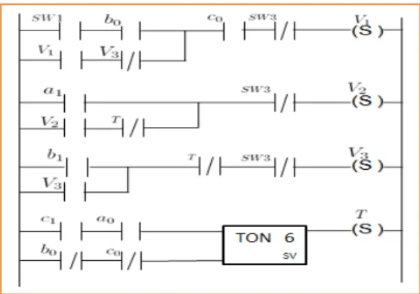
Ladder diagram (LD) is a widely used graphical programming language for PLCs. The language itself can be seen as a set of connections between logi-cal checkers (contacts) and actuators (coils). If a path can be traced between the left side of the rung and the output, through asserted contacts, the rung is true and the output coil storage bit is asserted true. If no path can be traced, then the output coil storage bit is asserted false. Fig. 1 shows a simple ladder program with some common instructions. It is made up of four ladder rungs.
The symbol −| |− is a normal open contact, representing a primary input. When the value of SW1is 1, the contact stays in the closed state, and the current
flows through the contact. The symbol −|/|− is a normal close contact. When the value of SW3is 0, the contact stays in the closed state, and the current flows
through the contact. −| | − | |− represents a serial connection of two kinds of contacts. Similarly, in the third rung, b1and V3 are connected in parallel. When
at least one value of them is 1, the current can flow through the trace. There is also a timer instruction in Fig. 1. More details can be found in [10].
Fig. 1. A simple ladder
The simplest Markov model is the Markov chain which is a random process with the property that the next state depends only on the current state. It
models the state of a system with a random variable that changes over time. A discrete time Markov model can be defined as a tupleS, π, A, L , where
• S = {S1· · · SN} is a set of states. We use qtto denote the state of the system
at time t(t ∈ N+).
• π = {π1· · · πN} is the initial state distribution, where πi = P r[q1 = Si] is
the probability that the system state at time unit 1 is Si.
• A = {aij}(∀i, j ∈ N ) is the state transition probability matrix for the system
and aij= P r[qt+1= Sj|qt= Si].
• L is a set of atomic propositions labeling states and transitions.
In a regular Markov model, the state is directly visible to the observer, and therefore the state transition probabilities are the only parameters. This model is too restrictive to be applicable to many problems of interest. Here, we extend the concept of Markov model to include the case where the observation is a probabilistic function of the state. In a Hidden Markov Model, the state is not directly visible, but the output, dependent on the state, is visible. Each state has a probability distribution over the possible output observations. Hence the sequence of observations generated by a hidden Markov model gives certain information about the sequence of states.
Formally, a Hidden Markov Model is defined as a tuple M =S, O, π, A, B, L . The items S, π, A and L are defined as above. The remaining two items of the tuple are defined as:
• O = {O1· · · OM} is a set of observations that the system can generate. We
use vtto denote the observation generated by the system at time t(t ∈ N+).
• B = {bik} is the observation state probability matrix of the system: bik =
P r[vt= Ok|qt= Si](∀Si ∈ S, ∀Ok ∈ O), which means the probability that
the system generates observation Ok in state Si.
Given an observation sequence Qo= O1O2· · · Ot, in our framework, we need
to consider the following problem:
• How to adjust the model parameters A, B to maximize P r(Qo|M ).
The problem has been solved by an iterative procedure such as the Baum-Welch method [2, 5] and equivalently the EM method [4] or gradient techniques [12]. In this paper, we generalize Baum-Welch method with additional weights.
3
SYMBOLIC FRAMEWORK
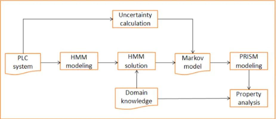
We present a symbolic framework for the formal analysis of PLC systems. The framework is applicable from the implementation process to the deployment process of the system. It contains three main procedures: (1) Uncertainty char-acterization of a PLC ladder program, which can reflect the inner quality of the system. (2) Hidden Markov Model construction and its solution, which can reflect the actual operating environment of the PLC system. (3) Reward based probabilistic model checking to analyze the performance properties of the system on the integrated Markov model. The components of the framework are shown in Fig. 2.
Fig. 2. Validation Process
3.1 Modeling Uncertainty of PLC systems
In a PLC, the program is executed through periodic scanning. In each cycle, the inputs are first sampled and read. Then, the program instructions are executed. Finally, the outputs are updated and sent to the actuators. The uncertainty characterization calculation refers to evaluating the effects of errors caused by input sampling and program execution. The sampling error happens when the actual input is 1 (or 0), but the sensor samples a 0 (or 1). Program execution error happens when the output of each ladder logic is 1 (or 0), mainly for the AN D logic (a ∧ b) and OR logic (a ∨ b), but the actual output of the logic execution turns out to be 0 (or 1). The probability of these two kinds of errors depends on noise, environment, hardware, etc.
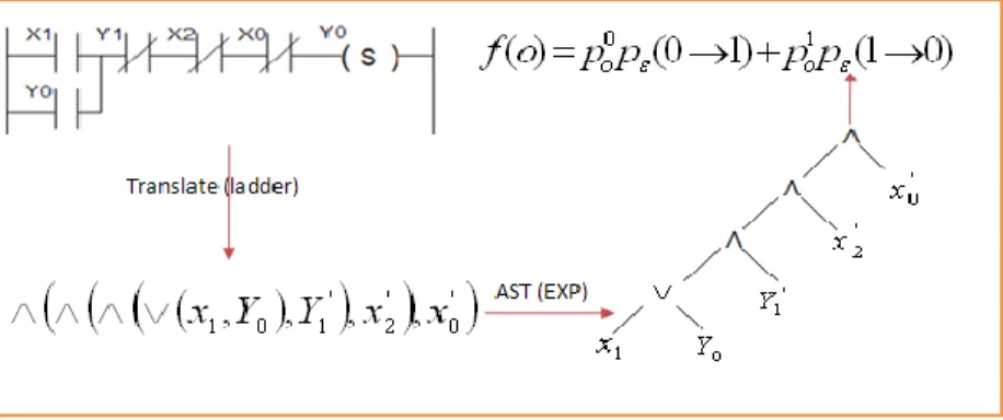
The uncertainty calculation can be divided into three steps. We first define the output of each rung on the logic checkers and the output of instructions such as timer and counter. They are connected by ladder logic (a ∧ b, a ∨ b). Then, we build an abstract syntax tree (AST) for the output expression, with which we can give a topological sort for each ladder logic (∧(a, b), ∨(a, b)). Finally, we can use the third algorithm presented in the technical report [17] to process each node in the abstract tree, until we arrive at the root node. The uncertainty characterization of this ladder rung can be described as follows:
f (o) = Po0Pε(0 → 1) + Po1Pε(1 → 0)
The first factor denotes the probability that the output of this ladder rung should be 0 (denoted by P0
o), but the root node of the abstract syntax tree propagates
a Pε(0 → 1) error. The second factor is similar. An example is shown in Fig. 3.
Because each ladder logic diagram may have many ladder rungs, we can get the following theorem:
Theorem 1. The uncertainty characterization of the whole PLC system f is
f = 1 −
i=n
Y
i=1
Where f (o)n means the uncertainty characterization of the n-th ladder rung.
Fig. 3. Uncertainty Calculation
3.2 Construction of Hidden Markov Model
Unlike the previous methods which consider an individual PLC program that is isolated from its operating environment, we construct a Hidden Markov Model (HMM) to reflect the control principle of the whole PLC system. Our model manifests the dynamic characteristics of all the possible execution paths of the PLC system. The HMM depicts how the PLC system transfers from one state to another with a hidden probability.
As mentioned in Section 2, a HMM can be defined as a tupleS, O, π, A, B, L . We abstract the PLC system as a tuple. S is the set of normal states of the PLC system. Each state of the PLC system is composed of the states of the physical devices which are actuated by the PLC ladder program. Then, each state of the PLC system can be identified by the primary outputs of the PLC ladder rungs. O contains the observations corresponding to the state set S. It is a probabilistic function of the state and can be abstracted from basic functional requirements and from events corresponding to the physical outputs of the system. L is a set of atomic propositions {L} labeling states and transitions. Since the PLC works in a periodic scanning manner and there may be timer instructions in the ladder logic diagram, we extend the label with time attribute to reflect the time property of the PLC system. The recursive syntax of the label is defined as:
L → I|T |O; I → I0|I1|0|1; T → n ∈ N+
It is composed of three components. The first component I is the sequence of the primary inputs of the PLC ladder program. The sequence will determine the outgoing transitions of each state. The second component T is the time attribute related to the timer instructions in the ladder program, which means the corresponding state Si transfers to state Sj with a time delay T . The value
of T is a positive integer N+. O is the set of observations that the primary input
will trigger in the dedicated state Sj of the transition.
3.3 Solving the Hidden Markov Model
After we obtain the knowledge about the PLC systems’ observations, states, and transitions among those states, we need to solve the unknown parameters of the HMM, especially for the parameters of the state transition probability A. We give two methods to solve the HMM by using three kinds of domain knowledge. If the domain knowledge is from a domain expert or the runtime monitoring method, the problem can be addressed by the extended Baum-Welch algorithm.
Extended Baum-Welch Method The extended Baum-Welch algorithm is based on two kinds of domain knowledge. The first kind of knowledge relies on domain expert. In a particular application, this can be done by asking the domain expert to directly provide a set of sequences of the PLC system’s obser-vations. The observation sequences are representative of the expert’s knowledge of the PLC system’s actual operating environment. The second kind of domain knowledge is from runtime monitoring. If the PLC has been deployed on the system, the system is already in use, we can observe the execution of the system many times to attain the observations.
After we get the observation sequence O(O1O2· · · OtOt+1Ot+2· · · OT) of the
HMM from time unit 1 to T , we need to adjust the model parameters M (A, B, π) to maximize the probability of the observation sequence. The Baum-Welch al-gorithm applies a dynamic programming technique to estimate the parameters. It makes use of a forward-backward procedure based on two variables:
αt(i) = P (O1O2· · · Ot, qt= Si|M ) βt(i) = P (Ot+1Ot+2· · · OT|qt= Si, M )
αt(i) is the probability of the partial observation sequence O1O2· · · Ot, and
system model is in state Si at time unit t, and βt(i) is the probability of the
partial observation sequence from t + 1 to the end, given state Si at time unit t
and the model M . We compute the parameter aij as follows:
γt(i) = P (qt= Si|O, M ) = αt(i)βt(i) N P i=1 αt(i)βt(i)
γt(i) is the probability of the system in state Siat time t, given the observation
sequence O and the model M .
ξt(i, j) = P (qt= Si, qt+1= Sj|O, M ) = αt(i)aijbj(Ot+1)βt+1(j) N P i=1 N P j=1 αt(i)aijbj(Ot+1)βt+1(j)
ξt(i, j) is the probability of the system in state Si at time t and in state Sj at
time t+1, respectively, with M and O. bj(Ot+1) denotes the probability that the
system is in state j, and the observations is Ot+1.
Then, the expected number of all the transitions from Si and the
transi-tions from Sito Sjcan be defined asPT −1t=1 γt(i) andPT −1t=1 ξt(i, j), respectively.
The expected number of observing observation Ok in state Si can be defined
as PT
t=1,vt=Okγt(i). For a single observation sequence, the iterative calculation
formulas for state transition and observation probabilities can be defined as:
aij= T −1 P t=1 ξt(i, j) T −1 P t=1 γt(i) bij = T P t=1,vt=Oj γt(i) T P t=1 γt(i)
The numerator of aijdenotes the expected number of transitions from state Sito
Sj, the denominator of aij denotes the expected number of transitions going out
of state Si. The numerator of bij denotes expected number of times in state Si
and observing symbol Oj, the denominator of bij denotes the expected number
of times in state Si.
For different observation sequences Os = [O1, O2· · · , Os], where Ok = [Ok 1,
Ok
2· · · OTk] is the kthobservation sequence, the other symbols are similar. We need
to adjust the model parameter of model M to maximize P (Os|M ). We extend the method presented in [13] with a weight Wkfor each Ok. Wkis the frequency of the
sequence Ok. We define Pk = P (Ok|M ) and P (Os|M ) =Q k
k=1PkWk. Then, the
iterative calculation formulas for state transition and observation probabilities can be changed to:
aij= k P k=1 1 PkWk T −1 P t=1 ξk t(i, j) k P k=1 1 PkWk T −1 P t=1 γk t(i) bij= k P k=1 1 PkWk T P t=1,vt=Oj γk t(i) k P k=1 1 PkWk T P t=1 γk t(i)
The meaning of the numerator and denominator of the extended formulas are the same with the original formula described above. Then, we can choose an ini-tial model M = (A, B, π) and use the iniini-tial model to compute the right side of the iterative calculation formulas. Once we get the new model M = (A, B, π), we can use M to replace M and repeat this procedure until the probability of obser-vation sequence P (Os|M ) and P (Os|M ) are equal or |P (Os|M )−P (Os|M )| < θ, θ is the precision limit you want.
With these two methods, we can build the solved HMM to show the real operating environment in an particular application. We can get value of the state transition matrix, each element aij is also identified with a label L, L → I/T /O.
3.4 Construction of Combined Regular Markov Model
The uncertainty characterization of the PLC system itself shows the inherent behaviors of the system, which evaluates the effects of the errors from input
sampling and the errors from program execution. The solved HMM shows the operating environment of the system in a particular application with the use of normal states and the transitions. Then, we construct a new Markov model to combine these two properties.
The first step is to add the abnormal state caused by the uncertainty char-acterization. Since the system would go into an abnormal state from any normal states, we build an abnormal state (U ) for all normal states (Sn). When a normal
state transits to an abnormal state, it can be recovered by the system itself or by human intervention, and reset to the initial state. We also need to add these two kinds of transitions into the solved HMM. Then, we can get all the nodes and transitions of the new Markov model M0.
The second step is to initiate the transition matrix of the new model M0. We need to assign values to different transitions. The probability of a normal state transmitting to the abnormal state depends on the value of the uncertainty calculation. The recovering transitions depends on the design of the system or the workers. After we add these states and transitions to the matrix A, the value of aij based on operating environment needs to be adjusted, by multiplying with
a coefficient. The matrix A and A0 are given by:
A = a00 a01 . . . a0n a10 a11 . . . a1n . . . ... . .. ... an0an1. . . ann A0 = a00(1 − f ) a01(1 − f ) . . . a0n(1 − f ) f a10(1 − f ) a11(1 − f ) . . . a1n(1 − f ) f . . . ... . .. ... an0(1 − f ) an2(1 − f ) . . . ann(1 − f ) f rU 0 0 . . . 0 1 − rU 0
In the new matrix, the last row and the last column are for the abnormal state U , the remaining rows and columns are for the normal states Sn. The probability
from the normal states to the abnormal state is f , which is the value of the uncertainty characterization. We know that the error probability is the same for all the normal states, because uncertainty characterization f is the inner quality of the PLC ladder program. The recovering transition probability from abnormal state U to the initial state is rU 0, The system will remain in the abnormal state
with a probability 1 − rU 0in case of some uncertainty that can-not be recovered
by the system or the operators. The transition probability between the normal states is aij(1 − f ). aij is the transition probability between the normal states
when the system is without uncertainty. The result of aij multiplied by the
coefficient 1 − f is the transition probability combined with the uncertainty characterization.
Theorem 2. The new transition matrix A0 satisfies the property of regular Markov model
Proof. According to the solved HMM’s matrix A:a00+ a01+ · · · + a0n= 1
a000+ a001+ · · · + a00n= a00(1 − f ) + a01(1 − f ) + · · · + a0n(1 − f ) + f
= a00+ a01· · · + a0n− (a00+ a01· · · + a0n)f + f
The new Markov model combines the inherent property and the operating environment of the PLC system. It closely mimics the actual execution of the PLC in real life applications. Based on this model, we can analyze the runtime properties of the PLC system using model-checking technology.
3.5 Property Analysis with PRISM
After building the integrated Markov model, we can perform probabilistic model checking using PRISM [8]. First, we need to specify the Markov model in PRISM modeling language. Second, the rewards used to specify additional quantitative measures of interest should be added into the model. Finally, we specify the properties about the PLC system.
A PRISM model comprises a set of modules which represent different as-pects of the system. The behavior of the PRISM model is specified by guarded commands. Synchronization between different modules can be implemented by augmenting guarded commands with action labels. We now describe the com-bined Markov modelS0, π0, A0, L0 in PRISM manner. The module is derived from the transition matrix A0 of the model. We declare a variable S, whose value range from [0, n+1]. Then, we build a label command for each arrow of the matrix A0 on this variable.
[Li]S = i → (a 0 i0: S 0 = 0) + (a0i1: S 0 = 1) + . . . (a0in: S 0 = n) + (f : S0 = n + 1)
Then, we focus on extending the model with rewards. There are two kinds of rewards and the structure is:
rewards ”reward name” component endrewards
The component for state rewards is guard : reward and the component for transitions is [Label] guard : reward. The guard is a predicate over the state variables, Label is the command label in each module, and the reward is a real-valued expression that will assign quantitative measures we care about the states and the transitions that are satisfied with the guard.
In the domain of PLC system, the main properties we care about are the tim-ing and the reliability of the system. So, we define two representative rewards for the model. The first is about the time property. It can be derived from the element T of the transition label L. We add a reward component [Li] true : T
for each transition into the reward. The reward reflects the elapsed time of each transition in the model. The other is a state reward. We associate a number 1 to all the normal states with the reward component S : 1. These can be used to get the long-run availability of the system. We can also define other kinds of reward, such as power consumption of each transition and state.
After we describe the probabilistic model and rewards in PRISM manner, we can analyze some properties of the model. We can specify the properties in PRISM’s specification language. We can use the P and S operator to specify quantitative time instant or long-run properties respectively. For example, we
can use the following specification to describe the execution state of the PLC system in the long-run (U denote the abnormal state of the system, S denote the normal state of the system):
Property 1: S=?[!U ], the probability that the PLC system is not in failure
in the long-run.
We can extend the above property with bounded variant of time. The following two properties specifications describe the reliability of the PLC system in a time period:
Property 2: P=?[G[0,t] !U ], the probability that the PLC system has no
error during t time units.
We can also use the R operator to get the expected value defined in terms of a reward structure. We can get many performance measures of the system. Based on the two rewards defined above, we specify two properties about time:
Property 3: R”S”=?[C≤t], the cumulative time of the system being in
normal states during the t time units.
Property 4: R”T ”=?[F U ] : the cumulative time of the system passed
before the first uncertainty state happens.
4
CASE STUDIES
We apply our framework to an actual industrial PLC system which was originally published in [15]. The system is shown in Fig. 4. It consists of three pistons (A, B, C) which are operated by solenoid valves (V1, V2, V3). Each piston has
two corresponding normally open limit sensor contacts. Three push buttons are provided to start the system (switch SW 1), to stop the system normally (switch SW 2) and to stop the system immediately in emergency (switch SW 3). In a manufacturing facility [15], such piston systems can be used to load/unload parts from a machine table, or to extend/retract a cutting tool spindle, etc.
Piston A is controlled by valve V1. When the value of V1is 1 and the piston is
at the left side, the piston will move from left to the right, and the movement is denoted by A+. When the value of V1is 0 and the piston is at the right side, the
piston will move back to the left side, and the movement is denoted by A−. We can see that the movement of A will affect the value of sensors (a0, a1). Initially,
piston A is at the left side and the normally open sensor contact a0 is closed.
Hence, the value of a0is 1, a1 is 0. When V1 turns out to be 1 at this time, the
piston will move to the right side (A+). Then, the open sensor contact a 0 will
break and the sensor contact a1 will close. Hence, the value of a0 changes to 0
and a1 changes to 1, automatically. We can use this property to design ladder
programs to control the system.
There are many PLC ladder programs that can be used to control this system. Let us see the example in Fig. 1. The ladder program is the same as the third ladder diagram in [15]. It contains four ladder rungs, which includes 8 primary
Fig. 4. Industrial automated system originally published in [15]
input contacts (SW 1, SW 3, a0, a1, b0, b1, c0, c1). SW 1 and SW 3 are changed by
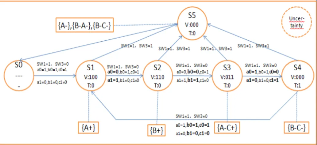
human operation, the others are automatically changed by movements of the pistons. We can construct an automata model for the operating principle of the PLC system. The state is denoted by the outputs of the ladder. The system has six normal states (S0, S1, S2, S3, S4, S5), and an uncertainty state corresponding
to the all kinds of failure caused by the uncertainty characterization. The six normal states are the states of the Hidden Markov Model. In the Fig. 5, each normal state has some corresponding observations linked by dotted line. In this system, the four states have only one corresponding observation and state S5
has 3 corresponding observations. The transitions are labeled with the primary input sequences. The time unit for each transition is 1 time unit except that the transition between state S3and S4is 6 time units. We introduce the control
theory of the model with more detail below.
At first, the system is in a blank state named S0. In this state, the pistons
stay at the left side. So, the values of (a0, a1, b0, b1, c0, c1) are (1, 0, 1, 0, 1, 0).
In the first execution cycle of the PLC system, when the worker press the start switch(SW 1), the system is activated. The values of (V1, V2, V3, T ) are (1, 0, 0, 0).
The piston A will move to the right side(A+). The values of (a
0, a1, b0, b1, c0, c1)
change to (0, 1, 1, 0, 1, 0). The second execution cycle, the values of (V1, V2, V3, T )
are (1, 1, 0, 0). The piston B will move to the right side(B+). The values of (a0, a1, b0, b1, c0, c1) changes to (0, 1, 0, 1, 1, 0). The third execution cycle, the
values of (V1, V2, V3, T ) are (0, 1, 1, 0). The piston A will move back to the left
and the piston C will move to the right side simultaneously (A−C+). The values
of (a0, a1, b0, b1, c0, c1) changes to (1, 0, 1, 0, 0, 1). If we press SW 3, the pistons B
and A will move to the left side (A−B−). The fourth execution cycle, since the value of c1and a0are 1, the timer instruction is activated. In the next five time
units, the value for output (V1, V2, V3, T ) will not change. Then, the system will
keep static for five time units. At the sixth time units, the values of (V1, V2, V3, T )
are (0, 0, 0, 1). Then, Pistons B and C will move to the left side (B−C−). The values of (a0, a1, b0, b1, c0, c1) changes to (1, 0, 1, 0, 1, 0).
Fig. 5. work theory
We can build the Hidden Markov Model for the PLC system using the oper-ating principle presented in Fig. 5. The states of the Hidden Markov Model are the normal states in the automata. The transition Label L between two hidden states is also derived from the figure. Element I is the eight primary inputs on the automata label. Element T is the time for each state transition of the original automata. The set of Observations is composed of the content in the rectangle of the Fig. 5. Hence, we can get the matrix A, B for the hidden markov model:
A = S0 S1 S2 S3 S4 S5 S0 a00a01a02a03a04a05 S1 a10a11a12a13a14a15 S2 a20a21a22a23a24a25 S3 a30a31a32a33a34a35 S4 a40a41a42a43a44a45 S5 a50a51a52a53a54a55 B = A+ B+C+A− B−C−A−B−A− S0 b00 b01 b02 b03 b04 b05 S1 b10 b11 b12 b13 b14 b15 S2 b20 b21 b22 b23 b24 b25 S3 b30 b31 b32 b33 b34 b35 S4 b40 b41 b32 b43 b44 b45 S5 b50 b51 b52 b53 b54 b55
The element a23 means the probability that the state S2 transmit to state
S3. The element b10 means the probability that we can observe that piston A
moves to the right when the system is in state S1. The semantic of the other
elements are the same.
There is a real-life application that the operating environment of the system is representative of one movement sequence O: [A+, B+, C+A−, B−C−]. Hence,
we need to solve the matrix A and B using the Baum-Welch algorithm or by simulation to get a maximum P (O|M ). Then, we need to combine the solved Hidden Markov Model M with the uncertainty state caused by the uncertainty characterization. We assume that the sampling error for each primary input contacts is 0.05, and the execution error for each ladder logic unit is 0.3. Using the method in Section 3.1, the uncertainty characterization of the PLC system is 9.80%. That means the system will go into an uncertainty state with probability
0.098 from any normal states. The system will recover to the initial state with probability 0.9 from the uncertainty state. The combined matrix is as follows:
A0 = S0 S1 S2 S3 S4 U S0 0 0.902 0 0 0 0.098 S1 0 0 0.902 0 0 0.098 S2 0 0 0 0.902 0 0.098 S3 0 0 0 0 0.902 0.098 S4 0 0.902 0 0 0 0.098 U 0.9 0 0 0 0 0.1
For a more complex example, whose operating environment is representative of three kinds of observation sequences. The observation sequences O1, O2, and
O3are [A+, A−], [A+, B+, B−A−] and [A+, B+, A−C+, B−C−], respectively. In
one thousand observations, O1 appear 200 times, O2 appear 200 times, and
O3 about 600 times. Then, we use the Baum-Welch algorithm for multiple
ob-servation sequences described in Section 3.3 and combined it with uncertainty characterization as follows: A0 = S0 S1 S2 S3 S4 S5 U S0 0 0.902 0 0 0 0 0.098 S1 0 0 0.722 0 0 0.180 0.098 S2 0 0 0 0.677 0 0.225 0.098 S3 0 0 0 0 0.902 0 0.098 S4 0 0.902 0 0 0 0 0.098 S50.902 0 0 0 0 0 0.098 U 0.9 0 0 0 0 0 0.1
We can describe the model of this example in PRISM as described in Section 3.5. We extend the model with rewards to help us analyze the system. The time property is derived from the time element T of the Markov model transition label L. In addition, we present a reward power for each state. The reward denote the power consumption for valid piston movements in each state.
At last, we can initiate some properties that we care about the system model. The first property is based on the reward oper, and denote the long term avail-ability of the system. The second property is based on the reward time, and denote the first time that it is in failure. The third property is based on the reward power, and denote the valid power consumption during 1000 time units.
– S=?[S < 6] R{”time”}=?[F S = 6] R{”power”}=?[C≤1000]
We can do more experiments on the system presented in [15]. There are four ladder programs presented in that paper. Although the four PLC programs have the same sampling error and execution error probability, their inner property are different due to different arrangements of primary inputs and logic executions. We set the input sampling error probability to 0.05 and change the value of execution error probability, denoted by ε. Using the method presented in Section 3.1, we can obtain the uncertainty characterization for the four ladder programs in Table 1.
Table 1. Uncertainty Characterization ladder ε = 0.01 ε = 0.05 ε = 0.1 ε = 0.15 ε = 0.2 ε = 0.25 ε = 0.3 ladder1 0.67% 16.87% 13.67% 12.54% 10.23% 8.69% 5.51% ladder2 0.70% 17.63% 13.89% 13.21% 11.82% 10.57% 6.62% ladder3 1.08% 28.04% 25.36% 24.57% 22.03% 21.18% 9.80% ladder4 1.15% 30.13% 26.51% 25.82% 24.65% 22.83% 10.94%
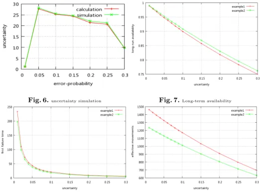
We have also devised random simulations to confirm the correctness of the uncertainty characterization. The values get by random simulations is presented in Table 2. A more visual representation for ladder3 is shown in Fig.6.
Table 2. Uncertainty Characterization By Random Simulation ladder ε = 0.01 ε = 0.05 ε = 0.1 ε = 0.15 ε = 0.2 ε = 0.25 ε = 0.3 ladder1 0.69% 17.02% 13.82% 12.66% 10.29% 8.75% 5.54% ladder2 0.74% 17.82% 14.05% 13.35% 11.91% 10.63% 6.67% ladder3 1.12% 28.22% 25.51% 24.71% 22.14% 21.27% 9.89% ladder4 1.21% 30.37% 26.68% 25.98% 24.78% 22.95% 11.16%
In the following, we will show how operating environment affect the perfor-mance of one PLC system. We use the example described in Fig. 1, which is also the same as the third ladder diagram in [15]. We have described two operating environment examples above, which are denoted by two sets of observation se-quences. We compare the three properties in these two operating environment with the help of PRISM. The results are shown in Table 3.
Table 3. Property Results
property env U=0.01 U=0.03 U=0.05 U=0.07 U=0.09 U=0.1 U=0.15 U=0.2 U=0.25 oper 1 0.989 0.968 0.947 0.928 0.909 0.900 0.857 0.818 0.783 oper 2 0.990 0.971 0.952 0.934 0.917 0.908 0.868 0.830 0.795 time 1 233 98 43 32 27 21 18 8 6 time 2 198 73 38 30 23 21 13 9 7 power 1 1462 1391 1325 1261 1200 1171 1032 908 797 power 2 1234 1181 1130 1081 1034 1011 903 804 714
From Table 3, we can see the long term availability for the second example (env=2) is always better than the first example. The first failure time for the second example come faster than the first one. The total number of valid piston movements for the first operating environment is bigger than the second. A more visual representation is shown in Fig.7,8,9 (the green line is for the second application environment). We can come to the conclusion that: for the same PLC
system, properties of the system are different in different application operating environment.
Fig. 6.uncertainty simulation Fig. 7.Long-term availability
Fig. 8.Failure-Time Fig. 9.Total-movements
5
Conclusion
This paper presents a symbolic framework for the formal analysis of PLC sys-tems. The framework is based on the uncertainty calculation of the PLC system itself and the Hidden Markov Model of the whole PLC system. We solve the Hidden Markov Model by extending the Baum-Welch algorithm or simulation to reflect the particular operating environment of the system’s application. With the help of PRISM we can perform probabilistic model checking on the combined Markov Model. The techniques used in our framework allows us to obtain ex-pected performance measures of the PLC system, which are more accurate and closer to the real-world run-time state, by automated analytical means. We can compare the performance of different PLC system designs for an particular ap-plication. Our future effort focus on the automatic techniques that transfer PLC into Hidden Markov Model and a more accurate calculation of the uncertainty characterization of PLC.
References
1. Bauer, N., Engell, S., Huuck, R., Lohmann, S., Lukoschus, B., Remelhe, M., Sturs-berg, O.: Verification of PLC Programs Given as Sequential Function Charts, Lec-ture Notes in Computer Science, vol. 3147/2004, chap. Verification, pp. 517–540. Springer Berlin / Heidelberg (2004)
2. Baum, L., Sell, G.: Growth transformations for functions on manifolds. Pacific Journal of Mathematics 27(2), 211–227 (1968)
3. Canet, G., Couffin, S., Lesage, J.J., Petit, A., Schnoebelen, P.: Towards the au-tomatic verification of PLC programs written in instruction list. In: Proc. IEEE Conf. Systems, Man and Cybernetics. pp. 2449–2454. Nashvill, TN, USA (October 2000)
4. Dempster, A., Laird, N., Rubin, D., et al.: Maximum likelihood from incomplete data via the EM algorithm. Journal of the Royal Statistical Society. Series B (Methodological) 39(1), 1–38 (1977)
5. Ephraim, Y., Dembo, A., Rabiner, L.: A minimum discrimination information ap-proach for hidden Markov modeling. IEEE Transactions on Information Theory 35(5), 1001–1013 (2002)
6. Frey, G., Litz, L.: Formal methods in PLC programming. In: Proc. IEEE Conf. Systems, Man, and Cybernetics. vol. 4, pp. 2431–2436 (October 2000)
7. Hanisch, H.M., Thieme, J., Luder, A., Wienhold, O.: Modeling of PLC behaviour by means of timed net condition/event systems. In: IEEE Int. Symp. Emerging Technologies and Factory Automation (EFTA). pp. 361–369 (1997)
8. Hinton, A., Kwiatkowska, M., Norman, G., Parker, D.: PRISM: A tool for auto-matic verification of probabilistic systems. In: Hermanns, H., Palsberg, J. (eds.) Proc. 12th International Conference on Tools and Algorithms for the Construction and Analysis of Systems (TACAS’06). LNCS, vol. 3920, pp. 441–444. Springer (2006)
9. H.X.Willems: Compact timed automata for PLC programs. Technical report csi-r9925, University of Nijmegen, Computing Science Institute (1999)
10. International Electrotechnical Commission (IEC): IEC 61131-3 Standard (PLC Programming Languages), 2.0 edn. (2003)
11. Johnson, T.L.: Improving automation software dependability: A role for formal methods? Control Engineering Practice 15(11), 1403 – 1415 (2007)
12. Levinson, S., Rabiner, L., Sondhi, M.: An introduction to the application of the theory of probabilistic functions of a Markov process to automatic speech recogni-tion. The Bell System Technical Journal 62(4), 1035–1074 (1983)
13. Rabiner, L.: A tutorial on hidden Markov models and selected applications in speech recognition. Proceedings of the IEEE 77(2), 257–286 (1989)
14. Rausch, M., Krogh, B.H.: Formal verification of PLC programs. In: Proc. American Control Conference (1998)
15. Venkatesh, K., Zhou, M., Caudill, R.J.: Comparing ladder logic diagrams and petri nets for sequence controller design through a discrete manufacturing system. IEEE Transactions on Industrial Electronics 41(6), 611–619 (December 1994)
16. Younis, M.B., Frey, G.: Formalization of existing PLC programs: A survey. In: Proc. Computational Engineering in Systems Applications (CESA) (2003) 17. Zhang, H., Jiang, Y., Hung, W.N.N., Yang, G., Gu, M.: On the uncertainty
char-acterization of programmable logic controllers (2011), http://web.cecs.pdx.edu/ ~song/research/paper_hehua_final_2.pdf
![Fig. 4. Industrial automated system originally published in [15]](https://thumb-eu.123doks.com/thumbv2/123doknet/13949019.452192/12.918.282.646.174.378/fig-industrial-automated-originally-published.webp)