Analytic moment method calculations of the drift wave spectrum

PFC/

RR-85-23 DOE/ET-51013-165

UC20G

Analytic Moment Method Calculations

of the Drift Wave Spectrum

David R. Thayer* and Kim Molvig, M.I.T.

November, 1985

Plasma Fusion Center

Massachusetts Institute of Technology Cambridge, Massachusetts 02139 USA

present address: Institute for Fusion Studies. Austin, TX

Analytic Moment Method Calculations of the I)rift Wave Spectrum

David R. Thayer and Kim Molvig,

M\.

I. T.

ABSTRACT

A derivation and approximate solution of renormalized mode coupling equations

de-scribing the turbulent drift wave spectrum is presented. Arguments are given which

in-dicate that a weak turbulence formulation of the spectrum equations fails for a system

with negative dissipation. The inadequacy of the weak turbulence theory is circumvented

by utilizing a renormalized formulation. An analytic moment method is developed to

ap-proximate the solution of the nonlinear spectrum integral equations. The solution method

employs trial functions to reduce the integral equations t algebraic equations in basic

parameters describing the spectrum. An approximate solution of the spectrum equations

is first obtained for a model dissipation with known solution, and second for an electron

dissipation in the NSA.

Analytic Moment Method Calculations of the Drift Wave Spectrum

I.

Introduction . . . .

3

II.

Derivation of Spectrum Equations: Renormalization . . . .

6

A. Spectrum Integral Equation

-

Frequency Independent Dissipation

7

1. Weak Turbulence Formulation . . . .

8

2. DIA Renormalized Formulation

. . . .

11

B. Spectrum Integral Equation

-

General Dissipation

. . . .

14

III.

Solution of Nonlinear Spectrum Integral Equations

. . . .

19

A. Spectral Trial Function

-

Frequency

. . . .

23

1. Lorentzian Line Shape

. . . .

23

2. Gaussian Line Shape . . . .

29

B. Spectral Trial Function

-

Wave Number . . . .

35

1. Moment Equation Method . . . .

36

2. Next Order Correction

. . . .

39

3. Spectrum Solution of Model Problem . . . .

43

4. Spectrum Solution of Self -

Consistent Drift Wave Problem

57

IV.

Summary and Conclusions . . . .

71

Acknowledgements

. . . .

73

Appendix A: Normalization Correction Factor in Model Problem .

74

Appendix B: Evaluation of T, Eq. (188)

. . . .

75

I. Introduction

The low frequency drift wave induced turbulence in tokamaks is thought to be one

of the dominant mechanisms driving the anomalous transport in tokamak devices. One

of the fundamental ingredients of a complete turbulence transport theory is the difficult

problem of developing a theory for the turbulence spectrum. The basic mechanism which

we consider here that allows a steady state spectrum is nonlinear mode coupling. The

negative electron drift wave dissipation drives the unstable modes, which then transfer

energy to the stable modes through nonlinear mode coupling. Physically, the lowest order

mode coupling process is a triplet interaction where two fluctuations beat together to

produce a third fluctuation. Mathematically, this process is represented as a quadratic

nonlinearity in the potential fluctuation equation.

In this article we treat two dimensional

(kr, ky)

stationary homogeneous electrostatic

drift wave turbulence which obeys a potential fluctuation equation of the form,

Here, Okw, is the frequency and wave number fourier transformed potential, and dX

E

dk'dw'dk"dw"b(k - k' - k")6(w - w' - w"). It is convenient to isolate the linear dielectric

term proportional to the frequency, w, so that the dynamical mode coupling equation for

the potential fluctuation is in general,

-i(w -

fk,)0k

dXC,;k,;kI,,f,4kw,4i,,,,,,

(2)

where -i(w

-

f2k,,)

=

wDk,/[ia/ow(wD'),

the dielectric is D =

DR + iDI,

and the

coupling coefficient is C EM/[id/w(wD,)]. For the case of density gradient driven drift

waves, with nonlinear polarization drift mode coupling dominant, the coupling coefficient

is [1),

1

e

Ck,k,kI, =

e

(k' k' - k' k")(k

- -k2)/[1

+ (kp,)

2

],

(3)

and the complex frequency, fkw, is

w-

-LDI

9k,w = Wk + ilk,w, k = 1 + 2-k, kwD(

The diamagnetic drift frequency is w* f2(p,/L.)(pky), the ion gyrofrequency is fl eB/mic, the ion inertial scale length is p, = c, /[i, and the ion sound speed is c,

(Te/mi)1/2

In Sec. II, two statistical closure schemes are analyzed in connection with the deriva-tion of the spectrum equaderiva-tions. The mode coupling equaderiva-tion for the potential fluctuaderiva-tions,

Eq. (2), is used as a starting point. Arguments are given which indicate that a weak

tur-bulence formulation of the spectrum equations fails for a system with negative dissipation, such as the drift wave problem. The failure of the weak turbulence theory is shown to be directly related to the linear instability of the triplet correlation function. The nonlinear feedback effect from higher order correlations on the evolution of the triplet correlation is obtained by formulating a renormalized theory for the spectrum, using a scheme equiva-lent to the Direct Interaction Approximation, or DIA [2]. A set of renormalized nonlinear coupled integral equations for the wave number and frequency spectrum and nonlinear complex frequency are derived.

In Sec. III, an analytic moment method is developed to approximate the solution of the nonliner spectrum integral equations. The spectrum equations are reduced to wave number space by using either a Lorentzian or a Gaussian frequency trial function, and integrating out the frequency dependence. The wave number dependent nonlinear coupled integral equations which result are expressed in terms of a wave number spectrum, a nonlinear real frequency shift, and a nonlinear frequency width. It is noted that the Lorentzian frequency function is not applicable for frequency dependent growth rates, since the wave number reduced growth rate is a frequency averaged quantity, where the spectrum is a weighting function, and most moments of a Lorentzian do not exist. The wave number spectrum problem is solved to first order by using trial functions for the wave number spectrum and frequency width. The trial functions are dependent on physically relevant parameters, the total integrated amplitude, the spectral wave number width, and the spectral frequency width. Using the trial functions in the nonlinear integral equations, and taking select wave number moments, a corresponding set of nonlinear algebraic moment equations for the parameters are determined. The parameters are obtained by solving the nonlinear coupled algebraic equations, which is done in part numerically. Equations which determine the next order correction of the parameters are presented.

The selection of the wave number moments mentioned above can be formalized using a least squares method. The nonlinear integral equations are cast into a squared functional form which is then minimized with respect to the unknown spectrum parameters. The

"best" wave number moment algebraic equations are thus obtained in a least squares sense. Preliminary calculations using the least squares moment method which give little deviation from the results presented here have been done. A complete least squares calculation of the solution for the spectrum equations will be presented in a subsequent article.

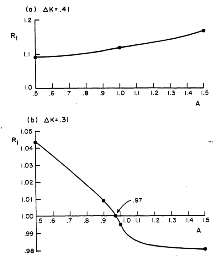
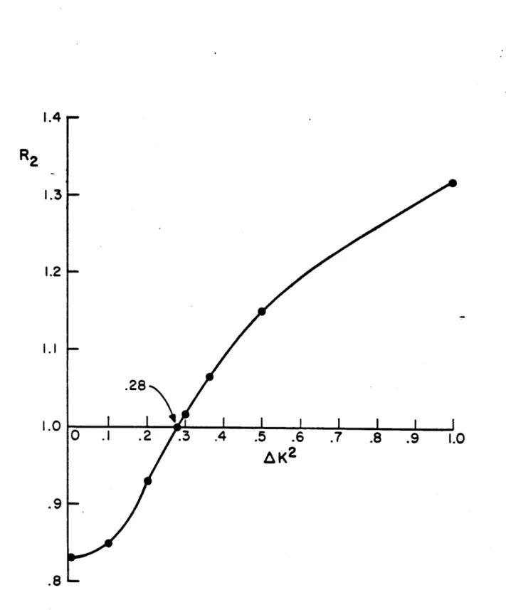
The analytic moment method is tested by approximately solving the spectrum equa-tions for a model dissipation proposed and numerically studied by Waltz [3]. This model wave number dependent growth rate exhibits damping for low and high wave numbers, with a narrow band of marginally positive growth rates between. The agreement between our approximate analytic moment method solution and the numerical solution of Waltz is excellent, both quantitatively and qualitatively. The average frequency width for this model problem is quite small, being much less than the average frequency. The analytic moment method is finally applied to the spectrum equations with a renormalized electron dissipation in the Normal Stochastic Approximation, or NSA [4]. The root mean square potential is found to be approximately, eqfm/Te ; 10', and the radial diffusion coeffi-cient is found to be approximately, D ; 1.8fli(p,/L.)p'. The results also indicate a large average spectral frequency width which is approximately equal to the average frequency. The saturation amplitude and large frequency widths are then in rough agreement with experimental observations in tokamaks. The two models indicate a large difference in fre-quency width solutions. In order to understand what causes the large frefre-quency width for the electron dissipation in the NSA, we analyze the differences in dissipation for the two models. A comparison between the model problem growth rate and the growth rate derived from the electron dissipation in the NSA is then presented, with emphasis on the resultant spectral widths. A growth rate rescaling analysis is used to verify that such a trivial adjustment in the drive cannot account for the difference in frequency width to frequency ratio for the two spectrum solutions. The spectrum solution found after rescal-ing the growth rate derived in the NSA can be used to show that the frequency width as well as the frequency itself are roughly linearly proportional to the rescalings. Conse-quently, the ratio of the frequency width to the frequency is approximately independent of the rescaling. A characteristic of the model problem growth rate is that there are few unstable triplets to drive up the noneigenmode frequency spectrum which result in a small frequency width. However, the electron dissipation in the NSA results in large spectral frequency widths, since there are many unstable triplets which drive up and populate the noneigenmode frequency spectrum.

I. Derivation of Spectrum Equations: Renormalization

A renormalized nonlinear integral equation for the turbulent spectrum is derived in

this section. The fluid-like (frequency independent) limit is taken in order to clearly demonstrate the failure of the weak turbulence formulation in a dissipative regime. The shortcoming of the weak turbulence theory is due to the associated linear instability of the triplet potential correlation function. The time asymptotic response of the linear propagator for the triplet correlation function is unbounded, when the sum of the three linear growth rates of the potential fluctuations interacting in the triplet is greater than zero. To resolve the inadequacy of the weak turbulence (linear propagator) treatment, one must include the effect of higher order correlations on the response of the triplet correlation. To this end, a renormalized theory is developed where the propagator obeys a nonlinear equation. The nonlinear feedback mechanism produces a damping which inhibits the divergence of the propagator found in the weak turbulence theory approach. This section ends with a detailed derivation of the renormalized nonlinear frequency and wa4 number spectrum integral equations for a general frequency and wave number dependent dissipation.

The usual derivation of the mode coupling equation follows from an expansion about the linear eigenfunction with a slow time separation employed [5]. The eigenmode expan-sion implies a narrow frequency spectral width of the form Sk,, : Skb(w - Wk). If the theory is extended to a noneigenmode expansion, while keeping a slow time expansion, the spectral quantity Sk,,(t) =(kw(t)4,(t)) would appear, where the frequency, W, is the Fourier transform of the fast time dependence while the explicit time dependence, t, is the slow time. Using this formulation the identification of the frequency width is difficult since a part is attributed to the explicit frequency dependence, W, and another part to the time dependence, t. Also, a slow time expansion would be suspect in a chaotic regime. Consequently, the validity of the usual mode coupling theory is doubtful for the drift wave problem in tokamaks where there is some experimental evidence suggesting that the plasma is in a highly turbulent state exhibiting a broad frequency, as well as wave number, spectrum

[6].

A. Spectrum Integral Equation - Frequency Independent Dissipation

The majority of research on the drift wave spectrum problem has dealt with a

fluid-like version of the mode coupling equation where the growth rate, Ykw, is independent of frequency, w. In these treatments the linear frequency, wk, is derived from the fluid equations while the growth rate, -yk, is usually modeled after the electron-ion dissipation found from a complete plasma kinetic theory derivation. In order to make contact with this fluid-like treatment of the spectrum problem in this section, the limit of the general mode coupling equation, Eq. (2), to frequency independent parameters, ,w -* fGi and

Ck,w;k,,w,;kI,,,W, - Ck,k,,k,,, is used to characterize the fluid limit. This limit produces a

mode coupling equation formally equivalent to the mode coupling equation derived by a fluid mechanics approach. In the following section, Sec. B, the spectrum integral equation is derived with the complete plasma kinetic theory mode coupling equation, where the complex frequency, lk,,, is a general function of wave number and frequency.

The fluid limit of the mode coupling equation in the wave number, k, time, t, domaig is

+ iQk) O (t) = dXCk,kI,k11k'(t)Okk, (t). (5) For a homogeneous system the wave number selection rule is,

(4k (t)'k,(t')) =

6(k

- k')Sk(t, t'), (6)

so that,

(qg (t)4 j (t')) = Sk(t, t'),

where, < >, is an ensemble average and the infinite normalization is deleted for simplicity

of presentation. Multiplying Eq. (5) by Oj(t') and using Eq. (6) results in the equation for the wave number spectral two time correlation function, Sk(t, t'),

( t+

I

'k Sk (t, t') = fdXCk,k',,, (A' (t')Ok, (t)Ok,, (t)),

(7)

while the equation for the one time or energy wave number spectrum, Sk(t,t), is

In order to obtain a completely closed equation for the spectrum, a relation for the triplet correlation function, (0*04), in terms of the spectrum must be obtained. Two closure schemes will be discussed. First, the closure scheme will be achieved using a weak turbulence theory [71 which employs the random phase approximation, or RPA [8]. The weak turbulence theory is then shown to be inadequate for systems with negative dissipation since the triplet correlation is linearly unstable in this theory, so that the time asymptotic limit of the triplet propagator is infinite. The need for renormalization is then motivated, so that higher order correlations can nonlinearly feedback on the response of the triplet correlation. The feature of the renormalized equations for the spectrum, which eliminates the linear instability associated with the weak turbulence theory, is the inclusion of nonlinear damping in the propagator of potential fluctuations. Second, closure will be derived using the Direct Interaction Approximation, or DIA [2]. A resolution of the problem found with weak turbulence theory is achieved since the final equations are a set of fully nonlinear coupled equations for the spectrum as well as the propagator. The DIA renormalization of the fluid-like mode coupling equation is derived in order to demonstraOI its equivalence with the renormalization scheme used in Sec. B on the complete plasma kinetic theory mode coupling equation taken in the fluid limit.

1. Weak Turbulence Formulation

Using the potential fluctuation equation, Eq. (5), an equation for the triplet,

(ki(t)4k,(t)kk,,(t)), is found by differentiation and averaging,

at

I(9kj - fl '- lfkD)] ( N ov~kk (t k"())

J

dkidk

2

[6(k

-

k

I

-

k2)Ck,k,,1 2(0j, (t)O

;(t)Ok(t)Ok,(t))

+ 6(k' -

k

1 - k2)Ck',ki,k2 ((t)4Ok (t)4kg (t)k" (t))

+

6(k"

-

k

1 - k2)Ck",,k ,k2

(4

(t) 00k(t)4k (t)4 (t)) . (9)

In a highly turbulent (random) state the ensemble average potential fluctuation is zero,

(0) = 0, and the quartic correlation can be exactly expressed as a sum of all possible

products of paired correlations plus an irreducible correlation, Q,

In this cumulant expansion it is postulated that the irreducible correlation,

Q,

is much

smaller than the product of paired correlations,

Q/

(44) (0)

< 1. The leading order

quar-tic expansion is obtained by setting the irreducible correlation to zero,

Q --

+

0. This can be

motivated by considering the relevant stochastic regime, where it is physically reasonable

to treat the potential fluctuations as normally distributed. In fact, this is equivalent to

the RPA where only the lowest order (paired) terms in the cumulant expansion are kept,

while dropping the irreducible correlation,

Q.

After using the wave number selection rule, Eq. (6), and the RPA for the cumulant

expansion of the quartic in Eq. (9), the equation for the triplet correlation is

[at-

i(llk - n - 2ku)]I (k(t)Ok'(t)Ok:'(t))

= 2[Ck,k',,, Ski (t, t)SkI, (t, t) + CkI,_k,,kSk(t,t)Sk,,(t, t)

+ Ck",-k,k Sk(t, t)Sk' (t,t)], (11)

where the symmetry

Ck,,Ik,,k = Ck,,k,,k,

and reality condition C

=

C* have been used.

The triplet equation can be solved formally in terms of a triplet propagator or Green's

function, GT(t, t'), as follows,

- iDi-

O,

- O,, G(t, t') = b(t -t'),

(12)

so that

G T(t tt exp[i49j - flk' - flk'I)( - t%), t > t' 13

Gi'(t,

t') =_ i,( '] (13)

and the solution is

(4j(t)qg,

(t)/,k ,

(t))

= ((0) Ok',(0)4k,,

(0))G

T(t,

0)

+

dt'G

T(t, t')2[Ck,k',k, Ski (t', t')Sks, (t', t')

+ Ck',-k",kSk(t', t')Sk, (t', t')

If the triplet propagator is well behaved in the time asymptotic limit, limt.x 0 Gk(t, 0) = 0,

then the initial triplet correlation will not contribute so that the final equation for the spectrum, Sk (t, t), is obtained by substituting Eq. (14) in Eq. (8),

- 2yk Sk (tt) =

JdX

dt'Gijft,t')

+

-- 2Ck,k',k" Ck',k",k Sk (t', t')Sk" (t', t')

where the symmetry Ck,,-k," = -Ck',k,,k was used.

The steady state spectrum, Sk, is obtained from Eq. (15) by taking the time asymp-totic limit. With the resonance function defined by

-- e

1t

ReIk'k",, ,

i-

li

jm dt'G T(t,t') + C.C.,

(16)

27r t-oo If k

the nonlinear integral equation for the spectrum is

- 2 -YkSk

J

dX4lrReIk,k',k"

[Ck',kI,kISkISk'I - 2Ck,k',k"Ck',k",k Sk" Sk1. (17)

In the steady state d/dtSk = 0, and after doing the resonance function time integral

ReI k 1 -,,k T (18)

where

IT

=

Yk + Yk' + Ik, and ALWI Wk Wk' -WO".

(19)

The major restriction on the above calculation is that the time asymptotic limit of the linearly propagated initial triplet correlation must be zero, limt,-O erTt = 0. This is the same restriction for the resonance function Eq. (16) to exist. In fact, for a system with negative dissipation, -k > 0, there may be positive triplet growth rates, -YT > 0, so that the three wave interaction time or resonance function is infinite due to the linear instability of the triplet correlation.

For the case of zero dissipation, yT -+ _{0, the resonance function becomes a linear} eigenfunction selection rule in frequency,

lim

ReIk,1,,k" = 6(Wk - Wk, - wk"), (20)

so that the spectrum equation becomes the familiar nonlinear mode coupling spectral evolution equation (introducing 9/tSk for slow time evolution) with an expansion about eigenmodes [7],

at

-

2-.vk)

Sk = 47r f dk'dk"6(k -

k'

-k")6(k - Wk' - Wk,,)

x [Ck,, S,SkI - 2Ck,k,k"Ck',k",kSk'ISk]. (21)

The failure of the weak turbulence theory for systems enjoying negative dissipatio (such as the drift wave problem) can be traced back to the inadequacy of the propagator. In general, the spectrum problem is fully nonlinear; however, in weak turbulence theory the propagator, GT, is determined by the linear frequency, wk, and growth rate, Yk. The final spectrum equation found in weak turbulence theory is quadratically nonlinear in the spectrum, S, but the resonance function has a linear character so that it is not valid for positive linear growth rates. The resolution of this problem is to include the effect of higher order correlations on the propagation of the triplet correlation, by renormalizing the propagator so that it will behave nonlinearly. The renormalized spectrum problem is formulated in terms of a set of coupled nonlinear equations for the spectrum, S, and propagator, G. Physically a bare triplet correlation can interact with numerous higher order correlations which contain a triplet character. By including this feedback from higher order correlations, the triplet will respond nonlinearly and damp, so that the linear instability of the triplet found in weak turbulence theory will be avoided.

2. DIA Renormalized Formulation

A short derivation of Kraichnan's DIA

[2,9]

is presented here so that it can be com-pared with the fluid limit of the renormalized spectrum equations for the plasma kinetic theory drift wave problem, Sec. B.

The linear propagator, Gk(tt'), for the mode coupling equation, Eq. (5), is defined

+ in], G (t, t') =

6(t

- t'); Go(t, t') = 0, t < t'. (22) The formal solution of the mode coupling equation is

kk(t) =

4(t)

+

fdt'G

(t, t')

J

dXCki,,Ik4k,(t')eik"(t'),

(23)

where the zeroth order solution is 0 (t) = 0,(0)G (t, 0). The infinitesimal response

func-tion, or propagator, is

Gk (t, t') = k(t),

(24)

6fk(t')

where qk - 0 + 64k, and 6_{fi is a forcing function added to the right hand side of the} mode coupling equation, Eq. (5). Making the above substitution and taking the variational derivative with respect to bfk results in the equation for the propagator, G] (t,t'),

(

+ in]) G, (t, t') = 2 dXCk,k',k a(q,(t) bk (t)) + 6(t - t').

(25)

adt

j fk(t')

The renormalization prescription is to expand the triplet,

(0*00),

in Eq. (7) and (4(6/bf)) in Eq. (25), using the solution for ikk(t) in terms of the zeroth order quantities 40(t) and Go(t, t'), up to the lowest order, and renormalize the spectrum and propagator

by the substitution

SO

(t, t'1) --+ Sk (t, t')

and Go (t, t')

-+ Gk (t, t'.

(26)

The renormalization procedure is equivalent to an infinite summation of a particular class of terms containing the zeroth order spectrum, S

(t,t'),

and propagator, G (t,t'). The result of the above analysis is a set of coupled nonlinear equations for the two time spectral correlation function, Sik(t, t'), and propagator, Gk(t, t'),

+

ink

SI(t,

t')

=

dX

dt"2[C,ki,,k, Gj

(t', t")Sk (t, t")Sik' (t, t")

- 2Ck,kl,k" Ck',k,,k Gk' (t, t")S (t', t")Ski (t, t,

(27)

+

in Gk (t, t') =

J

dXf dt"4Ck,,,k Ck,,k Gk (t", t') Gk, (t, t") Sk" (t, t")

+

b(t - t'). (28)

For stationary turbulence,

Sk(t, t') = Sk(t -t') = Sk(r) and Gk (t, =) Gk (t -t')

=

Gk(r), the above equations become

+

il]

S

=

f

dX

dr'2[C2,k,,G(r'

-

),

- 2 Ck, ,,ks Ck',k",kSk(r - ')G, (r')Sk" (-'), (29)

and

+ irk Gk (r) - dX dr'4Ck,ki,k"Ck',k',kGk(r - r')Gk,(r')Sk (r')+t5(r). (30)

It is clear now that the propagator, G, is on equal ground with the spectrum, S, since they both obey a coupled set of nonlinear equations in th is renormalized formulation of the spectrum problem.

The derivation of the DIA equations can proceed by expanding to infinite order in the zeroth order quantities and then resumming a particular set of infinite terms which renormalize and close the set of equations for the spectrum, S, and the propagator,G [10]. Weak turbulence theory can also be derived as a renormalization of the spectrum, S, using the initial statistical assumption of RPA on the zeroth order quantities, instead of applying the RPA statistical assumption on the fourth order cumulant for all times. However, it is clear that the propagator in weak turbulence theory is not renormalized, which leads to the problem that the propagator and resonance function do not behave nonlinearly, which results in a catastrophe for the negative dissipation regime of drift wave turbulence theory. The above demonstration should be ample impetus to explore a renormalized theory for the plasma drift wave frequency - wave number spectrum equations.

B. Spectrum Integral Equations - General Dissipation

The derivation of the renormalized nonlinear spectrum equations presented here

fol-lows that of Kadomtsev [11]. This calculation begins by adding an as yet unknown complex

frequency shift, ?7k,,w, to both sides of the general mode coupling equation, Eq. (2),

-i(w

-

-

b',)4k,w

= ik,

+

J

dXCk,ik,

4,,,w.

(31)

At this point the introduction of the complex frequency shift, b77k,w, is exact. Physically,

the frequency shift, ?7]k,,, is isolated because the resultant spectrum equation will

con-tain a nonlinear complex frequency shift term proportional to SkL, which can then be

identified as b7ks. In effect, the propagator of potential fluctuations, Eq. (31), has been

renormalized at the start by giving it a nonlinear piece

6

_b1k,w,

1

1

G-., w= Qk,w + 677k,w-

(3

By renormalizing the propagator and thus forcing it to have a nonlinear complex frequency

character it is expected that the problem of the weak turbulence theory linear propagator

will be corrected in this formulation of the spectrum equation.

Using the propagator, Eq. (32), the solution, Ok,

of Eq. (31) is readily solved for,

k,

=

.

I

k,w

+

-k,+

w

-

dXCk,k',k',w'k,,4x".

(33)

Z(W -- 77k ') -

(W

-- ?7kpL) f

For homogeneous stationary turbulence the spectrum is Sk, = 04k, 12), where, as

stated previously, the infinite normalization is deleted for simplicity of presentation. The

exact equation for the spectrum is obtained from Eq. (31), by multiplying it by 4j, and

ensemble averaging,

-i(W

-

JkW)Sk

=ib7kSkw +

dXCskI,kI,,Akwbi,wc,,,

II).

(34)

Following the procedure used in the weak turbulence section, it is necessary to derive

an equation for the triplet so that the spectrum equation, Eq. (34), can be written entirely

in terms of spectral quantities. Using the potential, Eq. (33), for each term in the triplet,

('t4,~kk',+

ib~")-?7k',w') + ib/7k" w

-

i P 77k"] _____________

+ dX Ck,ki,k 2

[.(

k2,U)],, (lW 4, W

"

Ck',k

1, ₂

L[(W

1l'w)

-]

kIW

4,2O"L

+

Ck",kk,2

[

, )

I

''

,wi

k2,w2)

}.

(35)

As was done during the derivation of the weak turbulence equations, for a highly turbulent state, it is physically reasonable to treat the potential fluctuations as normally distributed. The normality assumption is equivalent to the RPA, so that closure is obtained

by expressing the quartic correlations, on the right hand side of Eq. (35), as a sum of all

possible products of paired correlations, and dropping the triplet correlation term, which corresponds to dropping the propagated initial triplet correlation in the time domain. Using the wave number-frequency selection rules, the equation for the triplet expressed in terms of spectral quantities is

-2 Ck,k',k" . ? kw '"

+ Ckik",k [ i (W' ], Sk,w Sk" ,,

+Ckl$,_kl,, . ,,t ' 7I)WI Sk,-Skl,-,

(36)

Finally, using this expression for the triplet, Eq. (36), in the spectrum equation, Eq. (34), while using the coupling coefficient symmetries, Ck ,k-,k = Ckj,k,k2, Ck,-k2,k3

-Ck,,k,,k., and C = C-, results in the spectrum equation,

-i7w - ?k,w)Sk,w = 5?7k,wSk,w + 2J dX C,k Skf~wISkit"?/ (W 77kw)

- 2Ck,k',k Ck,k",k Sk,w Sk",w" . ,}.

(37)

The complex frequency shift, b5

7k,w, in Eq. (37) appears to be arbitrary; however, it was set up at the outset to represent the nonlinear complex frequency shift of the potential fluctuation. In fact, the frequency shift is contained in the propagator, 1/27r[-i(w -qk,,)],

on the right hand side of Eq. (37). To the extent that the spectrum propagator is similar to the fluctuation propagator, it is reasonable in Eq. (37) to equate the frequency shift term, 6

b7k,,Sk,w, with the mode coupling term on the right hand side of Eq. (37) proportional to the spectrum, Sk,w. The equation for the nonlinear complex frequency shift, 6b7k,,, is

then

k,,=-if

dX4CkkI,,kICk,,k1' _* . Skit it (38)

- ' 'L.'')

The result of the above separation is a coupled set of nonlinear equations for the spectrum,

Sk,W, and the nonlinear complex frequency, 77k,w,

-i(W ?k,w)Sk,w

f

dX2Ck, k',f [k( 1Sk",lw",w (39)

and

?7k,w =k,w -

i

dX4Ck,k',kiCk,kI,i kSi,wi. ., (40)

It should be realized that a critical assumption in the derivation of the renormalized spectrum, Eqs. (39) and (40), is the addition of the nonlinear complex frequency shift, bk,w, in the fluctuation equation for Ok,w. After the spectrum equation for Skw is derived, 6

bk,, is set up to be equal to the nonlinear frequency shift term proportional to Sk,w. It is clear that b?7k,w represents the complex nonlinear frequency shift for the spectral evolution equation; however, it then has been assumed that this same nonlinear complex frequency shift, b77k,,, appears in the fluctuation equation for Ok,,, since it was introduced in the propagator at the outset. The resultant approximation in this renormalized theory for the spectrum is that the nonlinear complex frequency shift, 3_{?7k,w, which is defined as the}

nonlinear frequency shift in the spectrum equation, is also a good approximation for the fluctuation equation. Physically, it does seem reasonable that if the fluctuation equation for 4_{k,w is used solely to derive the average evolution of the spectrum, Sk,", then the}

complex frequency shift, b?7k,, found in the spectrum equation, might be a good model to use in the fluctuation propagator, Gk,,.

It should be noted, as was noted for the DIA renormalization section, that instead

of using the RPA on the potential fluctuations, 4kw, the equations for the spectrum,

S, and propagator, G, could have been obtained by expanding in terms of the zeroth

order quantities, S' and G', and finally renormalizing to S and G. This suggests that

the Kraichnan DIA coupled set of nonlinear spectrum and propagator equations can be

obtained by taking the fluid-like frequency independent limit of Eqs. (39) and (40) for

the spectrum and nonlinear complex frequency, where the linear complex frequency is

k = Wk + 'Yk.

The demonstration that the DIA Eqs. (29) and (30) are identical to the fluid limit of

the above renormalized Eqs. (39) and (40) follows by first writing out the equation for the

propagator, Gk,w, from its definition, Eq. (32),

1

-i(w

-

f1)

1

-i(w

- - 5lk,w) -

Ztk,

(

-i(w - flk)G,,e -=

-

.

(41)

27r

-i(w

-

k

-

6bik,)

27r

-i(w

-

Qk

-

blh,w)

Using Eq. (38) for the frequency shift, 6'm,w, in Eq. (41), along with the definition of

Gk,,, results in the propagator equation,

k-

)Gk,,= - dX4Ck'k',k" Ck,,i,k,,27rGk,,Gk',,"Ski,",It + . (42) After taking the inverse frequency Fourier transform of the propagator, Eq. (42), while using the formula for the inverse transform of a product times a convolution,

dwe-'TGkLJ dw'G,,OSk,' -,

J

dr'Gk(r

- T')Gk,(r')Sk"(T'), (43)

the equation for the time evolution of the propagator, Gk(T), is

(

+Znk

Gk (T)

=

-

dX4Ck,k',k" Ck,,k",k dr'Gk (r-r')Gk'(r')Sk"(r')+6(r).

(44)

The spectrum equation, Eq. (37), can be rewritten in terms of Gk,, as

-i(W -

SOg)Si

=

dX [2Ck,

k,k,27rG Sk I

This can be inversed Fourier transformed, using the convolution rule, Eq. (43), and the

transform property f dwe-rf* =

f*

(-r), to obtain the evolution equation of the

spec-trum, Sk(T),

+

i)

J

dX

[2CkI,,,,

dr'G*(r'

-

r)Sk'(r')S,, (T')

- 4Ck,k',k"Ck',k,k

f

dr'S (r -

7')Gk,(7'),Sk,(T).

(46)

The Eqs. (44) and (46) for the propagator, Gk(r), and the spectrum, Sk(r), are exactly

the DIA Eqs. (29) and (30) previously derived.

The starting point for the derivation of the renormalized spectrum equations was the

general mode coupling equation, Eq. (2), for the potential fluctuations,

k,,..

It should

be noted that a more consistent approach would be to attack the Vlasov-Poisson system

of equations directly with a renormalization scheme, since they comprise a set of coupled

nonlinear equations for the potential fluctuations,

4,

and distribution, f. The upshot is

that the nonlinear spectrum equations are similar to the results obtained here, with the

additional feature that the kinetic resonance function under the velocity integral for the

coupling coefficient, C, is also renormalized as 1/(w - k - v) -* 1/(w - k -

v

- brk,w)

[11.

III. Solution of Nonlinear Spectrum Integral Equation

The result of the preceding section is a set of coupled nonlinear integral equations, Eqs. (39) and (40), for the spectrum, Sk,,, and the nonlinear complex frequency, rlk,W. The objective of this section is to formulate an analytic technique to approximate the solution of nonlinear integral equations of this type, and then to apply the technique to the spectrum equations for various models of dissipation.

The solution of nonlinear integral equations is one of the major problems addressed

by applied mathematics research at the present time. There are no general analytic

so-lution techniques for these equations. Numerical soso-lutions of nonlinear integral equations require very lengthy computation times, even for a coarse discretization of the spectrum, using few spectral modes. In fact, the solution of the spectrum equation, reduced to just wave number space, involves hours of Cray time [3]. Perturbation methods for the so-lution of nonlinear equations, where the soso-lution is built up by summing the soso-lutions for a series of related linearized problems, in many cases will not converge to the actuil solution. Consequently, it is advantageous to try and obtain a solution directly without employing a linearization. To this end, as a first order approximation, a moment method is developed to approximate the solution of the coupled set of nonlinear integral equations for the spectrum. The method begins by selecting appropriate trial functions which are dependent on a set of physically relevant parameters. Similar to a variational method, the trial functions are used as a first order approximation to the solution of the nonlinear integral equations, where the functional form of the trial functions are determined with the aid of experimental evidence and physical insight. By using the trial functions in the nonlinear integral equations, a corresponding set of nonlinear algebraic moment equations for the parameters are determined. The nonlinear algebraic equations are then solved for the unknown parameters. These parameters are the leading order approximations to the corresponding physically relevant parameters of the true solution. Based on this first order solution, equations are systematically derived which determine the next order correction to the solution. The equations governing these next order corrections to the solution func-tions can be solved, so that the solution funcfunc-tions are then known to second order, which enables the calculation of the parameters to second order. In principle, this procedure can be iterated to determine higher order corrections to the solution of the coupled set of nonlinear integral equations. In this article, we will be concerned only with the first step. Alternatively, the parameters of the theory could be solved to second order by using a nonlinear variational approach [12]. Briefly, the variational method guarantees by

con-struct that the resultant parameters will be good to second order if the trial functions are known to first order. However, as usual, one rarely gets something for nothing. The non-linear variational calculation is quite difficult, and in many ways parallels the additional work needed to calculate next order corrections to the first order parameters, as presented in this section.

In Sec. A., the spectrum problem is reduced to wave number space by choosing a spectral trial function in frequency space and integrating out the frequency dependence of the spectrum equation. In Sec. 1., a Lorentzian spectral function in frequency is used to derive a spectrum equation in wave number space for fluid-like systems. The Lorentzian is shown to be incompatible with the more general plasma problem, where the linear growth rate is a function of wave number as well as frequency. The difficulty arises since the spectrum problem reduced to wave number space incorporates frequency averaged quantities, such as the growth rate, where the spectrum is a weighting function. However, most of the frequency moments of the Lorentzian are singular. In Sec. 2., in order to handle general frequency dependent growth rates such as the realistic electron drift wave

dissipation in the NSA, a Gaussian spectral trial function in frequency is used to produce a spectrum equation in wave number space. The Gaussian function does not have the drawback associated with the Lorentzian function since-all moments of the Gaussian exist. Section B. contains the final solution of the spectrum equations. This is obtained by choosing a wave number spectral trial function which is a function of several important

parameters, the total integrated spectral amplitude, the spectral wave number width, and the spectral frequency width. The parameters are determined by solving a set of inde-pendent nonlinear algebraic equations derived by taking select wave number moments of the wave number spectrum equations. It should be noted that the selection of the wave number moments can be formalized by using an optimizing least squares method. This procedure utilitizes a squared funcitonal form of the nonlinear integral equations which results in the "best" moment equations in the least squares sense. Our analysis of the spectrum equations using the least squares method will be reported later. In Sec. 1., the general moment method procedure is described in detail for the case of the spectrum equations. In Sec. 2., equations governing the next order correction to the first order solution are formally derived, so that in principle the solution parameters can be obtained to second order accuracy. In Sec. 3., in order to test this analytic moment technique for solving the nonlinear spectrum integral equation, a Lorentzian frequency function along with a Gaussian wave number function is used to solve the fluid limit spectrum

equa-tions for a model dissipation studied by Waltz [3]. A comparison is made between these

analytic results and those obtained numerically by Waltz. It is found that there is both

good qualitative and quantitative agreement between our analytic spectrum results and

the numerical results of Waltz. The root mean square potential, obtained by this

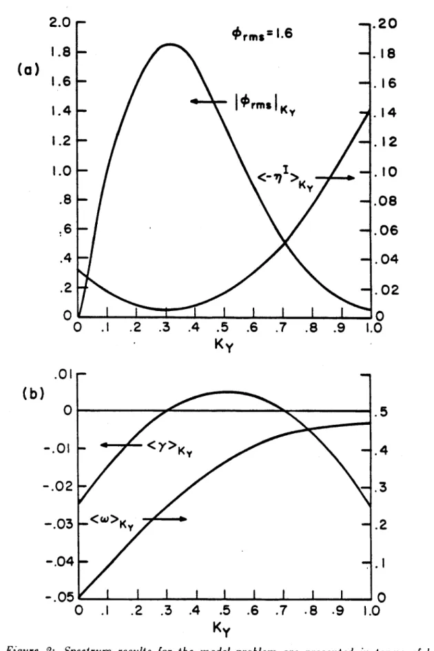
ana-lytic moment method, in dimensionless normalized units, is 0rm, = 1.6. This is in almost

perfect agreement with the quoted numerical results, and is on the order of the

experimen-tal values. In dimensionless normalized units, the average frequency width, (-?,I) ; .02,

found by this moment technique, is much less than the average frequency,

(W)

~ .3. This is

also in agreement with the numerical results of Waltz, but, of course, quite a bit different

from the broad frequency spectral widths observed experimentally. Finally, in Sec. 4.,

a Gaussian frequency function along with a Gaussian wave number function is used to

solve the spectrum equation for a model of electron drift wave dissipation derived in the

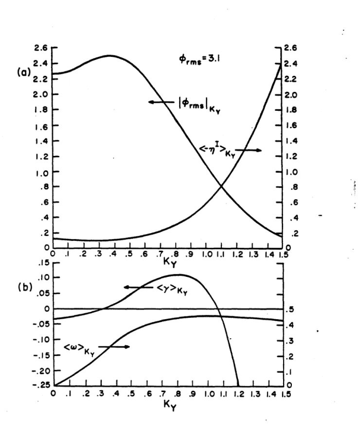
NSA [4]. Using the approximate analytic moment method of solution, in dimensionless

normalized units, the root mean square potential is

krma

3.1. Also, in dimensionless

normalized units, the average frequency width,

(-r7

1 )

~ .3, is on the order of the average

frequency,

(w)

_{z .3. A comparison is made between the model dissipation of Waltz and the}

electron dissipation in the NSA with emphasis on the resulting spectral frequency widths.

It should be noted that the frequency width to frequency ratio is roughly independent of a

growth rate rescaling for the electron dissipation in the NSA. Therefore, the difference in

frequency widths for the two dissipation models cannot simply be attributed to a rescaling

of the growth rate. Consequently, a more detailed analysis of differences in the growth rate

structure for the two models must be considered. The basic point is that the wave number

dependent growth rate for the model problem of Waltz contains a narrow wave number

region with small positive growth rates. Almost any two unstable linear eigenmodes which

beat together form a third nonlinear mode which is stable, where the triplet growth rate

is also stable. Since there are very few unstable triplets to drive up the noneigenmode

frequency spectrum, the resultant spectral frequency widths are small. For the case of the

growth rates derived from this model of electron dissipation in the NSA, every eigenmode,

W

=

wk,

is unstable. Any two eigenmodes with positive y components of the wave vectors

which beat together form a third nonlinear mode which is also unstable. There are many

unstable triplets that drive up and populate the noneigenmode frequencies. It is then

an-ticipated that the solution of the spectrum equations dependent on the electron dissipation

in the NSA will result in large frequency spectral widths. The spectrum results for this

dissipation model, being

e,ms/Te

a 10-2 and an average frequency width on the order

of the average frequency, are in rough agreement with the experimental observations in

A. Spectral Trial Function: Frequency

In a linear eigenmode theory the effective frequency spectrum, for any fixed wave number, is centered about the linear eigenfrequency, wk, with negligible frequency width. In general, however, the spectrum equation is nonlinear so that one expects the frequency spectrum to be centered about a nonlinear frequency, ,f - wk +69 (6b7 is the nonlinear

frequency shift), with the frequency width being 7 -yj+671 (6t( is the nonlinear growth rate shift). Employing these two general physical features of the frequency spectrum, two particular frequency spectral shapes are chosen (the Lorentzian and Gaussian) for the trial functions. This leads to a reduction of the spectrum problem to wave number space. 1. Lorentzian Line Shape

One possibility for the spectral frequency trial function is the very common Lorentzian model. In fact, the Lorentzian frequency function appears to occur naturally in the spec-trum equation. Actually, it will be demonstrated that this is due to the method of renor-malization used to derive the spectrum equations, where the nonlinear complex frequeny,

7

k,w, was introduced. Although superficially there seems to be only one reasonable choice for the frequency trial function (the Lorentzian), it is shown that general choices are possi-ble by changing representation of the spectrum propossi-blem from the calculation of a nonlinear complex frequency, qk,,, and a spectrum, Sk,w, _{to the calculation of a propagator, Gk,,,}

and a spectrum, Sk,w. The use of this alternate representation will not lead to any prac-tical restriction on the form the frequency spectral trial function may assume. In this section, the representation employing the nonlinear complex frequency, ?7k,w, is used. In

the following section, we will develop the other representation.

The spectrum problem [via Eqs. (39) and (40)] is that of calculating the spectrum, Sk,,, and the nonlinear complex frequency, 17k,w. The equation for the spectrum is analyzed

first, followed by that of the nonlinear complex frequency. The starting point is Eq. (39) for the spectrum, where definition (40) has been used,

-i(w

-

2_k,w)Sk,,

f

_dX

_{2Ckk',kSkwISk",wi}

-T Ck,k i,k t CkikIt ,k Skw Sk = [-a,,

+

in',',

}st

(47)

2

_-yk,wSk,W

=

_dX

L4

,k)kI

_{- R (w7}

_~w

_{+ 2l~}

_Ski'W

_,w'ki,wi

I

- 87rCk,k,,k"Ck,,k",kSk,- , 1k', Ski,

(48)

kr(

' k' k",w

It is interesting to note that the real part of the propagator,

Rk, = Gk, + G* 7r (L - ) + (k)2

will take on a Lorentzian form in frequency, if ?lk,w - ik.

In reference to Eq. (48), it should be noted that the right hand side driving terms each contain two spectrum factors, S, and one real propagator factor, R. It will be fouid that the equation for the nonlinear complex frequency will have a triplet driving term containing two real propagator factors, R, and one spectrum factor, S. This symmetry will be even more clear when we examine the alternate representation utilizing the propagator,

Gk,,, and the spectrum, Sk,w. The three factors in each equation physically represent the fundamental triplet interaction found in mode-mode coupling. Parenthetically, in order to integrate the spectrum equation, Eq. (48), over frequency to obtain a wave number spectrum equation, the frequency convolution integrals for the triplet interaction must be obtained. If the spectrum, Sk,w, is taken to be proportional to the real part of the propagator, Rk,,, then the resultant convolution integrals in frequency will combine in such a way that the derived resonance function or interaction time, Ik,k',k", will contain elements of the nonlinear complex frequency, symmetrically for all three waves in a triplet, similar to that found in weak turbulence theory. Consequently, in view of the above arguments, it is a useful simplifying assumption to make an ansatz such that the spectrum is proportional to the real part of the propagator,

Sk,w - SkRk,,, (50)

where the real part of the propagator is normalized to one, f dwRk,L 1.

The spectrum problem is thereby reduced to the evaluation of the normalized spec-trum, Rk,,, and the nonlinear complex frequency, tlk,w, with the subsidiary condition that

Eq. (49) is satisfied. In view of Eq. (49) for the general form of the normalized

spec-trum, Rk,,, a possible choice for the normalized spectral frequency trial function is the Lorentzian,

1-- k r7kW -+ rk.(51)

7r (W - r1R)2 + (r;I)

Inverse Fourier transforming the normalized spectrum, Rk,,, gives

Rk(r) = e-' ]'7+""rl,

(52))

where Rk(r) is the spectral correlation function. The propagator, Gk,,, and its inverse Fourier transform are

Gk,,

1

1

,) and Gk (7)

=

{

,

(53)

27r -i(w - r7k) 'I0, r <

0-where the imaginary part of the nonlinear frequency is assumed to be less than zero, Imr7k =

7

< 0.

The time asymptotic steady state wave number spectrum, Sk, can be obtained by integrating the wave number frequency spectrum, Sk,w, over frequency,

dSk,

J

dw

(21

dydre-i(k y-wr) (q(X

+ yt

+

r)q(x, 0)

dye-ik Y (0(x + y, t)k(x, t)) = Sk. (54) The wave number spectrum, Sk, is independent of time for a stationary turbulent state, which is assumed to exist. The steady state spectral equation in wave number space is then derived by introducing the frequency spectral trial function, Eq. (51), in the spectrum Eq.

(48) and integrating over frequency,

-21

dw'7k,wSk,o

f

dk'dk"6(k -

k'

-

k")[47rC2,k,,kSkSkJ dwRk,J dw'R

,k",,o,

The triplet resonance function is

ReIkk,k"

dwRk,f drRk,,,,R,.

=2,

(56)

7r (AnR)

2

+ (n )

2

where j7T - ??

+

17,

+

, - - k', and use has been made of

Parse-val's power theorem, f dwfeg, = (1/27r) f dtf(-t)g(t), and the inverse transform of a

convolution, f dwe-i" f d='feig _,

f (t)g(t).

The spectral equation in wave number space can now be written in a familiar form,

-2ykSk

f

dX47rReIk,kk,w4Ck k,,,,Sk'Sk"

-

2Ck,k',ksCk',k",kSkSk"},

(57)

where the integrated growth rate is defined as

'1k

E

J

dw-k,wRk,,,

(58)

and f dX = f dkb(k

-

k'

-

k").

In order to complete the coupled set of nonlinear integral equations describing the

spectrum in wave number space, the equation for the nonlinear complex frequency, Ilk,

must be derived. This is obtained by multiplying Eq. (40) for the nonlinear complex

frequency, 77k, by the normalized spectrum, Rk,,, to give,

?kRk,. = fk, Rk,

- if

dX4Ck,kI,k"Ck,k,k2rRkw

f

dw'Gk',,,'Sk",_,L.

(59)

Then integrating Eq. (59) over frequency, which corresponds to the step used in deriving

the wave number spectrum equation, results in

7k

dwf2k,,Rk,,

- if

dX4rCk,k',knCk,k",kSkit

2

J

dwRk,

J

dw'Gk',,'Rk",w-,'.

(60)

Defining the complex resonance function, Ik,k',k", from the term on the right hand side

of Eq. (60) and performing the frequency integrals which are similar to those done in

obtaining Eq. (56), results in

Ik,k',k"

=

2f

dwRk,w

J

dw'Gk',,,

RkI,,w.-w,,

(61)

so that the complex resonance function is

=1 -1 1 -I Ikk'k" = --_RA Re _ReIk,kl,k"T,, ' 7'rN i I (A77R) 2 + (7)2 1 Anr ImIk,k,,k" = R (62) W(ArIR)2 + (11 2 Finally, the equation for the nonlinear complex frequency is

r7k = fk - if dX47rIk,k.,k" Ck,k',k" Ckt,k",kSki, (63)

so that the nonlinear growth rate is

?7 = Yk- dX47rReIk,k',k" Ck,kI,iCk/,k,k Ski,, (64) and the nonlinear frequency is

Rf

r7k = ±k + dX47rImIk,kI,k, Ck,ki,k" Ck',k,k Si, (65)

where we have defined the spectral averaged complex frequency as

f

=

dwT,2Rk,,,

and

Wk

f

dwWk,,Rk,,.

(66)

Using the nonlinear growth rate Eq. (64) in the spectrum Eq. (57), yields a convenient equation for the spectrum,

27 Sk dX47r ReIkka C2,gi i, (67)

-ik

fX4fekl,k"Ck,kI

,k"

Sk' Sk"*

67 This last equation, Eq. (67), demonstrates the physical picture that, in the steady state, the spectrum, Sk, is proportional to the ratio of nonlinear drive (via the SkSk,, term) to nonlinear damping, ?7k'. The nonlinear drive is due to the three wave process where a spectral quanta at k' interacts with one at k" to produce one at k. The nonlinear damping

is a result of linear wave particle interaction plus nonlinear wave-wave interaction, where a spectral quanta at k interacts with a second quanta to produce a third quanta.

If this spectrum problem had been formulated without renormalizing the propagator, as demonstrated in the weak turbulence section, then it would not be possible to integrate for the interaction time, ReIkl,,kI, of the triplets. Some of the triplets are linearly

unstable

(IT = -Yk + IVk

+

YV > 0),

so that the integral would diverge. However, when

the resonance function is defined in this renormalized version of the spectrum problem, the nonlinear growth rates, 77, are nonlinearly coupled to the spectrum [Eqs. (64) and (67)] and can adjust to become negative, tq < 0. In the limit that the nonlinear damping rate is

zero, 77 -+ 0, so that there is no width in the frequency spectrum, the resonance function

implies a nonlinear frequency, 77, selection rule, since ReIk,k,," _ -+ yq) =

(

- ],- 1

).

This produces an expansion about spectra of nonlinear real frequency that satisfy the above selection rule, and is similar to the linear real frequency expansion found in weak turbulence theory.

An equation similar to Eq. (63), for the nonlinear complex frequency, was derived by Kraichnan [13] while searching for an approximate solution of the wave number spectrum,

by using the time domain DIA equations in the fluid turbulence limit (Isw lk). At first, Kraichnan [13] did not obtain the three wave symmetric resonance function, Eq. (12). However, by using a Fokker-Planck type formulation of the spectrum problem, Edwards

[14)

obtained this symmetric result. Later, Kraichnan

[15]

developed a revised version of the DIA, which employed a semi-Lagrangian-Eulerian formulation, and produced the symmetric resonance function, Eq. (62).

In the above reduction of the spectrum problem to wave number space, the derived wave number dependent linear complex frequencies, 0k, involve frequency moments over the spectrum, k - f dwfg,,Rk,w. For the fluid limit of the spectrum problem, the linear frequency, wk, and growth rate, ay, are unchanged in the wave number reduced spectrum problem, since f dwRk,, = 1. For the general plasma spectrum problem, where the drift wave growth rate is a function of frequency as well as wave number, the frequency moment integral presents a problem if the Lorentzian frequency function is used. The width of a Lorentzian function is usually defined as the width at half maximum, Rk,,7 ±width

1/2R,,7n -> width = r71, although the variance or higher moments of the Lorentzian are not convergent, f dwW2Rk,, - oc.

The problem associated with the Lorentzian can be traced back to the original renor-malization prescription of the potential fluctuation equation, where the nonlinear complex