Analysis of biomarker candidates from plant lipid inputs into Galapagos lacustrine sediments

Analysis of Biomarker Candidates from Plant

Lipid Inputs into Galapagos Lacustrine Sediments

by

Katharine Ricke

Submitted to the Department of Earth, Atmospheric and Planetary

Science

in partial fulfillment of the requirements for the degree of

Bachelor of Science in Earth, Atmospheric and Planetary Science

at the

MASSACHUSETTS INSTITUTE OF TECHNOLOGY

May 2004

\'-yAe

2oLw~I

@

Massachusetts Institute of Technology 2004. All rights reserved.

A u th o r . . . .

Department of Earth, Atmospheric and Planetary Science

May 10, 2004

Certified by.

Signature redacted

...

Julian Sachs

Assistant Professor

Thesis Supervisor

Accepted by ...

Signature redacted

Sam Bowring

Chairman, Committee on Undergraduate Program

0.

Analysis of Biomarker Candidates from Plant Lipid Inputs

into Galapagos Lacustrine Sediments

by

Katharine Ricke

Submitted to the Department of Earth, Atmospheric and Planetary Science on May 10, 2004, in partial fulfillment of the

requirements for the degree of

Bachelor of Science in Earth, Atmospheric arid Planetary Science

Abstract

Paleoclimatological investigations into past precipitation and temperature patterns in regions of the tropical Pacific may be the key to resolving scientific disputes about the effects of global warming on the magnitude and frequency of the El Nifio/Southern Oscillation (ENSO) phenomenon. Plant lipids identified in the sediment record of lakes in regions of high ENSO activity can act as biomarkers to reconstruct past precipitation patterns by measuring the D/H ratios preserved in these compounds to observe the local climate changes with global temperature variations. Twelve plant species and two sediment samples from in and around El Junco lake catchmernt on Sari Cristobal in the Galapagos Islands were solvent extracted, identified and quantified using gas chromatography arid mass spectrometry. The analysis revealed evidence for significant aquatic and terrestrial vascular plant inputs to lake sediments. High concentrations of unsaturated C16 and C18 fatty acids were found in all plant samples, but these compounds appear to be degraded significantly in the sediment record. ri-Alkane distributions suggest a strong hydrocarbon contribution from submerged and floating plants. Additionally, a terrestrial biomarker, fernene, was identified. The information in this study should be a helpful guide for further biomarker identification efforts at the El Junco lake and in other tropical crater lakes.

Thesis Supervisor: Julian Sachs Title: Assistant Professor

Acknowledgments

First and foremost, I would like to thank my academic and thesis advisor, Assistant Professor Julian Sachs, both for helping me along in my academic career at M.I.T. over the past three years and for allowing me to work in his lab despite my sometimes short attention span. He came up with this project for me and it's been an amazing learning experience. I would also like to thank Dr. Paul Colinvaux of MBL for his generous contribution of time and plant samples, not to mention a great tour of Woods Hole and an exciting ride in his fancy car; as well as Dr. Alan Tye of the Charles Darwin Research Station for sample advice and several generous attempts to procure fresh plant samples for this project. Most of all, though, I am indebted to Dr. Rienk Smittenberg, who advised and collaborated with me through every step of this project. I cannot thank him enough for his fantastic guidance and patience.

I want to thank my parents for supporting my education and indulging me in

my eccentricities over the years. This applies especially to my decision to come to M.I.T., even though they thought was a terrible idea. It all turned out alright in the end (I think)! Thanks so much to MattX for help with all the many, many technical difficulties associated with the production of this ITEX(!) document, not to mention for keeping me alive and sane throughout the process. You're the best! Thanks to Gretchen for proof-reading. Thanks to Teri and Marc for making me go out instead of working all the time. And indeed, a special thanks to the other half of the pika Thesis Procrastinators Support Group, Shefali.

Last, but not least, my gratitude is heartily extended to Queen and David Bowie for writing and recording the song "Under Pressure", without which this thesis may

Contents

1 Introduction

1.1 El Nifio-Southern Oscillation (ENSO) . . . .

1.2 The Galapagos Islands and the El Junco Lake . . . .

1.3 Biornarkers and Reconstruction of Paleoclimate . . .

1.4 Precipitation Patterns and Hydrogen Isotope Analysis 1.5 T hesis O utline . . . .

2 Methods

2.1 Sam pling. . . . . 2.1.1 Plant Sam ples . . . . 2.1.2 Sediment Samples . . . . 2.2 Lipid Extraction and Derivitization . . . . 2.2.1 Plant Lipid Extraction . . . . 2.2.2 Sediment Extraction . . . . 2.3 GC and GC-M S . . . .

2.4 Identification and Quantitation . . . .

3 Results 3.1 Lipid 3.1.1 3.1.2 3.1.3 3.1.4

Content of Twelve Plant Species Fatty Acids . . . . Hydrocarbons . . . . n-Alkanols . . . . Sterols . . . . 13 14 14 15 17 18 19 19 19 21 22 22 23 24 24 25 25 25 29 29 30

Diols and Midchain alcohols . . . . Contamination, Coelutions, and Errors Content of the El Junco Sediment . . .

Fatty acids . . . . Hydrocarbons . . . . K etones . . . . A lcohols . . . . Sterols . . . . 4 Discussion 4.1 Fernene:

An Indicator for Terrestrial Plant Input . . . 4.2 Observations on Fatty Acid Distributions . . 4.2.1 C1 6 and C18 Fatty Acid Abundances

4.2.2 Disparity in Fatty Acid Distributions 4.2.3 Palmitic Acid as Potential Biomarker 4.3 Parsing Terrestrial and Aquatic Inputs . . . 4.3.1 Variations in n-Alkane Distributions 4.3.2 Variation in Sterol Distributions . . . 4.4 Other Observed Anomalies . . . .

41

. . . . 4 1

. . . . 42

. . . . 4 2

in Plants and Sediment . 44

. . . . 44 . . . . 4 5 . . . . 4 6 . . . . . . . . . 47 . . . . . . . . . 4 7 5 Conclusions 5.1 O n Biom arkers . . . .

5.1.1 Fernene and Terrestrial Plant Input . . . .

5.1.2 n-Alkanes and Aquatic Plant Input . . . . 5.1.3 The Ubiquity of Palmitic Acid . . . .

5.1.4 Preferential Degradation and Non-Plant Inputs 5.2 On Obtaining Quality Plant Lipid Data . . . .

5.2.1 Controlling Sample Quality . . . .

5.2.2 Research Techniques . . . . 5.3 Suggestions for Further Study and Closing Thoughts .

3.1.5 3.1.6 3.2 Lipid 3.2.1 3.2.2 3.2.3 3.2.4 3.2.5 . . . 30 . . . 31 . . . 32 . . . 32 . . . 33 . . . 33 . . . 33 . . . 34 49 . ... 49 . . . . 49 . . . . 50 . . . . 50 . . . . 5 1 51 51 52 . . . . 52

5.3.1 The Quest for Viable Aquatic Biomarkers . . . . 52 5.3.2 T he Big Picture . . . . 53

List of Figures

1-1 The ENSO Precipitation Anomaly and the Galapagos Islands . . . 15

3-1 Typical GC-MS Total Lipid Extract Chromatograrn with Compounds D esignated . . . . . 28

3-2 _{Fatty Acid Concentrations . . . . 35}

3-3 n-Alkane Concentrations . . . . 36

3-4 n-Alkanol Concentrations . . . . 37

3-5 Sediment TLE Chromatogram . . . . 38

3-6 Concentrations of Sediment Compounds: Fatty Acids, Alcohols, n-Alkanes, and 2-Methyl Ketones . . . . 38

3-7 The is the hydrocarbon fraction of the sediment total lipid extract. Numbers correspond with n-alkanes. . . . . 39

3-8 Chromatogram for Hydrocarbon Fraction of El Junco Sediment . . . 39

3-9 Chromatogram for Alcohol Fraction of El Junco Sediment . . . . 39

4-1 Comparison of TLE and Rinse Fraction Chromatograms for C. weath-erby an a . . . . 43 4-2 n-Alkane Distribution Comparison Across Plant Groups and Sediment 46

List of Tables

2.1 Plant sample information. . . . . 21 3.1 TLE Compound Concentrations for Twelve Plant Samples. . . . . 26 3.2 Saponified TLE Neutral Fraction Compound Concentrations for Five

Chapter 1

Introduction

In the context of current debates about global warming, many scientists have hypoth-esized that with a rise in global average temperatures there will be a corresponding increase in number and severity of extrene climate events. Because of the severe flooding and droughts associated with the El Nifio-Southern Oscillation (ENSO) dis-ruption, the social and economic implications of increased duration or magnitude of the phenomenon are tremendous. Certain researchers have theorized that under the effects of global warming, El Nifio-the disruption of the ocean-atmosphere system in the tropical Pacific that causes temperature and precipitation anomalies-will become more pronounced [25, 24]. Observational paleoclimatological research examining past sea surface temperatures in the eastern equatorial Pacific indicates the contrary. Ac-cording to this research, the magnitude of sea surface temperature (SST) anomalies seems to diminish with warmer overall global temperatures [17]. In order to better understand the effects changing global temperatures have on El Nifio, more past cli-mate data is needed from those regions most affected by the ENSO phenomenon. This paper is a preliminary step in efforts to reconstruct precipitation patterns within one such region of high ENSO activity. Through identification of aquatic and terrestrial plant lipid inputs into lacustrine sediment, potential biomarkers may be identified for reconstruction of past water balance through deuterium/hydrogen (D/H) ratio analysis.

1.1

El Ninio-Southern Oscillation (ENSO)

The ENSO phenomenon is the result of an aperiodic ocean-atmosphere fluctuation that causes temperature and precipitation anomalies in several regions of the equa-torial Pacific. Under normal climate conditions, the easterly trade winds cause warm ocean water to "pile up" in the western tropical Pacific, leaving a relatively cold de-pression and shallow thermocline in the eastern equatorial along the coast of Central and South America. During an El Nifio event, these winds relax causing warm waters to flow into the eastern Pacific, increasing atmospheric convection in the East and further exacerbating the collapse of the trade winds. The results of this collapse have major effects on climate patterns all over the globe [2]. Still, the effects of ENSO are most heavily concentrated within several distinct geographical nodes across the trop-ical Pacific [19]. It is within these core regions that evidence for past ENSO activities should be most pronounced.

Two of the most recent El Niio events-those occurring in 1982/83 and 1997/98-were the most intense in over a century; possibly as a result of rising greenhouse gas concentrations in the atmosphere [11]. Several models suggest ENSO behavior is closely linked to Milankovitch orbital forcing and climate cycles [4], but theoretical understanding of such variability is relatively poor. Thus one of the best ways to un-derstand how El Nifio may change under altered future climatic conditions is through paleoclimatological investigations of potential ENSO activity throughout glacial and interglacial climate periods.

1.2

The Galapagos Islands and the El Junco Lake

Darwin's famous desert islands, the Galapagos, lie directly along the equator at the edge of the cold tongue of the eastern equatorial Pacific. The typically arid climate of the island is inundated by a large positive precipitation and temperature anomaly during an ENSO event. [19] On the eastern-most island of San Cristobal, a closed basin crater lake, El Junco, lies at the top of an inactive volcano. Closed basin lakes

are particularly good targets for past precipitation studies because their often simple evaporation-precipitation hydrological systems and relatively small volume creates an environment with high sensitivity vis-h-vis water chemistry parameters. Another advantage of the El Junco crater lake is the lack of massive biological diversity that could be a hindrance in attempts to identify species-specific biomarkers in sediments in most of the world. The lack of plant species diversity in the highlands of the Galapagos Islands makes a thorough comparative investigation of sediment and species samples

possible [8].

THE GALAPAGOS

f~appr.,1PRocnoysit CIUA O 'GENOVESA_

.0 FERNAAGIN El NlrEl A x 1 SANTA CRUZ2 I0- FLOREAN SAN CRISTOBAL * -JUNCO

Figure 1-1: The largest El Nifio precipitation anomalies are concentrated in nodes across the equatorial Pacific. The Galapagos Islands (inset) lie within one such node. The El Junco crater lake is at the top of a mountain on the eastern-most island of San Cristobal. (Figures adapted from http://www.cdc.noaa.gov/ENSO/ [19] and

Colinvaux (1968) [6].)

1.3

Biomarkers and Reconstruction of Paleoclimate

Aquatic sediments are a long established source of paleoclimatological information. By identifying and quantifying a variety of mineralogical, biochemical and fossil in-dicators preserved in the sediment record, climate characteristics such as SSTs, pre-cipitation magnitudes and biological productivity can be reconstructed. Only a small

fraction- 0.1-1%-of the biological material produced in an aquatic environment makes it into the sediment record [10]. Chemical and biological processes within the lake degrade the primary products of plant growth. Yet some forms of organic matter are less vulnerable to degradation than others. CaCO3 traces from diatoms or SiO4 produced by foraminifera can be used to gauge past environmental conditions such as salinity, temperature, species composition of nutrient level-all factors effected by climate variations. Pollen and macrofossil records have been a popular source for information about vegetation in lacustrine sediments [13]. A profile of alteration in microfossil remains of pollen grains from the submersed water fern, Azolla micro-phylla, and was taken from the El Junco lake sedimentation and used to reconstruct periods of relative moist and arid climate that corresponded with glacial and inter-glacial variations in global climate [7]. However, the bacterial and algal components, and a large amount of non-recognizable organic matter, is outside the analytical win-dow of such studies. Lipid analysis provides the opportunity for a comprehensive view of all of the biological components of sedimentary input and the variations therein that are influenced by environmental change.

One of the most versatile indicators of past climate conditions is the biolipid content of sediment samples. Living organisms produce a wide variety of lipids-substances that can be extracted from organic matter by nonpolar solvents, such as hexane. Though lipids make up only a small fraction of the total biomass produced, in depositional environments they are better preserved than sugars and proteins [10] and easier to analyze than large macromolecular components like cellulose and lignin. Thus through the identification and quantification of specific lipid components, called biomarkers, organic matter in sediment can be used to reconstruct the environmental conditions under which it was originally produced. [9].

Examples of molecules that can be lipid biomarkers include fatty acids, n-alkanes, triterpenoids, and alcohols. Well-known biomarkers from vascular plants are long-chain n-alkanes (C2 5-C3 1). These compounds exhibit a strong bimodal

distribution-with odd carbon numbered components occurring in far more abundance than even-numbered components-which are part of the waxy surfaces of terrestrial plant leaves

[10]. Ficken et al. (2000) compared the distributions of all n-alkyl lipids (n-alkanoic

acid, n-alkanols and n-alkanes) between a number of plant species, both aquatic and terrestrial, and sediment samples from lakes on Mt. Kenya in East Africa and found a correlation between the carbon chain length of n-alkanes and the environmen-tal growth conditions of the plant (submerged, emergent or terrestrial). Correlative analysis between lacustrine sediments and plant samples is feasible by way of other biomarkers as well. Baas et al. (2000) differentiated the lipid abundances across several categories for twelve species of peat moss through total lipid extraction and gas chromatography-mass spectrometry analysis and used compound distributions to identify a "chemotaxonomic fingerprint" for the species in peat bogs. A great number of studies have identified correlations between lipid content of vascular plant inputs and sediment deposits.

1.4

Precipitation Patterns and Hydrogen Isotope

Analysis

The water balance of a small-basin aquatic body changes markedly during an El Nifio event, within a node of high ENSO activity, with precipitation increasing rel-ative to evaporation. Sternberg (1988)[23] showed that lipids of submerged aquatic plants record deuterium/hydrogen (D/H) ratios of environmental water. By looking at relative abundances of deuterium to normal hydrogen in lipids one can evaluate the magnitude of evaporative loss of water from the lake relative to gain via precipitation. Sauer et al. (2001) used algal sterols in lacustrine sediments to reconstruct past iso-topic characteristics of the lake's water. Huang et al. (2002) examined the deuterium isotope abundance, or 3D, of the ubiquitous lacustrine sediment compound, palmitic acid, in conjunction with fossilized pollen to show a correlation in the JD and pollen-inferred temperature [15]. Through identification of lipids characteristic to abundant submerged water plants, it may be possible to reconstruct the water balance of El Junco, and hence El Nifio frequency and intensity during the past 30,000 years.

1.5

Thesis Outline

The goal of this paper is to draw a correlation between the lipid composition found in the preliminary analyses of available El Junco lacustrine sediment samples and the lipid content of samples of abundant aquatic and terrestrial plants in and around the El Junco lake. Through careful comparative spectrographic analysis, promising biomarkers are identified for D/H isotope ratio analyses of sediment samples to be collected in an upcoming expedition to El Junco. The information in this thesis and the recommendations should prove helpful to further comparative study of plant inputs and sediment for the El Junco lake in the future.

In Chapter 2, the methods for the extraction, identification and quantification of lipids from plant samples collected from the El Junco catchment are described and contrasted with the methods employed by Dr. Rienk Smittenberg, a post-doctoral researcher at M.I.T., in obtaining the same lipid information from El Junco sediment samples. Chapter 3 summarizes the results of the study by describing the general character of the lipid distributions in twelve plant samples and one sediment sample. In Chapter 4, the features of the plant lipid extracts are compared to those of the sediment sample and some of the most remarkable features of the data are are further detailed. Examples of such features include the similarities and differences of distri-butions in the fatty acids and n-alkanes of the plant and sediment samples, and the identification of a terrestrial plant hydrocarbon biomarker, fernene. Finally, Chapter 5 highlights the most important observations about the lipid content of the plant samples and lacustrine sediment and makes suggestions for future investigations into biomarker identification for the El Junco lake, as relevant to the quest to reconstruct past water balance for the lake.

Chapter 2

Methods

In order to compare lipid components of the sediment with those of actual plant sam-ples, both types of samples were extracted using organic solvents and measured by gas chromatography and mass spectrometry. With guidance from Dr. Rienk Smitten-berg, the author was responsible for extraction and measurement of lipids in plants samples, while Smittenberg performed the corresponding analyses on the sediment samples. His methods are described in subsections 2.1.2 and 2.2.2, following the author's corresponding methods description, for convenient comparison.

2.1

Sampling

2.1.1

Plant Samples

While fresh plant samnples-freeze-dried and sent directly from the Galapagos-would have been ideal for the analysis in the study, acquisition of such samples proved impossible on the timescale available for the project. Thus, conventional herbarium samples were used. All plant specimens were originally collected from the El Junco lake basin catchment on San Cristobal in the Galapagos; and were generously donated by Dr. Paul Colinvaux from his private herbarium.

All samples were collected by Colinvaux; primarily in July of 1966, with some

polyethylene bags. As soon after collection as possible, specimens were sorted, folded between sheets of old newspaper and stacked and pressed between aluminum dividers in hand-operated screw presses. The air-dried samples were shipped to Columbus, Ohio for final preparation by a trained herbarium curator and divided into two sets. One set was shipped to Dudley Herbarium at Stanford University for identification arranged by Ira Wiggins and the second was retained by Colinvaux. These specimens were mounted with glue to standard herbarium sheets or, in some cases placed within paper envelopes glued to herbarium sheets, and stored in manila folders in a steel herbarium cabinet. The cabinet remained in an air-conditioned laboratory in Colum-bus until 1990, after which it was shipped to the Smithsonisan Tropical Research Institute (STRI) in Panama, where it remained in an air-conditioned laboratory until 1998. It was then shipped to Woods Hole, Massachusetts, where it has since remained in the basement of a cottage. In 37 years of storage, the only known treatment to the cabinet was the introduction of the insect repellents, camphor or napthelene (moth balls). Subsamples were taken from the specimens stored in this cabinet by the author in Woods Hole in January 2004 [5].

Samples were taken of twelve aquatic and terrestrial native plant species found in abundance in and around the El Junco lake. Species of aquatic or semi-aquatic plants sampled include the water fern, Azolla microphylla; the submersed carnivorous water plant, Utricularia _{foliosa; the bed-forming reed, Eleocharis mutata; the semi-aquatic,} reed bed-dwelling herb, Hydrocotyle galapagenrsis, also found in abundance in the pas-ture outside the crater; and the submersed water plant, Najas guadalupensis-found not in El Junco lake, but rather in divertica of streams running down from the crater. Terrestrial plants sampled include the abundant tree fern, Cyathea weatherbyana; the 2-3 meter tall flowering shrub, Miconia robinsoniana; the flowering herb, Cuphea carthagenensis, and the small flowering shrub, Ludwigia leptocarpa, that both grow on the marshy flat next to the lake; the weed, Polygonum punctatum, which grows on patches of lava mud within the catchment; and the invasive guava tree species, Psidum galapageium, which has become very abundant on the island over the past half century.

ID Species Environment Found in catchment? Glue?

A Utricularia foliosa aquatic, submerged Y N

B Azolla mricrophylla aquatic, submerged Y N

C Najas guadalopersis aquatic, submerged N N

D Eleocharis mutata aquatic, rooted Y Y

E Hydrocotyle galapagensis semi-aquatic, rooted Y Y

F Cyathea weatherbyana terrestrial Y Y

G Ludwiga leptocarpa terrestrial Y N

H Miconia robinsoniana terrestrial Y N

I Cuphea carthagenensis terrestrial Y Y

J Polygunum punctaturn terrestrial Y Y

K Trichomanes Krausii terrestrial N Y

L Psidum galapageum terrestrial N N

Table 2.1: Plant samples analyzed listed with environmental information and indica-tion of glue contaminaindica-tion.

At the time of subsampling in January 2004, specimens were intact, but aged to varying degrees from forty years of handling. It is likely that specimens accumulated some amount of extraneous biomass as a result of collection, storage and reference techniques that were not ideal for samples intended for organic geochemical analysis. In addition, though subsamples were taken from the envelopes containing glue-free surplus specimens whenever possible, half of the samples had been mounted with glue to standard herbarium sheets, and it proved impossible to completely remove all said glue from the surface of the samples.

2.1.2

Sediment Samples

Sediment cores were taken in 1972 by Colinvaux using a modified Livingstone piston corer, and portions were subsampled into 1 cm3 _{parts. After transport they were}

stored in glass vials at 4C in Columbus, Ohio; and after 1990, at Northern Kentucky University. During the years, the subsamples slowly desiccated. Two sediment sam-ples, of 15 cm and of 208 cm core depth, respectively, were sent to MIT for biomarker analysis [22].

2.2

Lipid Extraction and Derivitization

2.2.1

Plant Lipid Extraction

Any visible remnants of glue on the surface of the leaves samples was removed with a set of tweezers and reserved for analysis. Stems and non-leaf material were discarded.

All dry samples were weighed and rinsed with dichloromethane to remove surface

contaminants and residues. These rinse fractions were then reserved for further anal-ysis and the samples were crushed and packed with sand for lipid extraction. All samples were extracted using a soxhlet apparatus for approximately 15 hours in a dichloromethane/methanol (DCM:MeOH 9:1 v/v) mixture. A blank experiment and glue sample were run concurrently. After extraction, a 5oa-cholestane standard was added to all samples (approximately 1 pg/10 mg dry weight of sample) for quan-tification purposes. The remaining plant material was reserved for further analysis through saponification. Solvents were removed by evaporation under nitrogen gas using a Zymark Turbovap LV (Caliper Life Sciences, Hopkinton, MA, USA) and the residues transferred to 4 mL vials using DCM.

Aliquots of total lipid extracts (TLEs) and sample rinses, equivalent to 25-50 mg of dry plant weight (or 1 of the sample if total dry weight was less than 50 mg), were dried over pipette columns of anhydrous Na2SO4. To remove highly polar compounds they were subsequently eluted over pipette columns filled with 5% deactivated silica

60 with ethyl acetate. All solvents were evaporated under a stream of nitrogen and

the residues were silylated with 5 ptL of bis(trimethylsilyl)trifluoroacetamide (BSTFA) and 5 pL of pyridine for 20 minutes at 600C to convert alcohols and acids to their

trimethylsilyl ethers. Derivitized samples were then diluted in ethyl acetate for gas chromatography (GC) and gas chromatography-mass spectrometry (GC-MS).

The TLEs and remaining plant material of five samples identified for particular ecological importance (abundance and/or submersed aquatic growth environment) in the study, A. microphylla, U. foliosa, E. mutata, C. weatherbyana, and M.

robinso-niana, were subjected to saponifaction. Aliquots equivalent to 25-50 mg dry weight

ml 1 N KOH solution (MeOH:H20 95:5 v/v) for two hours. The resultant extracts

were transferred to Teflon centrifuge tubes, shaken over distilled water and hexane and centrifuged three times. Neutral fractions were recovered by reservation of the hexane after each run. Acid fractions were recovered in an identical manner, after acidification of the alkaline solution with HCl to a pH level less than 3. Residues of the extracted plant leaves were saponified in the same way as the TLE fractions, resulting in neutral and acid fractions. All fractions were prepared for GC and GC-MS as described above. For quantification, 5a-cholestane standard was added to the hydrolyzed TLE acid fractions and to the saponified residue fractions.

2.2.2

Sediment Extraction

Sediment samples were freeze-dried and weighed. Except for small amounts kept as reference material, the sediments were extracted and prepared for GC and GC-MS analysis in a similar manner to that described for the plant samples. To transform fatty acids into their corresponding methyl-esters, half of the total lipid extract was dissolved in a mixture of BF3 (14%) in methanol and heated to 60'C for 5 minutes.

After addition of H20, lipids were extracted in a separatory funnel with DCM and

dried over a pipette column filled with anhydrous MgSO4. The fractions were

subse-quently eluted over 5% deactivated silica and derivatized with BSTFA as described above. The other half of the TLE of the sample from 15 cm-depth was saponified in a fashion similar to the methods described for the plant samples, and separated into an acid and a neutral fraction. The acid fraction was treated with BF3/methanol

to convert the fatty acids into their corresponding methyl esters. Both the acid and neutral fractions were separated into 4 fractions over a pipette column filled with 5%

deactivated silica, using subsequently hexane (hydrocarbons), hexane:ethyl acetate (9:1 v/v) (neutral fraction: ketones; acid fraction: fatty acid methyl esters),

hex-ane:ethyl acetate (8:2 v/v) (neutral fraction: alcohols; acid fraction: hydroxy-fatty acid methyl esters), and ethyl acetate (rinse) as eluents. The fractions were prepared

for GC and GC-MS analysis using BSTFA as described above. Compounds were quantified by injecting known volume fractions (1/500) into the gas chromatograph,

and comparing the integrated peak areas in the chromatograms with peak areas of a standard mixture of four compounds with known concentration, which were analyzed immediately before and after the samples.

2.3

GC and GC-MS

Gas chromatography was performed using an Agilent 6890N Network GC System equipped with a PTV injector and monitored with a flame ionization detector. A CP-Sil 5 CB fused silica capillary column (60m x 0.32mm, 0.25pm film thickness) with helium as a carrier gas was used for separations. Samples were injected and held at 70'C for two minutes. The temperature was raised at 20"C/min up to a temperature

of 130'C. The temperature was then raised to 320'C at the rate of 44C/min and held for twenty minutes. Gas chromatography-mass spectrometry was performed on a Hewlett-Packard 6890 instrument with an Agilent 5973N Mass Selective Detector operated in electron ionization mode at 70 eV and with a mass range of rn/z 50-800, using the same silica capillary column, carrier gas, and temperature program as the GC.

2.4

Identification and Quantitation

Lipids were identified from the GC-MS data with the aid of GC-MS Enhanced Data Analysis software and gas chromatographic reference literature, as well as AMDIS-Chromatogram with NIST MS Search software. Components were then quantified by integration of peak area generated by the gas chromatograph and comparison with the cholestane standard peak.

Chapter 3

Results

Twelve total lipid extracts (TLEs), five sets of neutral fractions (TLE and residue), five sets of acid fractions, one glue extract and a procedural blank were analyzed for lipid content using GC-MS data to identify compounds and GC to quantify each identified peak. A typical TLE gas chromatogram is shown in Figure 3-1. The numbers designating the peaks refer to the compounds identified and listed in Table 3.1. Lipid quantities for the 5 TLE neutral fractions are listed in Table ??. Biomarker

content of the plant samples is organized by chemical classification in the first section of this chapter. Additionally, as the results of Dr. Smittenberg's sediment extractions are unpublished at this time, the sediment data are summarized in the second section of this chapter. Due to time constraints on the project, the results summarized below do not represent an exhaustive analysis of the data, but rather an organization of the most obvious results and those considered most interesting and/or important.

3.1

Lipid Content of Twelve Plant Species

3.1.1

Fatty Acids

The n-alkanoic acids, or fatty acids, were the most abundant free lipids extracted from the samples of all plants species. The summed concentrations vary between 413 to 2600 ug/g dry weight of the sample. Especially abundant in all samples

Compound Species ID A B C D E F G H I J K L Fatty Acids n-Alkanoic Acids 1 16:1 2 16 3 17 4 18:2 5 18:1 6 18 7 19:1 8 20 9 21 10 22 11 23 12 24 13 25 14 26 Sum Alcohols n-Alkanols 15 phytol 16 19 17 20 18 22 19 24 20 26 21 28 22 30 Sum Midchain Alcohols 23 31 24 33 Sterols 25 cholesterol 26 28:1 27 29:2 28 29:2 stigma-29 29:1 31 29:1 sito-32 29 -sito 33 30 lano-Sum Diols 34 29-9,21 35 30-11,20 Hydrocarbons n-Alkanes 36 n23 37 n24 38 n25 39 n26 40 n27 41 n28 42 n29 43 n30 44 n31 45 n33 Sum Triterpenoids 46 fernene 47 dehydroabietic acid 23 1068 54 122 376 462 102 137 96 97 61 * 2598 12 1054 21 21 151 225 107 33 10 154 12 25 1824 41 111 * 9 18 151 27 62 120 153 174 73 520 14 51 288 353 24 1151 27 * 250 214 106 96 * 58 30 1955 17 18 1063 875 21 20 35 123 204 56 159 145 39 38 63 48 4 25 77 32 17 -21 * 1721 1381 - 28 -- 20 -- - 5 - - 57 - - * 59 1148 12 19 252 167 62 17 13 26 * * 1776 18 1380 23 56 281 205 48 * * * 28 30 2069 * 15 212 334 6 11 14 56 59 124 42 85 19 -22 28 * 6 20 51 3 14 11 23 * 8 4 21 413 777 9 65 3 -- - 2 -- - 6 -- - -- 11 - - -48 61 9 65 22 8 4 15 380 562 495 17 20 17 47 38 51 59 222 76 60 83 154 37 105 37 -* -51 39 40 15 16 12 50 43 13 - 8 -27 13 -752 1152 909 - 7 42 -* 20 - -- 10 -20 18 42 - - 78 - 91 199 27 441 -- - 39 -186 141 86 605 13 -153 22 -731 27 328 731 188 198 399 198 399 -- 298 - 146 35 29 31 29 19 * * 30 -23 -20 -- - 15 109 123 581 - 10 * 18 16 21 - 12 - 17 * - - 4 7 17 10 - -- -*-- - 5 * * * -- - - - * * -- - 5 * * 25 15 - - - - - 24 -- - 6 10 - 33 128 94 - - - - 240 324 - 12 32 10 49 9 -* 12 10 * -6 32 26 - 15 -- 19 263 - - 55 17 125 461

= coelutes, '-' = not identified

Table 3.1: The lipid identities and concentrations for the Total Lipid Extracts. The values represent Mg of the given compound/g of dry weight of the plant sample. Asterisks denote compounds that coelute. Dashes indicate compounds that were not detected in the given sample.

Compound Species ID A B D F H Alcohols Midchain Alcohols 23 31 89 7 * 19 116 28 * * 19 21 27 95 29 18 * 11 15 8 * 81 53 104 33 - 50 112 126 48 390 110 235 - 6 - 543 160 305 - 105 379 889 266 296 158 Hydrocarbons n-Alkanes n23 n24 n25 n26 n27 n28 n29 n30 n31 n33 Sum Triterpenoids fernene

Table 3.2: The lipid identities and concentrations for the saponified neutral fraction of the TLEs of five selected samples. The values represent pg of the given compound/g of dry weight of the plant sample. Asterisks denote compounds that coelute. Dashes indicate compounds that were not detected in the given sample.

15 16 17 18 19 20 21 22 n-Alkanols phytol 19 20 22 24 26 28 30 Sum 323 25 48 42 27 6 13 484 24 2 5 11 13 15 70 25 26 27 28 29 31 32 33 Sterols cholesterol 28:1 29:2 29:2 stigma-29:1 29:1 sito-29 b-sitcf 30 lano-Sum Diols 34 29-9,21 35 30-11,20 204 21 231 13 * * 27 29 24 21 36 37 38 39 40 41 42 43 44 45 46 * 19 18 13 10 9 10 * 8 6 4 9 7 53 * 10 13 9 12 44 60 113 255

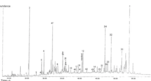
Abundance 2 47 34 32 6 12 35 + _23~ 19 26 42 4 25 20.00 25.00 30.00 3500 40.00 45.00 so00 500 Time--_>

Figure 3-1: Typical Chromatogram shows the Total Lipid Extract results for Azolla

microphylla. The numbers correspond to the compounds listed in Table 3.1.

was palmitic acid, the unsaturated C1 6 fatty acid. In all species, palmitic acid is

at least twice as abundant as any other fatty acid and often the most abundant compound in the total lipid extract (see Figure 3-2). Also abundant were saturated and unsaturated C18 fatty acids; and even-numbered saturated compounds C_{2 2}-C₂₆

were dominant over counterparts with odd carbon numbers. Most rinse fractions showed fatty acid peaks, as well, with distributions generally proportional to those found in the total lipid extracts, though much smaller. Submerged aquatic plant rinse fractions appear to have slightly higher fatty acid peaks proportionally than terrestrial plants do, though the large variations in contamination levels and sample quality make this observation impossible to quantify. In general, the peaks of major contaminants, such as glue molecules and dehydroabietic acid were much larger in the rinse fractions than the fatty acid peaks, the exception to this being in samples with very small or imperceptible levels of glue and paper contamination.

3.1.2

Hydrocarbons

n-Alkanes

With the exception of P. galapagaeum(L), all plant species contained relatively small amounts of n-alkanes. Total concentrations varied between 17 and 125 Pg/ g dry weight. Most species showed either a unimodal or weakly bimodal distribution (see Figure ??). Aquatic plants generally showed a weaker bimodal distribution than terrestrial plants. This may be due to higher vulnerability to contamination from newspaper ink during drying. Ficken et al. (2000) found that lipid extractions from newspaper produce a smooth unimodal n-alkane distribution centered around n-C26. Additionally, the C25 alkane coeluted with another compound in nearly every sample.

The only two specimens to show the strongly bimodal distribution associated with vascular plants were P. galapageum and M. robinsoniana(H). The terrestrial plant, P.

galapageum, had a high total ri-alkane concentration of 461pg/g dry weight, with C29

and C3 1 peaks that were among the largest compound peaks in the chrornatogram.

This may be explained by the specimen's waxy leaves. Strong bimodal long-chain n-alkane distributions are associated with waxy leaf surfaces.

Triterpenoids

The triterpenoid, fern-9(11)-ene (46), was found in considerable abundance in the TLE and neutral TLE fraction of the C. weatherbyana(F) lipid extracts. The concen-trations were measured at 240 and 255 pg/ g dry weight, respectively. It was present in the saponified neutral residue fraction as well, in much smaller abundance. Fernene was not found in any amount in any of the other plant extracts. It is a compound that has only been isolated in ferns and closely related genera [1, 18].

3.1.3

n-Alkanols

The n-alkanols were the least abundant contributor to the n-alkyl lipid content in all samples. It was only possible to quantitate them accurately in the saponified neutral fractions, where observable concentrations ranged from 70 to 484 pig/ g dry

weight. In the total lipid fractions, n-alkanol components generally coeluted with other compounds or were too small to identify. The distribution of n-alkanols in the neutral fractions is shown in Figure ??. Aquatic plants appear to have a smaller peak carbon length (around C22-C2 4) than terrestrial plants (C26-C28). C3 0 was not quantifiable in many samples, as it coeluted with the saturated C29 sterol. Any presence of n-alkanols in the rinse fractions was too small to observe. Saponified residue neutral fractions showed clear n-alkanol peaks, in smaller concentrations than those observed in TLE fraction.

Phytol, a side-chain of chlorophyll, was present in most samples. It was par-ticularly prevalent in the neutral fractions of U. foliosa and the saponified residue fractions of most species.

3.1.4

Sterols

Summed concentrations of sterols ranged from 188-731pug/ g in TLEs and 231-889pg/g in saponified neutral fractions, making sterols one of the most abundant

lipid components in the samples. The only exceptions were H. galapagensis(E), for which the entire chromatograph showed evidence of high levels of contamination and Cuphea carthagenensis(I) and Polygunum punctatum(J), two samples with very high levels of glue contamination, for which sterol concentrations were not examined in de-tail. C29 sterols, especially stigmasterol and sitosterol, were far more abundant than any others, though cholesterol was found in concentrations of 33-104pg/ g in both El Junco submerged water plants. The only C30 sterol identified was 9,19cyclo,24methyl-lanosterol found in a concentration of 73pg/g in U. foliosa(A). This compound is a precursor and unlikely to be detected in the sediment record [14].

3.1.5

Diols and Midchain alcohols

The lipid extract for A. microphylla (B) revealed a large peaks for a C3 1 midchain alcohol and two diols, all which were not observed in any other species. The diols accounted for a sum contribution of 454 pg/ g dry weight of the sample. The lipid

extract for A. rnicrophylla reveals large concentrations of three alcohol components not found in the TLE of any other plant species examined. These are a 9,21-C29 diol, a C31 midchain alcohol, and an 11,20-C30 diol with concentrations of 296, 53 and 158 (tg/ g dry sample respectively. These compounds have not been detected in the sediment lipid extracts, and maybe precursors within the biogenesis, but because of the ideal growth conditions of A. microphylla for D/H sensitivity and its observed history in the lake sediment byway of pollen grain analysis [7], it is worth remarking on the components' abundance.

3.1.6

Contamination, Coelutions, and Errors

Levels of identifiable contamination varied greatly between the plant samples. The most obvious sources of contamination in all samples came from the glue used to attach specimens to herbarium boards and newspaper used to press the samples af-ter collection. In some samples, such as C. carthagenensis(I) and P. punctatumr(J), the largest peaks in the TLE chromatograms were those produced by glue remnants. Large peaks for dehydroabietic acid (DHA), a paper industry byproduct mainly de-rived from pine trees [27], in the plants, U. foliosa and A. microphylla(B), suggests aquatic plants were particularly vulnerable to contamination from the newspaper. Other samples with heartier leaves that had been stored in envelopes, such as M. robinsoniana(H) and P. galapageum(L), appeared to contain much smaller levels of contamination from glue, paper and other debris. A more detailed discussion of im-portant effects of contamination on data analysis is included in the next chapter. Regardless, it is fair to say that contamination of samples at the time of subsam-pling and lipid extraction was probably significant for most species, and a dominant component in some.

Additional errors in quantitation were almost certainly produced by the uncertain measure of the standard compound, 5a-cholestane. This standard was chosen for these experiments because it is non-existent in vascular plant tissue and was readily available. While the standard and other compound peaks elute independently in the GC-MS chromatograms, on the GC (which produces a more reliable measure of

peak area) 5oe-cholestane coelutes with the C24 fatty acid-TMS ether. As such, a

more indirect approach to quantitation was taken. A ratio of areas of the coeluting compounds was taken from the GC-MS data and then applied to the quantification of the GC data. A number of compounds were unquantifiable because of coelution. Even the chromatograms of the fractionated extracts were sometimes crowded enough that coelution was still a problem.

3.2

Lipid Content of the El Junco Sediment

The chromatogram for the saponified total lipid extract from the El Junco lake sed-iment sample, taken from a depth of 15 cm, is shown in Figure 3-5. Like in the plant samples, the TLE is dominated by n-alkyl lipids, of which the most abundant compounds are fatty acids. Also present in relatively high abundance were the n-alkane-2-ones, or ketones, compounds found in barely detectable quantities in the plant extracts. Quantification was carried out using an external standard and error is at least 10% on an absolute basis. For relative abundance of compounds, however, quantification errors are limited to those generated by faulty GC-detection (< 0.5 %) As above, the results for the sediment data are summarized by chemical classes. The lipid distrubtion of the 208 cm depth core sample is not presented here, but is similar to that of the 15 cm sample.

3.2.1

Fatty acids

The n-Alkanoic Acids were the by far the most abundant n-alkyl lipid compounds in the El Junco sediment TLE with a total concentration of 132.4 pg/g of dry sediment. A bimodal distribution favored the even-numbered compounds, with especially high

concentrations observed of the C22, C26, and C28 varieties (see upper right of Figure

3.2.2

Hydrocarbons

n-Alkanes

The n-alkanes display a bimodal distribution generally centered around C27

(concen-tration 5.2 pig/g), though higher abundances are seen in mid-chain lengths (C23-C26)

than in long chain lengths (C23-C26)(see lower left of Figure 3-6). The sum

concen-tration is 23.8 pg/g.

Fernene

Fern-9(11)-ene, the triterpenoid discussed in the previous section, occurs in relatively high abundance in the sediment of 2.1 pg/g. (see Figure 3-8). This lipid is a likely biomarker in the El Junco lake for Cyathea weatherbyana(F), the tree fern found throughout the catchment.

3.2.3

Ketones

Ketones, molecules 2-methylketones feature prominantly in the sediment extracts, especially the C27 and C29 homologues (Fig 3.5), which showed concentrations of 7.3

and 9.4 ug/g respectively (Fig. 3-6). However, these compounds are not abundant in the plant extracts.

3.2.4

Alcohols

Figure 3-9 shows the alcohol fraction, including the phytol peak, n-alkanols, and sterols. The n-alkanol concentrations are weakly bimodal (even carbon numbers are dominant) with a maximum peak at C28 (see upper right of Figure 3-6). The

sum concentration is 22.1 pug/g. Unlike in the plant samples, the C3 0 (22) species

is quantifiable in the sediment analysis and did not coelute with the saturated C₂₉ sterol.

3.2.5

Sterols

While quantified data is currently unavailable, Figure 3-9 gives some indication of the general abundance of sterols in the saponified sediment sample. Sterols are generally more abundant than the n-alcohols and the most prevalent species are the C29 sterols that were identifed in the plant extracts, especially sitosterol (31). Large peaks are also produced by cholesterol (25), stigmasterol (28), and dinosterol- a biomarker for phytoplanktonic dinoflagellates.

A

ICEl

I

U

M

I

I*

E

1 1-m2

-

l

*

M

E.

I

~[ I....

Figure 3-2: Fatty Acid distributions: Numbers along the x-axes denote the the carbon number of the n-alkanoic acid and the degrees of unsaturation associated with it. For example 18:2 is c18 fatty acid with 2 degrees of unsaturation. The letters above each plot corresponds with the species ID identified in Table 2.1. The asterisks mark a coelution of the given compound.

C) E CU 0) 0 E IC 06't-C'Cc -- _

o

A n

2JIL.

1I. ii

i

Lilli_

limi

L

I

I1

I

2

[

I

IE

U

Figure 3-3: n-Alkane distributions for seven species: Numbers along the x-axes denote the carbon number of the n-alkanes. The letters above each plot correspond with the species ID identified in Table 2.1 and the 'n' indicates the concentration measures are taken from the neutral fraction of the saponified TLE. The asterisks mark a coelution of the given compound.

I &.

0)

I

-I

21

A n 20 22 2 28 30 15

0:1

Mill

Figure 3-4: n--Alkanol distributions for five neutral fractions: Numbers along the x-axes denote the carbon number of the n-alkanols The letters above each plot corre-spond with the species ID identified in Table 2.1 and the 'n' indicates the concentra-tion measures are taken from the neutral fracconcentra-tions. The asterisks mark a coeluconcentra-tion of the given compound.

Total lipid extract _'22 26 0 S 0 24. C 25 16 2 18 20 26

C~L~

L

20Lj

Figure 3-5: Gas chromatogram of the total lipid extract of sediment of El Junco (15 cm depth). Numbers refer to carbon chain lengths. (Source: Smittenberg, unpublished. 2004.) Fatty Acids du 0

.

U.0LD

0

U

D3

4

~i

19

Figure 3-6: Concentrations and Extract. (Source: Smittenberg,

Distributions of Compounds in Saponified Sediment

unpublished. 2004.)

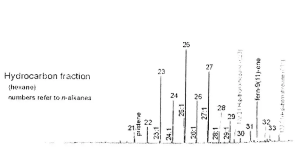
25

Hydrocarbon fraction

thexano)

4-numbers refer to n-alkanes 24 26 Z

29".

22

4732~

Figure 3-7: The is the hydrocarbon fraction of the sediment total lipid extract. Num-bers correspond with n-alkanes.

Figure 3-8: Gas chromatogram of hydrocarbon fraction from the saponified total lipid extract of the sediment of El Junco (15 cm depth). (Source: Smittenberg, unpublished. 2004.)

alcohol fraction

(20% ethyl acoteto in hoxsno) t'

numbs eer to n 0a2kar0 2s

Figure 3-9: Gas chromatogram of alcohol fraction from the saponified total lipid extract of the sediment of El Junco (15 cm depth). Numbers correspond with n-alkanols. Letters designate sterols. (Source: Smittenberg, unpublished. 2004.)

Chapter 4

Discussion

The first step in identification of candidates for D/H biomarker analysis is establish-ing distinctions between aquatic and terrestrial plant lipid inputs, as well as plant and non-plant inputs. Aquatic plant lipids will reflect the historical water balance of the lake, while terrestrial plant lipids will reflect the background D/H ratio produced by historical precipitation and cloud condensation. A comparison of lipid

distribu-tions in samples of prevalent plant species inputs with those in the sediment and the implications of these distributions follows. The goal of this comparison is to elucidate the origin of various components of the sediment TLE.

4.1

Fernene:

An Indicator for Terrestrial Plant Input

A photograph of the El Junco crater lake published in Nature in 1968 shows the

crater walls surrounding the lake crowded with the tree fern Cyathea weatherbyana

(F) [6]. The lipid analysis of the leaves of this fern show a great abundance of the

triterpenoidal hydrocarbon, fern-9(11)-ene. The sediment shows an abundance of the same compound in its hydrocarbon fraction. Fernene has only been isolated in terrestrial ferns and other closely related species [18]. Fern-9(11)-ene was not detected in the floating water fern, A. microphylla or the gully fern, T. Krausii. Its

detection in sea sediments has led some researchers to purport microbiota are also a source of fernenes [21]. However, no biogenic source has been found to support this. As such, fernenes in sea sediments could be transported by aerosols in a similar way as long-chain n-alkanes. It appears reasonable, in the case of the El Junco catchment, to assume that C. weatherbyana (F) is the source of fernene sedimentary input and thereby that terrestrial plant make some significant contributions to the lipid distribution preserved in the sediment record.

4.2

Observations on Fatty Acid Distributions

The most complete data set for any of the chemical classes is that for the fatty acids. Their abundance made peaks easy to identify and quantify. As such the informa-tion that can be gleaned from fatty acids is probably the most accurate informainforma-tion provided in this study. In this section, we discuss sources of high C16 and Cis fatty acid concentrations in samples, the viability of palmitic acid as a biomarker, and the potential reasons for disparities in the fatty acids distributions of plant and sediment data.

4.2.1

C

and C

Fatty Acid Abundances

High or variable content of saturated C16 and C18 fatty acids in some previous analy-ses of vascular plant samples has been attributed to bacterial contamination of sam-ples [3]. Bacterial compounds are known to contain high concentrations of these saturated fatty acids and as such, this seems to be a reasonable explanation for unex-pectedly high concentrations of these compounds in lipid extracts. The comparison of TLE and Rinse chromatograms from the twelve plant species tested here, however, indicates that the palmitic and stearic acids originate from the plant sample and not contaminants. Figure 4.2.1 shows the TLE and rinse fraction chromatograms for C. weatherbyana (F). The TLE shows the highest measured concentration of palmitic acid in any of the samples and moderately high levels of glue contamination. The rinse fraction shows very high levels of glue contamination (as would be expected

from any contaminant) and very low levels of C1 6 and C18. Other samples show a

similar pattern. Samples with very high glue or paper contamination show nearly imperceptible abundances of fatty acids the in rinse fraction. Samples with very low levels of paper and glue contamination show the highest relative abundances of fatty acids in the rinse fraction. Qualitatively, aquatic plants appear to show slightly higher rinse fraction abundances of unsaturated C1 6 and CIs fatty acids, indicating a

possible bacterial component. Regardless it is clear that both aquatic and terrestrial plants, and not their contaminants, produce significant amounts of these saturated fatty acids.

C C

0

2 Cyathea weatherbyana (F)

Total Lipid Extract

5 glue 15 20 25 30 35 40 45 50 55 min Cyathea weatherbyana (F) DCM Rinse glue 2 56 15 20 25 30 35 40 45 50 55 min

Figure 4-1: A comparison of lipid abundances in TLE and rinse fractions for C.

weatherbyana, the sample with the highest concentration of palmitic acid. Numbers