An alloy selection and processing framework for nanocrystalline materials

An alloy selection and processing framework for nanocrystalline

materials

SUBMITTED TO THE DEPARTMENT OF MATERIALS SCIENCE AND ENGINEERING IN PARTIAL FULFILLMENT OF THE REQUIREMENTS OF THE DEGREE OF

Doctor in Philosophy in Materials Science and Engineering at the

MASSACHUSETTS INSTITUTE OF TECHNOLOGY September 2018

© 2018 Massachusetts Institute of Technology. All rights reserved.

Signature of Author: ……… Department of Materials Science and Engineering

March 22, 2018

Certified by: ……… Christopher A. Schuh Danae and Vasilios Salapatas Professor of Metallurgy Thesis Supervisor

Accepted by: ………. Donald Sadoway Chair, Departmental Committee for Graduate Studies

An alloy selection and processing framework for nanocrystalline

materials

by

Arvind R. Kalidindi

Submitted to the Department of Materials Science and Engineering on March 22, 2018 in Partial Fulfillment of the Requirements for the Degree of Doctor of Philosophy in Materials Science and Engineering

ABSTRACT

Nanocrystalline materials have a unique set of properties due to their nanometer-scale grain size. To harness these properties, grain growth in these materials needs to be suppressed, particularly in order to process bulk nanocrystalline components and to use them reliably. Alloying the material with the right elements has the potential to produce remarkably stable nanocrystalline states, particularly if the nanocrystalline state is thermodynamically stable against grain growth. This thesis builds upon previous models for selecting alloy combinations that lead to thermodynamic stability against grain growth, by developing frameworks that extend to negative enthalpy of mixing systems and ordered grain boundary complexions. These models are used to develop a generalized stability criterion based on bulk thermodynamic parameters, which can be used to select alloy systems that are formally stable against grain growth. A robust statistical mechanics framework is developed for reliable thermodynamic observations using Monte Carlo simulations to produce free energy diagrams and phase diagrams for stable nanocrystalline alloys.

Thesis Supervisor: Christopher A. Schuh

ACKNOWLEDGEMENTS

The research presented in this work would not have been possible without the support of several colleagues, advisors, friends, and family.

When I started in the Schuh Group, I was new to the study of metallurgy. I want to thank Tongjai Chookajorn, Michael Gibson, and Zachary Cordero for taking me under their wing and bringing me up to speed on the thermodynamics and metals processing that led to the developments in this thesis. I also want to thank many other members of the Schuh Group – Oliver, Kathleen, Alan, Ting-Yun, Mostafa, Kathrin, Dor, Peter, Wenting, Eddie, Isabel, Ashley, Kat, Thomas, and others – for being supportive and helpful throughout my Ph.D. You have all had a great impact on this work and my wonderful time at MIT; it has truly been an honor and a privilege being your groupmate!

My advisor, Chris Schuh, provided constant guidance, inspiration, and wisdom throughout my Ph.D. When I joined the materials science department, I chose the Schuh Group because I believed Chris was an exceptional advisor and a brilliant researcher – looking back this was one of the best decision I have made in my life. Thank you Chris for helping me become the person I am today and for giving me the environment to thrive as a researcher over the past 5 years.

I want to thank Profs. Carl Thompson and Ju Li for advising me on the direction of this thesis as part of my thesis committee, and for lively discussions on grain boundaries and complexions that always gave me ample ideas to work on. I also want to thank Aslan Ahadi for collaborating on NiTi-W nanocrystalline alloys. My Ph.D. experience was made possible by the National Science Foundation Graduate Research Fellowship and the National Defense Science and Engineering Graduate Fellowship.

My time at MIT was marked by great friendship. To my roommates, Alex and Frank, our time at 45 Union St. was incredibly fun and enriching, and will be some of my fondest memories from MIT. Abigail, Ross, and Yang Yang, thank you for always being there when I wanted some company over soup dumplings, and Olivia, Seth, Jeremy, Brendan, Kate, and Jane, I will miss our Cambridge adventures and game nights. Neha, through the final year of my Ph.D. you have been an incredible new part of my life and have revealed in me an entirely new part of myself; I love you and am excited for our next steps together. My parents, Manju and Surya, and my brother, Bharath – your enduring love and support is the reason that I am who I am today and why I could even imagine embarking on this Ph.D. at MIT. Mom and Dad, thank you for giving me the confidence in my abilities and investing in my education to make all of this possible. Bharath, you will always be my better half and I will never enjoy anything more than watching sports with you at home eating chicken curry. And to my broader family, Mrudu, Anil, Meghana, Sanjana, Phani, Kiran, Sudeep, Anish, Pedda, Jayanthi, Siddhardth, Meera, Tattaya and Ammamma, I am incredibly grateful for having all of you be such big parts of my life and supporting me in everything I do.

Chapter 1: Introduction ...12

Section 1.1: What are nanocrystalline materials and why are they interesting? ...12

Section 1.2: Suppressing grain growth is the challenge to producing bulk nanocrystalline materials ....13

Section 1.3: Alloying to suppress grain growth in nanocrystalline materials ...15

Section 1.4: Existing frameworks for designing nanocrystalline materials ...17

Section 1.4.1: Analytical models for stability against grain growth and solute precipitation ...17

Section 1.4.2: Defining the configuration space of nanocrystalline alloys for improved thermodynamic models ...23

Section 1.4.3: Introduction to Monte Carlo simulations of alloy statistical mechanics ...25

Section 1.4.4: Monte Carlo simulations for designing nanocrystalline materials ...26

Section 1.4.5: Challenges of existing models for selection and processing of nanocrystalline materials to be addressed in this thesis ...33

Section 1.5: Outline of the main contributions of this thesis ...34

Chapter 2: Generalized stability criterion for stable nanocrystalline alloys ...36

Section 2.1: An analytical stability criterion for nanocrystalline alloys ...36

Section 2.1.1: Formulation of the stability criterion ...36

Section 2.1.2: Maps for selecting alloys to form stable nanocrystalline states based on the stability criterion ...40

Section 2.2: Incorporating entropic effects into the stability criterion: devising a more general lattice Monte Carlo simulation for nanocrystalline alloys ...43

Section 2.2.1: The compound unit approach for incorporating known equilibrium ordered states into the energy space of a lattice model ...44

Section 2.2.2: Defining the energetic parameters in the lattice model in terms of known alloy thermodynamic quantities ...50

Section 2.3: Comparison of the analytical model with Monte Carlo simulations ...53

Section 2.3.1: The effect of ∆𝐻𝑠𝑒𝑔 on the equilibrium nanostructure ...54

Section 2.3.2: The effect of ∆𝐻𝑠𝑒𝑔 on the equilibrium nanostructure ...58

Section 2.4. Guidelines for nanocrystalline alloy selection ...59

Chapter 3: Thermodynamics of Ni-Ti-W Nanocrystalline Alloys: A Case Study ...62

Section 3.1: Background and experimental analysis ...62

Section 3.1.1: Summary of experimental findings ...63

Section 3.2: Constructing the Monte Carlo simulation of Ni-Ti-W ...66

Section 3.3: Thermodynamic analysis of stability against grain growth in Ni-Ti-W thin films ...68

Section 3.4: Conclusions ...72

Chapter 4: Developing Phase Diagrams of Nanocrystalline Alloys ...73

Section 4.2: A new method for identifying thermodynamic equilibrium considering nanocrystalline

states ...76

Section 4.2.1: Model formulation of the Nanocrystalline Ising model ...76

Section 4.2.2: Defining 0 K ground states configurations in lattice models ...80

Section 4.3: Case study in developing free energy and phase diagrams for W-Ti ...81

Section 4.3.1: Order-disorder transitions at fixed grain boundary area ...81

Section 4.3.2: Order-disorder transitions for stable nanocrystalline states ...85

Section 4.3.3: Free energy and phase diagrams for stable nanocrystalline states ...89

Section 4.4: Exploration of a more efficient method for sampling the grain topology space ...94

Section 4.5: Conclusions ...98

Chapter 5: Pathways for Grain Refinement in Alloys with Nanocrystalline Ground States ...99

Chapter 6: Conclusions ...105

List of Figures

Figure 1: An example of the Hall-Petch relationship as observed through tensile and/or compression tests in vanadium, where the yield strength increases with decreasing grain size. This trend has been observed for several material systems, many of which are outlined in a review paper by Cordero et. al. from which this figure is reproduced with permission [7]. ...12 Figure 2: Rapid grain growth occurs at relatively low homologous temperatures in unalloyed

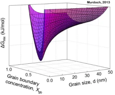
nanocrystalline materials (Reproduced from the thesis of Heather Murdoch [11]). ...14 Figure 3: This figure shows the free energy of a nanocrystalline alloy (with a large enough enthalpy of segregation to be thermodynamically stable) as a function of grain size. The minimum in free energy occurs at a finite, nanocrystalline grain size from which there is no driving force for grain growth

(Reproduced with permission from [27]). ...17 Figure 4: Diffraction patterns for Fe-Cu during annealing (heating at 20 K/min). Grain growth out of the nanocrystalline regime is observed following a phase transformation (white dots) in the Fe-Cu alloy (reproduced with permission from [38]). ...18 Figure 5: The free energy landscape of a stable nanocrystalline alloy as calculated by the regular

nanocrystalline solution model, where a minimum in free energy exists at a finite grain size in the

nanocrystalline regime (Reproduced with permission from [41]). ...20 Figure 6: The free energy diagram schematic for a binary alloy with the inclusion of nanocrystalline free energy curves (blue curve, which would be calculated from the RNS model). If the nanocrystalline free energy curve lies below the miscibility gap, the nanocrystalline state is formally stable against grain growth, but if it falls in the yellow, metastable, region it is unstable against forming a second phase (Reproduced with permission from [41]). ...20 Figure 7: Alloy selection map for W-based alloys produced using the RNS model based on enthalpies of mixing and grain boundary segregation for binary W alloys. On the right are free energy diagrams for two such binary alloys that show how the distinction between stable and unstable alloy systems were made by comparing the nanocrystalline free energy to the bulk miscibility gap. (Reproduced with permission from [46]). ...22 Figure 8: Phase diagram of Fe-Zr including the consideration of nanocrystalline states using the

CALPHAD method. This diagram shows the metastable nanocrystalline states using blue dashed lines (reproduced from [47] with permission). ...22 Figure 9: Schematic of the multi-scale considerations of nanocrystalline states in describing the

thermodynamic configuration (or phase) space (images are from the work of Millett et al. [50],

reproduced with permission of the publisher). ...24 Figure 10: An assessment of the thermodynamic stability of nanocrystalline Ni-W using an atomistic Monte Carlo simulation, where internal energies of nanocrystalline systems with grain sizes of 2, 3, and 4 nm are compared to a single crystalline (black line) system. Reproduced with permission of the publisher from [65]. ...28 Figure 11: A schematic of the lattice-based nanocrystalline alloy model developed by Chookajorn and Schuh [68], where each lattice site contains chemical and grain allegiance information. The configuration space of this model can explore topological degrees of freedom for the grain boundary network, enabling a more direct method for analyzing thermodynamic stability of nanocrystalline alloys. ...29

Figure 12: (a) Stability map of six general regions of nanocrystalline stability identified using the lattice-based Monte Carlo simulation: (b) bulk, single crystalline alloy with positive enthalpy of mixing, (c) phase separated polycrystal with undoped grain boundaries, (d) duplex nanostructured states with segregated grain boundaries, (e) segregated nanocrystalline state with positive enthalpy of mixing, (f) bulk. single crystalline alloy with negative enthalpy of mixing, (g) segregated nanocrystalline state with negative enthalpy of mixing. ...31 Figure 13: Pictorial representations of phase diagrams for a duplex nanocrystalline alloy constructed through Monte Carlo simulations at different compositions and temperatures first (a) without allowing for nanocrystalline states and (b) then allowing for nanocrystalline states in the configuration space

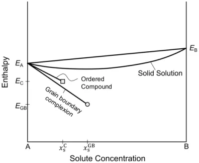
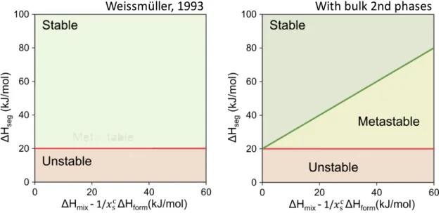
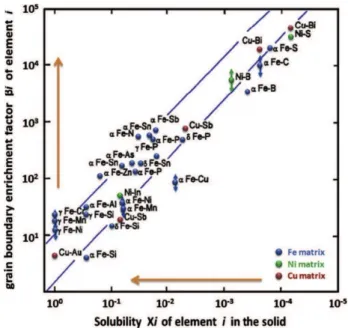
considered (Reproduced with permission from [72]). ...32 Figure 14: Schematic of the binary alloy energy diagram including an ordered phase (square) and a 2D grain boundary compound/complexion (circle) where the energy of non-stoichiometric compositions is calculated by the lever rule (lines). ...36 Figure 15: A stability map for selecting nanocrystalline alloys based on the bulk thermodynamic

parameters of the alloy pair (only enthalpic considerations of stability). On the left is the map produced by the Weissmüller criterion where the only configurations considered are the grain boundary segregated nanocrystalline state and a bulk solid solution. On the right is the map produced by the criterion derived in Section 2.1.1 where two phase states are also incorporated in the phase space considered. ...41 Figure 16: The experimentally-observed relationship between the terminal solubility of an alloy (which is related to the tendency for second phase formation) and the enrichment factor of the grain boundary (which is related to the enthalpy of grain boundary segregation). Reproduced with permissions from publisher [81]. ...42 Figure 17: Transition metal – transition metal binary alloys plotted using Miedema estimates [31,79] of ∆𝐻𝑚𝑖𝑥 and ∆𝐻𝑠𝑒𝑔 and density functional theory calculations of ∆𝐻𝑓𝑜𝑟𝑚 for compounds (attained from the Open Quantum Materials Database [74]) to observe the strength of correlation between the two axes of the stability map for physical alloy pairs. The solid line corresponds to perfect correlation between the axes, and the dashed line represents the stability criterion. ...43 Figure 18. (a) A possible definition of a compound unit for the ordered compound pictured in (b) where dark atoms are solute. (b) In addition to showing the equilibrium compound, the shading in this image shows a schematic of how the energy of an atom is calculated in the compound unit model, where darker atoms have a larger compound unit contribution to their energy. ...45 Figure 19: (a) A schematic of the compound superstructure for D03 and B2 compounds in body-centered

cubic binary alloys, with numbers signifying different interpenetrating FCC sublattices. Convenient compound units for D03 and B2 are shown in (b), with solute in black. Shaded atoms in (a) illustrate the

compound unit within the superstructure. ...47 Figure 20. Equilibrium states computed at 0 K via a Monte Carlo simulation under (a) the pairwise model and (b) the compound unit model. Only solute atoms are shown in the image, on a single (100) plane of the simulation cell. ...48 Figure 21. Equilibrium states as temperature is increased from 200 to 800 K at compositions of 10 and 25 at.%. Only solute atoms are shown in the image, with atoms ...49 Figure 22. Phase diagrams in (a) the pairwise model and (b) the compound unit model calculated via Monte Carlo. Phase transitions are denoted with solid lines, and two-phase regions are shaded. ...50

Figure 23: a) Schematic of ordering at a fixed grain boundary in the lattice model for a BCC lattice (blue – solute). b) Verification of Eq. 18 for calculating pairwise bond energies for the lattice model from a known enthalpy of segregation and a known grain boundary compound. ...52 Figure 24: Stability map based on Eqs. 15 and 16, when 𝑘𝛾 = 20 kJ/mol. Blue dots correspond to the ∆𝐻𝑠𝑒𝑔 series and the red squares correspond to the ∆𝐻𝑚𝑖𝑥 series for which equilibrium nanostructures are shown in Figs. 24 and 26, respectively. ...54 Figure 25. Equilibrium states of the ∆𝐻𝑠𝑒𝑔 series with a stable D03 compound (on left) and systems

without any stable compound (on right). Different grains have different shades of gray. Solute atoms are in blue if they are part of a D03 precipitate and red otherwise. ...56

Figure 26. The enthalpy relative to the bulk equilibrium state with increasing enthalpy of segregation for alloy systems with a stable D03 compound and without any stable compound. ...57

Figure 27. Equilibrium states of the ∆𝐻𝑚𝑖𝑥 series with a stable D03 compound (bottom) and without any

stable compound (top). Different grains have different shades of gray. Solute atoms are in blue if they are part of a D03 precipitate and red otherwise. ...58

Figure 28. Effect on the excess enthalpy of the grain boundary segregated state, upon varying the enthalpy of grain boundary segregation and the enthalpy of mixing independently. ...59 Figure 29: Transmission electron microscope (TEM) microstructures and corresponding SAEDs after annealing at 700 °C for 2 hours showing the effect of W addition on the grain growth behavior of (a) Ni50.9Ti49.1, (b) Ni50.3Ti48.8W0.8, (c) Ni52.4Ti39.7W7.9, and (d) Ni49.4Ti37.7W12.9 films. ...63

Figure 30: Variation of NiTi grain size with temperature measured with XRD (Scherer equation).

Annealing was done for 2 hours at each temperature. ...64 Figure 31: In-situ TEM images of the Ni49.4Ti37.7W12.9 thin film in the (a) as-deposited amorphous state,

and after annealing (b) to 1000 °C, (c) at 1100 °C for 1 min, (d) at 1100 °C for 4 min, (e) at 1200 °C for 10 sec, (f) and at 1200 °C for 70 sec. ...65 Figure 32: Thermal stability analysis of the Ni49.4Ti37.7W12.9 thin film, showing (a) a nanocrystal with size

of about 50 nm stable at 1200 °C with clear grain boundary segregation and W-rich precipitates, (b) an HRTEM image of the squared area in (a) showing a thick, amorphous grain boundary with a thickness of ~ 3 nm at 1200 °C, (c) room temperature HAADF-STEM image of the amorphous region showing Ni segregation at the grain boundary, and (d) two typical room temperature EDX compositional line scans across the grain boundary complexions showing both Ni and W segregation. ...65 Figure 34: Thermodynamic analysis of grain boundary segregation in the NiTi-W alloy system, with (a) the concentration of solute at the grain boundary at 600 °C and (b) the grain boundary enrichment of solute at the grain boundary at 600 °C, and (c) the grain boundary enrichment of W at 600 °C and 1200 °C. Dashed lines at enrichment factors of 1 are used to visually compare (b) and (c). ...69 Figure 35: Monte Carlo simulation of the Fe-Cu system conducted by Clark et. al. where the equilibrium predicted by the simulation is not the thermodynamic equilibrium state. (Reproduced with permission from the publisher [99]). ...73 Figure 36: On the left for each simulation is the equilibrated system where solute are in black and colors denote the grain numbers of the solvent. On the right, the grain numbers of the solute are shown in color. In both cases, the grain numbers of the solute are random, where solute are maximizing their coordination of grain boundary solute-solvent bonds. This leads to unphysical ground states that complicates the development of a robust Monte Carlo simulation. ...75

Figure 37: Schematic representation of the framework for identifying free energy minimizing

nanocrystalline states by separately exploring solute and grain boundary network configuration spaces. The four configurations shown are all of the same volume (area), but have different relative proportions of grain boundary area (length); comparing across them at constant composition therefore speaks to the energetics of the boundary area and its interaction with the solute. ...77 Figure 38: All minimizing configurations for a 2D hexagonal lattice with 28 solute atoms, with

complexions with a preference for A-B grain boundary bonds and B-B grain boundary bonds placed in separate rows. Solvent and solute atoms are colored gray and blue respectively. †Wetting complexions form a continuum as the precipitate can intersect the grain boundary in several ways; as such, we have not given them different names. ...81 Figure 39: Order-disorder transitions of 1 at.% alloys at fixed grain boundary volume fraction for each of the four cases. Heat capacities are presented in the first row, followed by crystalline and grain boundary order parameters in the second row, and total system energy in the form of entropic energy, internal energy, and free energy in the third row. ...82 Figure 40. (a) Heat capacities from 0 to 2000 K for 1 at.% alloys with fixed grain boundary volume fraction in the saturated, oversaturated, and single crystal regime, and (b) the corresponding entropies and (c) free energies. ...84 Figure 41. (a) Free energy as a function of grain boundary volume fraction at three temperatures: 0 K, 600 K where the stable grain boundary volume fraction is lower, 840 K where the solid solution phase first becomes stable, and 2000 K. (b) The same free energies are also shown with respect to grain size. ...85 Figure 42: Order-disorder transitions for a 1 at.% stable nanocrystalline alloy. (a) The free energy,

entropic energy, and internal energy, accompanied by (b) the grain boundary and crystalline order parameters, and (c) the grain boundary volume fraction are shown as a function of temperature from 0 K to 2000 K...88 Figure 43: The equilibrium microstructures at 300 K, 500 K, 700 K, and 900 K. ...88 Figure 44: The free energy diagram at 1100 K, 1550 K, and 2000 K for solute concentrations from 1-10 at.%, where the solid lines represent systems where the solid solution is stable and the dashed lines represent systems with stable grain boundaries in equilibrium with a solid solution. ...90 Figure 45: (a) The phase diagram for a stable nanocrystalline alloy, where the solid line and black dots represent the transition temperature for forming a solid solution from the nanocrystalline state

(nanocrystal solvus). The blue squares represent the transition temperature for forming a solid solution from a bulk precipitate, which form the single crystal solvus for when nanocrystalline states are not considered. The white region is a two-phase region. (b) The equilibrium microstructure for a 4 at.% alloy at 1000° C (denoted by a star in (a) ) for which the concentration of solute in the crystalline region is that of the nanocrystal solvus when read from the phase diagram according to the lever rule. ...92 Figure 46: The phase diagram with curves of constant grain size (dashed lines) where red markers denote the temperature at which a particular grain size is stable for a given concentration. ...93 Figure 47: A weighted voronoi tessellation where black dots represent nodes used to generate the

structure and different grains are colored differently. ...96 Figure 48: 0 K equilibrium microstructures as calculated by the Monte Carlo simulation. The ΔHmix is 20

kJ/mol and the ΔHseg is listed above each simulation. Systems above ΔHseg = 40 kJ/mol are expected to

satisfy the stability criterion. Different colors represent grains, black dots are solute. Grain boundary segregation is observed in all states with grain boundaries. ...96

Figure 49: 1500 K equilibrium microstructures as calculated by the Monte Carlo simulation. ...97 Figure 50: For grain sizes smaller than the equilibrium grain size, there is a driving force for grain growth. For grain sizes larger than the equilibrium size, the direction of the free energy gradient leads to a driving force for grain shrinkage instead of grain growth. ...100 Figure 51: The driving force for grain growth is to decrease the grain boundary area (i.e. eliminate the excess energy due to defects). The driving force for grain shrinkage is to increase the amount of solute that is in a grain boundary segregated state, denoted as ΔEchem. ...100

Figure 52: (Top) A schematic showing how nucleation of a grain at a triple junction could occur as the reverse of a grain growth process. (Bottom) A schematic of the solute distribution during nucleation of such a grain. ...102 Figure 53: (Top) A schematic of how grain boundaries evolve in response to curvature in a case of grain shrinkage versus grain growth. The energetics of grain shrinkage from a flat surface in the lattice model were studied using a sinusoidal perturbation (pictured in (a)). The energy of the system decreases

List of Tables

Table 1. Predicted stability classification according to Eqs. 15 and 16 for alloy systems for which the thermal stability has been experimentally studied. ∆𝐻𝑠𝑒𝑔 critical is the enthalpy of grain boundary segregation needed for the alloy system to be stable. If the enthalpy of grain boundary segregation is within 5 kJ/mol of satisfying or failing either criteria, both likely classifications are specified. ...60 Table 2: Thermodynamic parameters for the Ni-Ti-W systems used for the Monte Carlo simulations. ....67

Chapter 1: Introduction

Section 1.1: What are nanocrystalline materials and why are they interesting?

Most structural materials used commercially are polycrystalline, meaning that they contain several crystalline regions, called grains, which each have different lattice orientations. At the intersection of grains, there is a planar defect due to the misorientiation of the two adjoining lattices, called a grain boundary. Structural materials produced through conventional processing methods, e.g. casting or sintering, typically have grain sizes in the 10s of microns and up to millimeter length scales. On the other hand, polycrystalline materials prepared through thin film fabrication methods, such as sputtering or electrodeposition, generally have grain sizes that are orders of magnitude smaller, and can be as small as a few nanometers [1-3].

These materials, when possessing grain sizes less than 100 nm, are referred to as nanocrystalline materials. The structural properties of these nanocrystalline materials have been studied in thin film form quite extensively. Most notably, nanocrystalline materials have a high yield strength, as described by the Hall-Petch relationship (Figure 1) [4-7], an empirical observation that the yield strength, σy, increases with decreasing grain size, d, as 𝜎/ = 𝜎1+ 𝑘 3₄,

where k and σ0 are material-specific constants.

Figure 1: An example of the Hall-Petch relationship as observed through tensile and/or compression tests in vanadium, where the yield strength increases with decreasing grain size.

The high yield strength of nanocrystalline materials has several promising applications. For instance, in material applications where plastic deformation constitutes failure, one can use a fraction for the same material to meet load tolerances if the material is nanocrystalline. As a result, producing nanocrystalline materials can enable light-weighting in structural applications such as automobiles and aircrafts. Additionally, certain applications, such as tooling or coatings, are limited by the yield strength of the material. Today, W-carbide and diamond films are often used in these applications where the material hardness is critical to performance. Refining the grain structure can enable alternate pathways to producing material hardness that rivals and potentially surpasses that of current high-hardness materials. This has the potential to decrease costs, increase material performance, and offer more diversity in materials for high hardness applications, which can decrease reliance on rare or hazardous materials (such as depleted uranium or chromium [8, 9]).

Section 1.2: Suppressing grain growth is the challenge to producing bulk nanocrystalline materials

Grain sizes in the nanocrystalline regime can be readily formed in thin films. However, producing a bulk part that is nanocrystalline is a serious challenge, due to the propensity of nanocrystalline materials to undergo grain growth at low homologous temperatures. Nanocrystalline materials have a much higher density of grain boundaries, which carry an excess energy (~ 1 J/m2_{) as defects [10], than a courser grained material. Due to the high density of grain}

boundaries, the driving force for grain growth is substantially higher for nanocrystalline materials compared to course grained materials: doubling the grain size of a nanocrystalline material leads to a ~1000 times larger decrease in grain boundary area than does doubling a micron-scale grain size.

As a result, nanocrystalline materials undergo rapid grain growth at relatively low temperatures (Figure 2) [11]. For instance, nanocrystalline Ni undergoes grain growth from grain sizes in 10s of nanometers to 100s of nanometers in just 30 minutes at 300 °C [11]. The use of conventional routes for producing bulk parts generally require time at elevated temperatures. Solidifying into the nanocrystalline regime from a liquid phase requires a high nucleation rate and a low coarsening and growth rate, conditions that either require unreasonable cooling rates, or in

glass-formers require avoiding glass transitions. Alternatively, one can produce nanocrystalline materials from bulk metallic glasses, but producing bulk metallic glasses is in itself a challenge and such devitrified materials can be brittle due to a strong tendency to form intermetallics [12]. Powder-route processing by sintering nanocrystalline powders into a bulk part requires avoiding substantial grain growth at sintering temperatures.

Figure 2: Rapid grain growth occurs at relatively low homologous temperatures in unalloyed nanocrystalline materials (Reproduced from the thesis of Heather Murdoch [11]).

The key challenge to producing bulk nanocrystalline materials is therefore to mitigate grain growth at elevated temperatures. Grain growth is enabled by grain boundary motion, the speed (v) of which can be described by:

𝑣 = 𝑀𝛾𝜅 (1)

where M is the mobility of the grain boundary (and is expected to have an Arrhenius behavior), γ is the grain boundary energy (decreases linearly with temperature), and κ is the curvature of the grain boundary (high in bulk nanocrystalline materials) [13]. Therefore, to avoid substantial grain growth at low temperatures in nanocrystalline materials, either the mobility needs to be drastically reduced so that grain boundaries cannot move easily or the excess energy of the grain boundary itself needs to be reduced so that grain boundaries have a smaller driving force to move and cause

Section 1.3: Alloying to suppress grain growth in nanocrystalline materials

Alloying is a powerful way to reduce grain growth as it can both reduce the grain boundary mobility and decrease the grain boundary energy. Grain boundary mobility is decreased by two different mechanisms in alloys. In multiphase alloys, precipitates of secondary phases can pin grain boundaries [14,15], known as Zener pinning, providing an obstacle which grain boundaries must pass through, thereby increasing the activation energy for grain boundary motion. To stabilize nanocrystalline alloys against grain growth through Zener pinning, the precipitate size must be nanometer scaled as well [14,15]. This poses a secondary challenge in preventing coarsening of fine precipitates, particularly since these precipitates reside on grain boundaries which can act as fast diffusion pathways for coarsening. As a result, second phases such as oxides and carbides that are more likely to be interface-limited in coarsening are generally required for Zener pinning to be successful in nanocrystalline materials [16,17]. Grain boundary mobility can also be decreased by solute drag, where solute species in solid solution provide resistance to grain boundary motion as the grain boundary must incorporate the solute into its free volume and then reject the solute as it passes by [18-20]. This mechanism similarly can increase the activation energy for grain boundary motion.

Suppressing grain boundary motion is referred to as a “kinetic” route to stabilizing nanocrystalline materials against grain growth at elevated temperatures [21]. Due to the Arrhenius relationships underlying these kinetic mechanisms, increasing the activation energy by a factor, X, allows the alloy to be stable against grain growth up to temperatures of roughly a factor of X higher than for the pure solvent material. While such increases in the temperature at which grain growth occurs has the potential to enable the processing of bulk nanocrystalline alloys, identifying the right alloying elements is complicated by the difficulty in assessing activation energies of grain boundary motion in alloys [22]. Thus, even though these mechanisms are well-established, they have not yet enabled the systematic development of bulk nanocrystalline alloys.

Alloying can also decrease the grain boundary energy when alloying elements segregate to the grain boundary, decreasing the driving force for grain growth [23-25]. Grain boundary segregation is the presence of an excess concentration of solutes in the grain boundary with respect to the bulk concentration of that solute element. The magnitude of the decrease in energy at the grain boundary is measured by the enthalpy of grain boundary segregation for an alloy system.

The enthalpy of grain boundary segregation is defined as the change in energy between a random distribution of solutes in the system and the equilibrium, grain boundary segregated state on a per mole basis.

Designing alloys based on the grain boundary segregation effect as a means to suppress grain boundary motion is referred to as a “thermodynamic” route to stabilizing nanocrystalline materials [21]. The enthalpy of segregation decreases the grain boundary energy linear manner, and so this effect is generally weaker than the kinetic drag and pinning effects which have exponential effects on grain boundary motion. However, unlike the kinetic route, the thermodynamic route has the potential to produce a formally stable nanocrystalline state.

The concept of a formally stable nanocrystalline alloy was first introduced by Weissmüller [26-27]. Using the Gibbs adsorption isotherm, Weissmüller showed that if the segregation of solute species is energetically favorable enough to offset the excess free energy associated with the grain boundary, then the segregated grain boundary states would be stable against grain growth. Using classical thermodynamics, Weissmüller derived an expression for the grain boundary energy, γ, for a dilute binary alloy with solute segregation at the grain boundaries:

𝛾 = 𝛾₁− 𝛤_:;< Δ𝐻_:>?+ 𝑅𝑇ln 𝑥_D (2)

In this expression, γ0 is the pure solvent grain boundary energy, which can be offset by an alloying

addition with a positive enthalpy of grain boundary segregation, ΔHseg, defined here as the enthalpy

required to take a single solute atom from the crystalline region and place it into the grain boundary in the dilute limit. Γsat is the specific solute excess at the solute-saturated grain boundary, and xc is

the solute concentration in the crystalline region. This equation shows that the grain boundary energy is decreased linearly with the enthalpy of grain boundary segregation. Based on this expression, Weissmüller showed that strongly segregating solute species can reduce the grain boundary energy to zero, or more specifically, can lead to a minimum in the free energy of the alloy with respect to grain boundary area, EF_EG = 0, at a finite grain size as shown in Figure 3. Such a nanocrystalline state in the alloy has no driving force to change its grain boundary area when the grain size is equal to the equilibrium grain size; the nanocrystalline state is stable against grain growth, because grain growth would require ejection of some solute into the grain interiors at an

Figure 3: This figure shows the free energy of a nanocrystalline alloy (with a large enough enthalpy of segregation to be thermodynamically stable) as a function of grain size. The

minimum in free energy occurs at a finite, nanocrystalline grain size from which there is no driving force for grain growth (Reproduced with permission from [27]).

Unlike the kinetic route, the enthalpy of grain boundary segregation can be estimated theoretically through density functional theory calculations, embedded atom-type potentials, as well as empirical Miedema models [27-31]. As a result, identifying alloy systems that are stable thermodynamically against grain growth is a more viable route to developing bulk nanocrystalline materials systematically. In the next section, previous models for identifying and developing such alloy systems are discussed, which form the foundation on which the frameworks in this thesis are developed.

Section 1.4: Existing frameworks for designing nanocrystalline materials

Section 1.4.1: Analytical models for stability against grain growth and solute precipitation

Early alloy systems developed using the Weissmüller framework were typically observed to exhibit stability of nanocrystalline grain sizes at low annealing temperatures. However, at the elevated tempreatures required for processing bulk nanocrystalline parts, these alloys were often observed to undergo rapid grain growth [32-38]. Experiments monitoring grain growth often

observed that second phases would form at the instance when rapid grain growth was initiated, an example of which is shown in the Fe-Cu system in Figure 4 [38].

Figure 4: Diffraction patterns for Fe-Cu during annealing (heating at 20 K/min). Grain growth out of the nanocrystalline regime is observed following a phase transformation (white

dots) in the Fe-Cu alloy (reproduced with permission from [38]).

This revealed a key limitation of the model developed by Weissmüller for thermodynamic stability of the nanocrystalline state: the assumption that the solutes are in dilute concentrations. Because the Weissmüller model does not account for the potential for solutes to form a second phase, it effectively only compares the free energy of the nanocrystalline state to that of a single crystal solid solution at the same concentration. To be truly stable, the nanocrystalline state needs to be energetically preferred to any single crystalline state, including those containing second phases.

To begin to alleviate the dilute limit assumption from Weissmüller’s model, Trelewicz and Schuh [39] used a regular solution approach to develop the regular nanocrystalline solution (RNS) model. In addition to a crystalline grain interior region, the RNS model includes a grain boundary region, defined by two variables. This first variable is the grain boundary volume fraction, which in their model mapped monotonically to grain size. The second variable is the grain boundary solute concentration, which is a measure of the degree of grain boundary segregation. As in the classical regular solution model, the free energy of the alloy state is determined from the internal energy, calculated by summing the energies of the bonds (assuming a random distribution of solute in the crystalline and grain boundary regions and considering nearest-neighbor pairwise

Rapid  Grain   Growth Fe-­Cu

interactions), and from the configurational entropy of the full system. A particular alloy system can be described by interaction parameters, ω, which are used to define the solute-solvent bond energies within the crystal (c) and grain boundary (gb) regions:

𝜔_D = 𝐸_KLD ₋  𝐸KKD + 𝐸LLD 2   (3)   𝜔_?O = 𝐸_KL?O −  𝐸KK ?O _{+ 𝐸} LL?O 2   (4)  

where E is the energy per bond classified by the subscript which represents the types of species bonded (A – solvent, and B – solute) and the superscript which denotes the bond type. The two interaction parameters can be related to the enthalpy of mixing and enthalpy of segregation to link model predictions of stability to actual alloys [39,40]:

𝛥𝐻_QRS = 𝑧𝜔_{U (5)}  

𝛥𝐻_VWX = 𝑧 𝜔_U−𝜔XY

2 −

1

2𝑧𝑡(𝛺^𝛾1^− 𝛺G𝛾1G (6)   where 𝛺 is the atomic volume of an element, z is the coordination number, and t is the thickness of the grain boundary.

The free energy calculated by the RNS model is not restricted to dilute solutions or saturated grain boundaries. The equilibrium state is the one that minimizes the free energy, but unlike in the Weissmüller model where the only degree of freedom is the grain size, in the RNS model both the grain size and the concentration at the grain boundary are equilibrium quantities. The free energy landscape for a particular alloy chemistry is shown in Figure 5 [41]. The Trelewicz-Schuh RNS model has also been refined and extended by other authors to different more specific situations, with similar general outputs in each case [42-45].

Figure 5: The free energy landscape of a stable nanocrystalline alloy as calculated by the regular nanocrystalline solution model, where a minimum in free energy exists at a finite grain

size in the nanocrystalline regime (Reproduced with permission from [41]).

Figure 6: The free energy diagram schematic for a binary alloy with the inclusion of nanocrystalline free energy curves (blue curve, which would be calculated from the RNS model). If the nanocrystalline free energy curve lies below the miscibility gap, the nanocrystalline state is formally stable against grain growth, but if it falls in the yellow, metastable, region it is unstable

against forming a second phase (Reproduced with permission from [41]).

Murdoch and Schuh used the RNS model to explicitly define metastability and stability of nanocrystalline alloys against grain growth [41]. In order for the nanocrystalline state to be stable,

equilibrium state on the free energy diagram. As shown in Figure 6, Murdoch and Schuh used a regular solution treatment for the bulk miscibility gap and defined a nanocrystalline state as stable if it lies below the miscibility gap.

This is an immensely valuable insight for the selection of alloying elements for stabilizing nanocrystalline alloys against grain growth, as it improves upon the largest shortcoming of the Weissmüller model by accounting for driving forces for forming second phases. As a result, nanocrystalline alloys that are found to be stable under this criterion would be expected to be formally stable against grain growth up to elevated temperatures and ideal candidates for producing bulk nanocrystalline materials. Through a series of simulations, Murdoch and Schuh found that the stability criterion can be written as:

∆𝐻_:>? > 𝑐 ∆𝐻_abc d ₍₇₎

where the coefficients a and c depend on the homologous temperature and were fitted to the results of the RNS model.

Chookajorn et al. [46] developed a stability map for W alloys using this analytical approach, shown in Figure 7 with corresponding free energy diagrams illustrating the difference between a predicted stable nanocrystalline alloy, W-Sc, and a classical bulk stable alloy, W-Ag. The map delineates the alloy pairs for which at least one nanocrystalline alloy has an energy lying below the miscibility gap free energy. This map was used to identify W-Ti as a candidate for exhibiting thermodynamic stability at 1100 °C. This system was subsequently explored with a W-20 at.% Ti alloy that exhibited no significant changes in grain size after annealing at 1100 °C for 1 week. The results of Chookajorn et al. [46] show that a simple analytical model such as the RNS model can be used to rapidly screen possible alloys that may exhibit nanocrystalline ground states.

The RNS framework also has the potential to guide the processing of nanocrystalline alloys by describing how the free energy landscape of nanocrystalline states is affected by processing parameters such as temperature and composition. Zhou and Luo [47] extended the approach of Murdoch and coworkers [41,46] by using a CALPHAD evaluation of free energies to produce a phase diagram for Fe-Zr alloys, shown in Figure 8. They included nanocrystalline states computed using a regular solution model for grain boundary segregation developed by Wynblatt and Chatain [23]. In this case, the segregated nanocrystalline states were less energetically favorable than the Fe23Zr6 compound, and thus only metastable grain size information could be provided. In an alloy

exhibiting true nanocrystalline stability, phase diagrams are expected to include phase transitions between bulk phases and nanostructured states, as well as two-phase regions possessing unique nanostructural features.

Figure 7: Alloy selection map for W-based alloys produced using the RNS model based on enthalpies of mixing and grain boundary segregation for binary W alloys. On the right are free

energy diagrams for two such binary alloys that show how the distinction between stable and unstable alloy systems were made by comparing the nanocrystalline free energy to the bulk

miscibility gap. (Reproduced with permission from [46]).

Figure 8: Phase diagram of Fe-Zr including the consideration of nanocrystalline states using the CALPHAD method. This diagram shows the metastable nanocrystalline states using blue dashed

While these analytical models have been useful to advancing the development of nanocrystalline alloys, they are limited by regular solution assumptions. In order for regular solution assumptions to be reasonably valid, the interaction parameters should be of relatively low magnitudes in order for there to be a random distribution of solute in a region. However, stable nanocrystalline states are formed due to a high tendency for grain boundary segregation, which means that they inherently possess large interaction parameters for solutes at the grain boundary.

In effect, the constraint of random distributions within the grains and at the grain boundaries of nanocrystalline states in the RNS model strongly limits the possible configurations of nanocrystalline states considered in these models [48]. Expanding the configuration space (or the phase space in statistical mechanics terms) considered in nanocrystalline alloys is critical to understand the thermodynamics of nanocrystalline alloys []. This larger configuration space is too complex to capture analytically, so we must build thermodynamic simulations.

Section 1.4.2: Defining the configuration space of nanocrystalline alloys for improved thermodynamic models

Before exploring the methods available to perform a thermodynamic exploration of the nanocrystalline alloy configuration space, let’s define what the configuration space for a nanocrystalline alloy is, and what reasonable simplifications can be made.

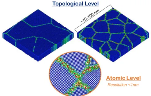
In bulk alloys, the configuration space to be considered in determining the equilibrium state can often be reduced to the distribution of chemical species on a lattice. However, to consider grain boundary segregation, the portion of the phase space surveyed for free energy minima must be expanded. This is a multi-scale challenge: grain boundaries are disordered regions of the lattice at the atomic scale and form a complex network throughout the system at the topological, meso-scale level, as illustrated in Figure 9. Details at these different scales are all important to a full assessment of equilibrium. At the topological level, the grain boundary network determines the equilibrium average grain size, the solute interaction with the grain boundaries, and whether nanocrystalline states are preferable to bulk phases. At the atomic-scale, the local positioning of atoms in the inhomogeneous environment of the grain boundary is important for capturing segregation phenomena accurately.

Figure 9: Schematic of the multi-scale considerations of nanocrystalline states in describing the thermodynamic configuration (or phase) space (images are from the work of Millett et al. [50],

reproduced with permission of the publisher).

A multi-scale description of the grain boundary state is difficult to capture analytically, and as such the analytical models discussed in the previous subsection rely on the definition of a single average grain boundary site, and the fraction of those sites in the system then becomes the core descriptor of a nanocrystalline structure. Atomistic simulations, on the other hand, have demonstrated great utility at both describing the atomistic environment of the grain boundaries of nanocrystalline states, as well as the grain topology in studies of grain growth. Taking advantage of this, Millett and coworkers performed molecular statics and molecular dynamics (MD) studies of stability against grain growth [50-52]. Using a Lennard-Jones potential, their simulations showed that placing sufficiently larger solute atoms at the grain boundaries successfully arrested grain growth by reducing the excess grain boundary energy to zero. However, from a thermodynamic perspective, there are two critical features missing from such an approach for studying nanocrystalline ground states. First, grain boundary segregation should occur thermodynamically, such that the chemical potential of the alloy is constant throughout the system, which is not obeyed by artificially placing solute at the grain boundary. Second, the simulation must be sufficiently long such that bulk phases can nucleate, which is not easy to capture in an

MD simulation due to the longer time-scales associated with diffusion. For the time and length scales required to study the thermodynamics of nanostructured states, a statistical mechanics-based approach offers many advantages, and it is to these models that we turn our attention.

Section 1.4.3: Introduction to Monte Carlo simulations of alloy statistical mechanics

In statistical mechanics, the equilibrium behavior of an alloy is determined by taking thermal averages at the atomic level. For closed systems at a fixed temperature (i.e. in the canonical ensemble), the probability that a particular alloy configuration, m, is the equilibrium state depends on the energy of the configuration, Em, as 𝑃_Q = eg

hi

jk /𝑄, where k is the Boltzmann constant,

and T is the absolute temperature. The partition function, 𝑄 =   _R𝑒gjkhn, represents the size of the

configuration space and can be related to thermodynamic quantities, such as entropy and free energy. Thus if the energies of all configurations are known, the canonical ensemble partition function and the probabilities of each configuration can be determined and used to identify the preferred state of the alloy and calculate relevant thermodynamic information.

Monte Carlo is a stochastic method for approximating the thermal averages of statistical mechanics, capturing statistical fluctuations and connecting this information to macroscopic thermodynamic quantities. Sampling the configuration space is not a trivial task, as most configurations in the space contribute insignificantly (have very low probabilities) to the equilibrium, and thus simple sampling methods can be prohibitively inefficient. Monte Carlo simulations can be devised to instead sample configurations in the phase space at a rate corresponding to their probability of occurring in the ensemble, which is termed importance sampling. This is done by sampling the space through transitions, where a new configuration, j, is considered for sampling by applying a transformation to the current configuration, i. The Metropolis algorithm [40] then provides stochastic rules for accepting the transition from state i to

j by the transition probabilities:

𝑃R→p =   e

gqr_stgqn_{, if  𝐸} p > 𝐸R

According to this method, if the new configuration has a lower energy, the system always transitions into it, but if it has a higher energy the transition only occurs with a probability determined by the energy increase and the temperature (with transitions to higher-energy states more probable at elevated temperatures). Typically, an initial configuration is chosen, and transitions are attempted and performed according to the Metropolis algorithm until the system reaches equilibrium, at which point any dependence on the choice of initial configuration has been eliminated. For more background on Monte Carlo simulations, I highly suggest reading [53].

When defining transitions, the goal is to efficiently explore the configuration space with respect to its degrees of freedom. For example, for bulk crystalline alloys the alloy configuration space can be simplified to consider the distribution of solute on a lattice, as is done in the Ising model [54]. In closed systems, atom swaps are used to transition through the configuration space, where a random solute atom and solvent atom from within the lattice have their lattice positions exchanged, leading to a new configuration. The nature of this transition has two important features. First, this mechanism is not meant to represent a physical process, but rather to sample the configuration space without getting trapped in metastable states corresponding to local minima in the free energy, which is assisted by the long-range nature of these swaps. At the same time, a single atom swap does not produce an independent sample configuration from the phase space; it is highly dependent on the previous configuration. Therefore, to collect uncorrelated samples of the phase space, and to satisfy the ergodic hypothesis, many swaps must be performed in between samples before including a new state in calculations of macroscopic thermodynamic quantities. At moderate temperatures, it has been demonstrated in a number of studies that this sampling approach successfully finds the global minimum in free energy and captures the expected phase equilibria as well as enthalpic and entropic behavior of binary alloys [55-58].

Section 1.4.4: Monte Carlo simulations for designing nanocrystalline materials

This general Monte Carlo formulism can be adapted to include grain boundaries in the description of the configurational space of the alloy. As discussed in Section 1.4.2, the presence of grain boundaries and their interaction with segregants introduces additional degrees of freedom at both the atomistic scale, related to the structure of the grain boundary, and at the meso-scale, related to the topology and crystallography of the grain boundary network. Two types of Monte

Carlo simulations have been developed, each designed to focus at a particular scale, and to provide a different level of information regarding the stability of nanocrystalline states.

Section 1.4.4.1 Monte Carlo Simulations at the Atomic Level of Grain Boundaries

A particular grain boundary can take on different equilibrium atomic configurations, known as complexions [59-60], with varying grain boundary thicknesses, disorder, and chemistry. As such, Monte Carlo studies of grain boundary segregation at the atomic level should consider the added positional degrees of freedom available for atoms at the grain boundary by including appropriate transition operations to reach the equilibrium grain boundary structures for a particular nanocrystalline alloy. Simulations to study grain boundary segregation in this way were first developed to measure the extent of segregation at different grain boundaries, and to analyze structural transitions that occur within the grain boundary [28,29,61-64]. Such methods have been more recently adapted by Detor and Schuh [65], and Purohit and coworkers [66,67] to study the thermodynamics of nanocrystalline alloys.

The transition event used to sample the phase space of the alloy must allow atoms to relax locally. A common approach is to accompany each solute-solvent atom swap with atomic relaxation of the system to maintain zero hydrostatic stress, for example by straining the system incrementally and using conjugate gradient relaxations to allow the atoms to utilize the off-lattice degrees of freedom at the grain boundary. The new, depressurized state is then considered for transition according to the Metropolis algorithm, where the energies of each state are typically calculated using many-body potentials. Such a simulation produces the lowest free energy state for the alloy, but is constrained to the initial grain topology provided, since the transition event does not create or remove grain boundary area, and the relaxations permitted do not allow for large atomic reconfiguration. Thus in order to assess nanocrystalline stability, simulations at fixed grain sizes must be compared to single crystal simulations to determine the more favorable state, as these states are not considered simultaneously in the Monte Carlo framework. Figure 10 shows the work of Detor and Schuh on Ni-W using this approach to understand the composition ranges in which the internal energy of the nanocrystalline states (considering systems with average grain sizes of 2, 3, and 4 nm) was lower than that of a single crystalline (the SC curve) system [65]. However, only the enthalpies are considered in such a calculation. Because the free energies are not known,

accurate assessment of thermodynamic stability at finite temperatures is difficult with this approach.

Figure 10: An assessment of the thermodynamic stability of nanocrystalline Ni-W using an atomistic Monte Carlo simulation, where internal energies of nanocrystalline systems with grain sizes of 2, 3, and 4 nm are compared to a single crystalline (black line) system. Reproduced with

permission of the publisher from [65].

Another shortcoming of atomistic Monte Carlo simulations for considering the stability of nanocrystalline states is that the portion of the phase space considered in a given simulation does not simultaneously include both nanocrystalline and single crystalline states. Therefore, to identify the stable nanocrystalline state, all possible nanocrystalline configurations at the topological level should be considered in the free energy minimization to identify the nanostructure of the equilibrated state. As a result, while the atomic position degrees of freedom at the grain boundary are important at the grain boundary structure level, the topological degrees of freedom of the grain boundary network should be explored as part of the Monte Carlo sample space in order to determine if a nanocrystalline state exists at equilibrium and to assess the meso-scale structure of the state.

Section 1.4.4.2 Monte Carlo Simulations at the Topological Level of Grain Boundaries

In order for a Monte Carlo simulation to provide information on the stability of nanocrystalline states, the sampling method should have the freedom to add or remove grain boundary area in search of the lowest free energy nanostructure. To make such a description of the configuration space more computationally feasible, it is convenient to start from a more

coarse-grained approach that foregoes the atomic level description of grain boundary structure and its dependence on local factors, such as the adjoining grain orientations, in favor of describing the effects of alloying on a larger network of average grain boundaries. Chookajorn and Schuh [68] modified the Ising approach to incorporate the possibility of stable nanocrystalline states. Unlike the original Ising model, each lattice site in the alloy is not only prescribed with an occupying chemical species, but is also associated with a particular grain, denoted by a grain number, such that nearest neighbor bonds between two lattice sites with different grain numbers constitute a grain boundary, as shown in Figure 11.

Figure 11: A schematic of the lattice-based nanocrystalline alloy model developed by Chookajorn and Schuh [68], where each lattice site contains chemical and grain allegiance information. The configuration space of this model can explore topological degrees of freedom

for the grain boundary network, enabling a more direct method for analyzing thermodynamic stability of nanocrystalline alloys.

Under this description, the internal energy of a particular configuration, Em, can be written

by summing nearest neighbor bonds, as was done in the RNS model:

Grain 1 Grain 2 Grain 3 Chemical Identity Grain Allegiance Crystalline  Bond Grain  Boundary   Bond

𝐸_Q = 𝑁_KKD _𝐸

KKD + 𝑁KLD 𝐸KLD + 𝑁LLD 𝐸LLD + 𝑁KK?O𝐸KK?O + 𝑁KL?O𝐸KL?O+ 𝑁LL?O𝐸LL?O (9)

where E is the pairwise bond energy between the species specified by the subscript and with the bonding type delineated by the superscript, with N being the number of such bonds. The consideration of different possible grain boundary configurations increases the size of the phase space that is explored by Monte Carlo in search of the minimum free energy state with respect to the RNS model.

To sample configurations with different grain boundary topologies, in addition to atom swaps, two types of grain swaps were proposed by Chookajorn and Schuh: a random grain boundary site can change its grain number to that of an adjacent grain (grain boundary motion) or to an entirely new grain number (nucleation of a new grain). This evolution of the grain topology is based on the classical Potts model [69], and is likewise vulnerable to grain faceting and pinning [70], which increases the likelihood of being trapped in a local energy minimum and falsely identifying a stable nanocrystalline state. To address this, the temperature can be slowly decreased at the beginning of each simulation in order to facilitate grain boundary motion during the early stage. In Chookajorn’s model, the temperature starts at 10,000 K and is decreased to the desired temperature for thermodynamic analysis at a rate of 0.1%.

In the cases where stable nanostructures are not thermodynamically the most favorable state, this model replicates bulk alloy thermodynamics that are consistent with the Ising model. The resulting state that forms has no grain boundaries, representing a single crystal. For alloys that favor grain boundary segregation strongly, however, the Monte Carlo method provides results that are consistent with the analytical models introduced earlier; nanocrystalline states emerge as preferred structures.

This model uncovers unique behaviors that arise from the synchronicity between the equilibration of both grain and chemical structures, which are not predicted by regular solution models, and to this point, remain unique predictions of the Monte Carlo model. To systematically probe the different types of stable nanostructures that can be found by the simulation, one can use a perspective based on the bond energies available to the model, which can be related using the alloy interaction parameters (cf. Eqs. 4 and 5). These two interaction energies along with the grain boundary energy penalty of the unalloyed components determine the relative preference for different bond environments, and can be used to estimate the enthalpically preferred structural

configuration. A stability map outlining several behavioral trends on the interaction parameter space was proposed by Chookajorn and Schuh [68] to provide guidelines of regions in which distinct types of nanostructures are expected (Figure 12).

Figure 12: (a) Stability map of six general regions of nanocrystalline stability identified using the lattice-based Monte Carlo simulation: (b) bulk, single crystalline alloy with positive enthalpy

of mixing, (c) phase separated polycrystal with undoped grain boundaries, (d) duplex nanostructured states with segregated grain boundaries, (e) segregated nanocrystalline state

with positive enthalpy of mixing, (f) bulk. single crystalline alloy with negative enthalpy of mixing, (g) segregated nanocrystalline state with negative enthalpy of mixing.

In Figure 12, the regions denoted ‘bulk structure’ (red region, Figure 12(b)), and ‘segregated nanocrystalline structure’ (green region, Figure 12(e)) are the classical states predicted by the RNS model, and are similar to the RNS-based map regions plotted on different axes in Fig. 7. The simulations are, however, not limited to studying fully segregated grain boundary states and bulk phases. Duplex nanostructures (blue region, Figure 12(d)) exhibit simultaneous solute segregation and precipitation, and phase separated polycrystals (yellow region, Figure 12(c)) do not exhibit segregation but are characterized by precipitates as well as grain boundaries. The latter two nanostructures, which have solute precipitates as well as grain boundaries at equilibrium, are not the minimum internal energy configurations possible; in both cases the lowest internal energy

state would be a single crystal, precipitated state. However, in the duplex and phase separated polycrystal regions of the stability map, grain boundary states exist with internal energies that are in between the precipitated and disordered single crystal states, and as such at intermediate temperatures the higher entropy available in duplex nanostructures and phase separated polycrystals leads to a minimum free energy polycrystalline state. The ability of the lattice-based simulation to predict the stability of a wide range of structures makes it a valuable tool for alloy design, and has been shown to compare well with some limited experimental studies of W-Ti (segregated nanocrystal) [71] and W-Cr (duplex nanostructure) [72].

Figure 13: Pictorial representations of phase diagrams for a duplex nanocrystalline alloy constructed through Monte Carlo simulations at different compositions and temperatures first (a) without allowing for nanocrystalline states and (b) then allowing for nanocrystalline states in

the configuration space considered (Reproduced with permission from [72]).

Monte Carlo simulations of this kind provide valuable thermodynamic insight as they are able to capture the entropy of the different equilibrium states, which is useful for constructing phase diagrams of alloys accounting for potential nanocrystalline stability. Using this method, Chookajorn and coworkers constructed a phase diagram of an alloy from the duplex region of the stability map, illustrated pictorially in Figure 13 [72]. For comparison, simulations were conducted

with an artificially-imposed single crystal state (Figure 13(a)) as well as using the full grain-evolving model as described above (Figure 13(b)). When the system was constrained against the formation of grain boundary states, this positive enthalpy of mixing alloy was verified to exhibit bulk precipitation at low temperatures which evolved to a solid solution at high temperatures (Figure 13(a)). However, when nanocrystalline states were allowed to evolve, at intermediate temperatures a duplex nanostructured phase emerged, which disordered into a segregated nanocrystalline state at higher temperatures (Figure 13(b)). The existence of an intermediate energy level associated with the grain boundary state leads to an interesting new phase diagram that includes nanostructured states at equilibrium.

Section 1.4.5: Challenges of existing models for selection and processing of nanocrystalline materials to be addressed in this thesis

Models for developing stable nanocrystalline alloys, to enable their processing into bulk parts, were reviewed in this section. Analytical models using regular solution assumptions provide a simple method for screening alloy systems and can identify systems that are formally stable against grain growth (i.e. they are also stable against forming a second phase leading to grain growth). However, regular solution assumptions are too restrictive, which has led to the use of Monte Carlo simulations to explore a larger part of the rich alloy configuration space possible in nanocrystalline alloys. These Monte Carlo simulations have enabled more detailed analysis of stability, leading to more accurate treatments of grain boundary chemistry and the identification of new equilibrium states of engineering interest, for example duplex nanocrystalline states.

A few significant challenges limit the capabilities of the Monte Carlo simulations. First, the Monte Carlo simulations have been limited to consider positive enthalpy of mixing alloys, as negative enthalpy of mixing alloys require the incorporation of more long-range bonds to capture the enthalpic preferences to form ordered compounds. Thus, even though the stability map in Figure 12 extends to negative enthalpies of mixing, it isn’t accurate to use these models under these conditions and thus the map is not reliable in this regime. Extending the models to negative enthalpy of mixing systems opens up the space of potential alloys substantially and is expected to reveal interesting new equilibrium nanostructures.

Secondly, verifying thermodynamic stability in the Monte Carlo simulations remains a major challenge. In the ‘atomic-level’ simulations (Figure 10), the equilibrium state is assessed by