Alternative methods of investigating the time dependent M/G/k queue

ALTERNATIVE METHODS OF INVESTIGATING THE TIME DEPENDENT M/G/k QUEUE

by

PEETER A. KIVESTU B.S. BROWN UNIVERSITY

(1974)

SUBMITTED IN PARTIAL FULFILLMENT OF THE REQUIREMENTS FOR THE DEGREE OF MASTER OF SCIENCE

at the

MASSACHUSETTS INSTITUTE OF TECHNOLOGY September, 1976

Signature of Author

7---Department of Aeronautics and Astronautics August 16, 1976 Certified by

Thesis Supervisor

Received by

Chairman, Departmental Graduate Committee

ARCHIVESs

OCT6l3

₁₉₇₆

Department of Aeronautics and Astronautics_August 16, 1976

ALTERNATIVE METHODS OF INVESTIGATING THE TIME DEPENDENT M/G/k QUEUE

by

PEETER A. KIVESTU

Submitted to the Department of Aeronautics and Astronautics on

August 16, 1976, in partial fulfillment of the requirements for the degree of Master of Science.

ABSTRACT

The time dependent M/G/k queue is studied with the aim of obtaining good numerical approximations and descriptors of system behavior rather than exact closed form solutions. Five models that have been used to investigate this problem are presented: Simulation; first order models: "fluid mation" and equilibrium analysis; second order models: "diffusion approxi-mation" and Koopman's model. The assumptions used in postulating these models and their consequences are evaluated. The impracticality of direct numerical solution is reviewed.

The second order models are investigated in detail. From the diffusion approximation information about the transient behavior of stationary M/G/l queues is _{obtained. Exact closed form expressions for the transient state} probabilities of the stationary M/M/l queue (Morse) are given and the time constants for this system derived. The exact value of the time constant of the M/M/1 system is compared to the corresponding result from the approximat-ing diffusion model. The general properties of the transient behavior of the M/G/l queue are discussed. An application where knowledge of these time constants is imperative is given in a model due to Gupta. Also, a new model for solving the time dependent M/M/l queue, using closed form expressions for the transient behavior of the M/M/l queue, is presented.

The models are evaluated and the importance of the time constant is discussed in the context of a case study on airport runway queuing systems. Special emphasis is given to explaining the reasons for the success of

Koopman's model. Other numerical results for specific cases of the transient behavior of various M/G/k queues are provided to further describe the time constants and supplement theoretical results.

Thesis Supervisor: Amedeo R. Odoni

Title: Associate Professor of Aeronautics and Astronautics

3

ACKNOWLEDGEMENTS

The author wishes to express his sincere gratitude to Professor Amedeo R. Odoni, who devoted his time unfailingly, giving constructive advice in countless discussions, and reading several drafts of this thesis;

to the Flight Transportation Laboratory and its director, Professor Robert W. Simpson, without whose support this work would not have been possible; and to Patricia Nero, Anne Clee and Steven Breitstein, all of whom exhibited

TABLE OF CONTENTS Chapter No. 1 2 3 4 5 Figures 2.1 2.2 2.3 2.4 2.5 2.6 2.7 4.1 4.2 4.3 4.4 4.5 Introduction

Five Models for the Time Dependent M/G/k Queue Derivation of the Time Constant of the M/G/l System and Applications

Numerical Evaluation of the Models and the Time Constant

Summary and Conclusions

Schematic Diagram of Airport Runway Use Example of Graphical Analysis for D/D/k Example of "Fluid Approximation" for D/D/k Step Demand at a Service Facility and Response of System

Schematic Diagram of the M/E /1 Queue

Cumulative Distribution Functions for the cth Order Erlang PDF

State Diagram for an M/E3/1 System

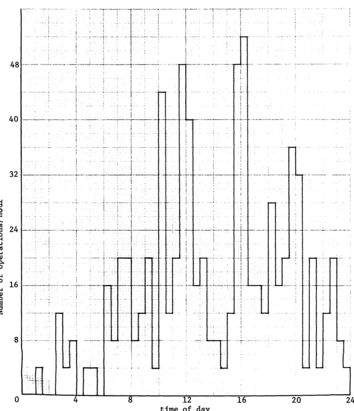
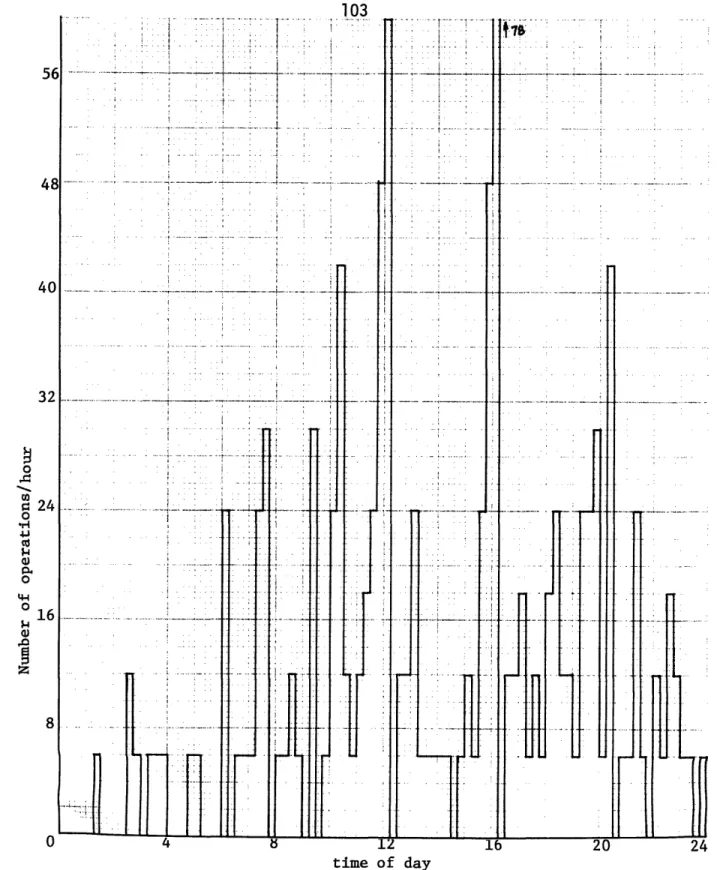
The 24 Hour Demand Profile of Atlanta's Airport Twice the 24 Hour Demand Profile of Amsterdam's Schiphol Airport (recorded at hourly intervals) Comparison of Equilibrium Analysis and Exact Solutions of the Time Dependent Delay for the Demand of Figure 4.2

Twice the 24 Hour Demand Profile of Amsterdam's Schipol Airport (recorded at half hour intervals) Twice the 24 Hour Demand Profile at Amsterdam's Schipol Airport (recorded at quarter hour intervals)

Page No. 6 11 45 86 150 11 16 16 25 40 40 41 91 92 96 102 103

Figures 4.6 4.7,8 4.9,10 4.11,12,13,14 4.15,16,17,18 4.19 4.20

Comparison of the M/M/1 and M/D/I System Delays for a Three Interval Time Dependent Profile Response of E[W(t)] for M/M/1, M/E /1, M/D/I to

the Conditions p = 0.8 j = 1/minuti E[W(O)] = 0

Response of E[W(t)] for M/M/1, M/E /1, M/D/1 to

the Conditions p = 0.7, 0.9, p = 1minute

E[W(0)] = 0

Comparison of M/M/1 and M/D/1 E[W(t)] to Diffusion Approximation under the Conditions p = 0.7, 0.8,

0.9, 0.95, p = 1/minute, E[W(O)] = 0

Comparison of the Relaxation of E[W(t)] to Equilibrium from Various Initial Conditions

for p = 0.7, 0.8, 0.9, 1.2, p = 1/minute

Response of E[W(t)] for M/M/k, k = 1, 2, 3 to

the Conditions p = 0.8, i = I/minute, E[W(O)] = 0

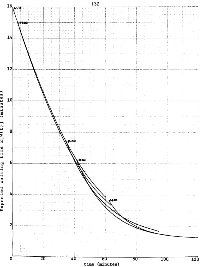
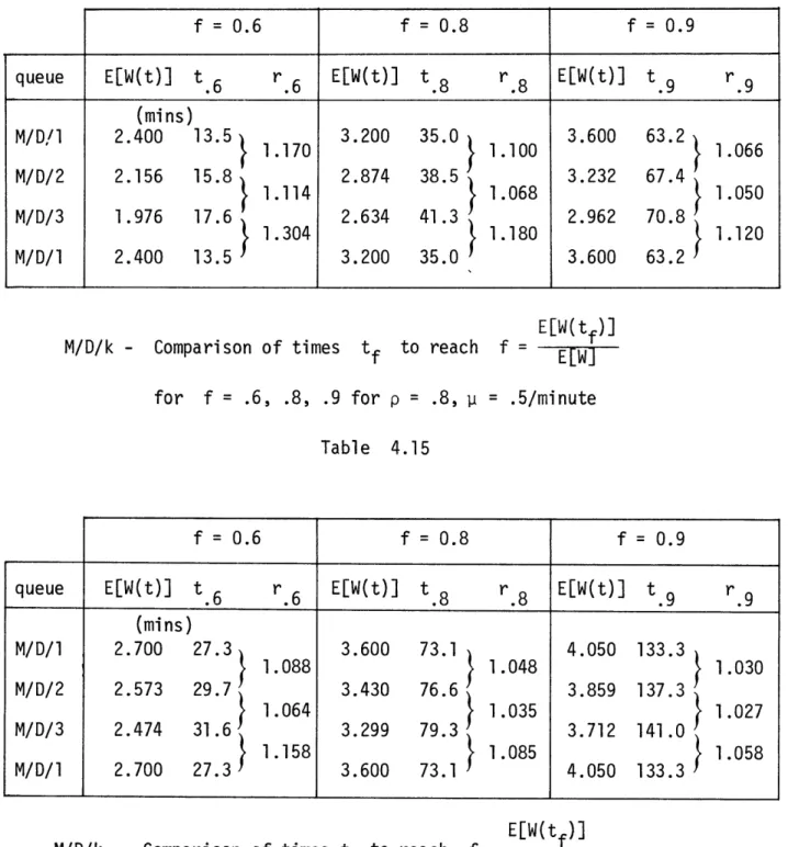
Response of E[W(t)] for M/D/k, k = 1, 2, 3 to the

Conditions p = 0.8, p = 1/minute, E[W(O)] = 0

Page No. 109 116 120 124 132 142 143

Chapter 1 INTRODUCTION

This thesis investigates a service facility with a strongly time varying Poisson arrival rate and service times governed by some general pdf. This is referred to in Queueing Theory as the M/G/k queueing system. The simultaneously probabilistic and time-dependent nature of the arrival process, as well as the "general" character of the service process render this problem impossible to solve by analytical means. The aim here, therefore, is to obtain good approximations and descriptors of system behaviour rather than exact closed form solutions.

The time-dependent M/G/k queue is studied here in the context of airport runway usage. It is clear that this is a situation where there are very large social and economic costs associated with providing either excess or less than adequate capacity. Either large tracts of land occupied by underutilized runways or long queues of aircraft in the air waiting

landing clearance are costly, as well as socially unacceptable conditions. We are concerned here with the busiest of airports - handling large number of scheduled aircraft every day of the year. The time dependency of the demand in these airports extends beyond the presence of morning and evening (or similar)travel peaks common to all transportation systems. Weekly and seasonal demand variations are also very noticeable and extremely impor-tant. Further time-dependence is also introduced by the airport authorities themselves who may schedule additional capacity during traffic peaks, by utilizing more runways than during off-peak periods. Weather,

as well, in the case of airports, has a highly varying effect on capacity. Consequently it is evident that no single queueing analysis of any airport

system can be expected to model this situation accurately except for a fraction of the time. The need for efficient computational methods is therefore apparent.

There are two common criteria for judging the level of service

provided at a facility, both of which are extensively used by aviation authorities. These are the average waiting time per aircraft (clearly as a function of the time of day) and the fraction of aircraft delayed for an amount of time greater than some time to, (also as a function

of time of day). The first of these is the readily available from existing queueing models and in addition forms a base for many other frequently used statistics - total daily delay, annual delay and annual delay cost. Chapter 2 therefore discusses the numerous approaches that have been suggested for determining the expected waiting time in a time-dependent M/G/k queue. In approximately their historical order of appearance, 5

models are presented. The first is the traditional approach of simulation. The remaining four models are obtained by relaxing various conditions of the time dependent M/G/k queueing system. Of these, the first two (Newell [11]) _{are firstordermodels in the sense that they either ignore the} proba-listic nature of both the arrival and service processes or their time-dependence. Second order models, (Gaver [1], Koopman [ 8]) to these are constructed by including both of these conditions but making other assump-tions on their probabilistic characteristics. With increased accuracy, however, comes a substantial increase in computational effort required.

As these latter two models are developed the concept of the transient behaviour of the expected waiting time becomes important as a unifying concept between them. This is because the strong time dependence of the utilization ratio p (ratio of demand to service capacity) rarely allows the system to remain in equilibrium. Chapter 3 therefore addresses the problem of seeking the descriptors of system behaviour (in our case the expected waiting time) when the system is not in equilibrium.

We start by presenting exact models (Morse [ 9], [10]) for the tran-sient behaviour of both the finite and infinite queue capacity M/M/l sys-tems. When the forms of the two results are compared we conclude that, as expected, large finite capacity queues behave in the transient state not much differently from infinite capacity queues. The major outcome of this analysis is a single time constant for the M/M/l system that is valid for all values of p > 0.

At this point in the analysis, we recall the approximating model of the M/G/1 queue given by Gaver and presented in Chapter 2. The time con-stant of the M/M/l system as determined from this model is shown in fact to coincide with the time constant from the exact model. This allows at least some theoretical justification for accepting the time constants from the approximating M/G/l model as the true values for the M/G/l queue.

Based on this we then relate the general properties of the relaxation time of the expected waiting time of an M/G/l queue to its equilibrium value.

Chapter 3 concludes with the presentation of two other models. The first is an approximating model (Gupta [4]) of the time-dependent M/G/k queue that expressly needs analytic forms of the time constant just described. The other model (Clarke [15]) is just an alternate form of the exact transient behaviour model of M/M/1/o given by Morse [9]. After we indicate how to modify this model to remain valid for p > 1 this form becomes just as useful and computationally much more efficient

than the model for M/M/l/m presented at the beginning of the chapter. In Chapter 4 we first give a case study to which we apply three of the models discussed: equilibrium analysis (a first order method),

Koopman's model and the last model given in Chapter 3. We discuss the relative merits of the models and the specific applications to which each

is likely to be most useful. The transient behaviour of queues is ultimate-ly shown to be responsible for the considerable success of Koopman's method.

Then in the next two sections, we pass to numerical analysis of the transient behaviour of the expected waiting time for single and multiserver queues under specific conditions. For the single server queue we first compare the observed time constant to its exact value. Then the observed relations between the transient behaviour of the expected waiting times of various M/G/l queues are compared to the behaviour predicted by the approximating M/G/l model. For the multiserver queue we first give some analytical results (Morse [9]) from which we obtain an approximate

evaluation of the time constant for these systems. Again numerical comparisons are provided to verify these. A brief comparison is also

made between the relaxation times of M/M/k and M/D/k systems as k increases from 1.

As will be indicated all along, the transient behaviour of queues is a controlling factor in the modelling of time dependent M/G/k queues. The analytic and approximating expressions for the time constant as given in Chapter 3 and the numerical experience of Chapter 4 should provide a sound basis for extending the modelling and numerical analysis of time-dependent M/G/k queues.

11 Chapter 2

FIVE MODELS FOR THE TIME DEPENDENT M/G/k QUEUE 2.1 Airport Runway Queuing Systems

We illustrate the generic attributes of queuing systems in the context of airport runway use in Figure 2.1

overflow arrivals

Im

1

.7

.

-.

111

Schematic diagram of airport runway use Figure 2.1

We define the arrival process with aclass of time dependent demand profiles described by the inhomogeneous Poisson pdf with average (time dependent) arrival rate X(t). The Poisson assumption on the arrival

process which has been extensively used in the study of airports accounts for the randomization of actual "arrival" times at the server due to

runway ±

I runway 2 ₁

12

various ATC factors. The time dependence for the larger more congested airports reflects the traffic peaks common to transportation systems and,

generally, is cyclic with a period of 24 hours.

In _{contrast to the arrival process, we will not assume a "neat"} proba-bilistic characterization of the service process. This is motivated by the fact that aircraft service times are neither completely regular (different aircraft have different service times) nor completely random (there do exist standard ATC practices). Also, since the mean rate of service changes infrequently during the course of the day, we assume for simplicity that

the service process operates at constant rate i(t) = p. The service process

defined by these attributes is called the "general" homogeneous service process.

Throughout the mathematical analysis, whenever the number of servers k (runways) is greater than one, they will be assumed independent and identical. They will operate with a single queue governed by a "first-in, first-out" service discipline. Except in very special cases,l this is not a serious misrepresentation of airports.

In summary, we have outlined a time dependent M/G/k/m (k < m < o)

queuing system in the context of airport operations. All of our subsequent examples will draw from airport situations. The arrival process which is simultaneously probabilistic and time dependent, as well as the "general" character of the service process render this problem impossible to solve by analytical means. The aim, therefore, is to obtain good approximations and

1 _{Such as the case where a certain class of users (e.g., general aviation)} commands exclusive use of a particular runway.

descriptors of system behavior rather than exact closed form solutions. To this purpose, we shall discuss or describe in this and the following chapters a number of mathematical models and approaches. Five of the total eight models will be discussed here in Chapter 2. We will refer to them by number from the list as follows:

Model 1: Computer Simulation, M/G/k

Model 2: Time Dependent "Fluid" Approximation, D/D/k Model 3: Equilibrium Analysis M/D/k, M/M/k, M/E /1

Model 4: Stationary Diffusion Approximation, M/G/I

Model 5: Time Dependent Chapman Kolmogorov Equations, M/M/k, M/D/k The first model is the traditional and only non-analytic approach to the time dependent queuing problem. The second is a deterministic model -it ignores the probabilistic nature of both the arrival and service processes, relying entirely on the time dependency for the estimate of the delay. We contrast this immediately to Model 3, equilibrium analysis, which uses fully the probabilistic characterizations of the queuing system processes but ignores the time dependency. The estimates from Models 2 and 3 will be valuable for both the lower and upper bounds they give for delay as well as for providing the groundwork for more sophisticated models. Models 4 and 5 are the extensions of 2 and 3, respectively. The key to these extensions turns out to be the transient behavior of queues which is the central concern for the models to be discussed in later chapters. (Models 6, 7 and 8 are heavily dependent on transient concepts and hence will be omitted from this chapter.)

2.2 Model 1: Computer Simulation, M/G/k

A most accurate representation of a runway queueing system can be obtained through use of a simulation model. The simulation user though pays heavily in terms of computational effort for the additional detail. Each simulation run includes essentially the same computations as those for a single Model 2 estimate, with the addition only of sampling from probability distributions for interarrival and service times. (The assump-tion of course is that these probability distributions are available and empirically or otherwise verifiable.) For practical purposes, however, because of the sampling, one simulation run provides no more statistical evidence than a single day spent in observing the actual airport. The number of simulation runs needed to provide statistically reliable data must then be large and depends on the stochastic properties of the inter-arrival and service time probability distributions. In cases where many airport configurations and demand patterns have to be considered this

approach is then quite impractical. Moreover, Koopman [8] showed that the number of computations in Monte Carlo simulation increases as the square of the desired statistical precision. This is to be contrasted with an

increase which is proportional to the logarithm of the relative precision for the direct solution approach (Model 5).

2.3 Model 2: Deterministic "Fluid" Approximation, D/D/k

We have mentioned that the airport queueing problem exhibits a strongly time dependent arrival rate X(t). Frequently, although not always,

this X(t) contains "rush-hours" where X(t) increases to a point exceed-ing the service rate of the facility and then subsides. In these situ-ations, the analysis of delays has frequently been conducted with the aid of deterministic queuing models of the type D/D/k. Such a model essential-ly needs two variables, the actual cumulative number of customers entering the queuing system, A(t), and the actual cumulative number of customers leaving the system, D(t). If the interarrival and service times were deterministic then the model would be exact. Since, however, in most real systems the arrival and service processes are stochastic, the "deter-ministic" approximation is obtained by assuming that the actual number of operations is exactly equal to the expected number of operations, i.e. that

A(t) = E[A(t)] D(t) = E[D(t)]

D/D/k analysis is customarily done graphically (Figure 2.2). The curve E[D(t)] is superimposed on the curve A(t) . Cumulative delay is then easily calculated by the time integral of the vertical difference of the two curves over the period of interest.

:es

time (minutes)

An example of graphical analysis to solve _{D/D/k systems} Figure 2.2

This method is particularly attractive, computationally, if the number of customers is large. Then on a coarse scale of measurement the queueing queue when A (t)/\-(t) and ý(t) decreasing

tes.

S=L ( t-) dA(t)

dt

=t o

lO00

Example of "fluid approximation" in graphical analysis of D/D/k systems Figure 2.3 10

M

-I

model treats customers as a continuous fluid that is flowing into a res-ervoir at some rate dt A(t) (Figure 2.3). The maximum flow rate out is. the service rate p:

dE[D(t)] 1 dt

As long as dA(t) remains less than the maximum service rate, i.e. dt

X(t) < p, we approximate the queue to be zero. A queue exists between time

t0 when X(t) first exceeds p, and time t1 when A(t) first again equals

E[D(t)].

The consequences of ignoring the statistical fluctuations inherent in the random functions of time, A(t) and D(t), are of course non-negligible. The deterministic model assumes that the server works at a rate p from the beginning of the rush hour until A(t) and E[D(t)] are again equal. In a real queuing process, even under heavy traffic conditions,

there is a significant finite probability that the server remains idle. Service in reality proceeds at a rate p whenever a queue exists, and is

interrupted otherwise. Thus, the real average service rate over the

1. The method does not actually require a constant maximum flow rate p.

The maximum flow rate, just like the average arrival rate,can be time dependent, i.e. p = M(t). Nothing would change in the following discussion under the assumption of a time dependent maximum flow rate.

rush hour can never exceed P, and as we have pointed out, is expected to be somewhat less. On account of this loss of system capacity we expect a nonvanishing queue even when X(t) < p for all t. The D/D/k model, however, ignores the presence of a queue for p(t)= X(t)/vp< 1, and this underestimation of cumulative delay is nondecreasing in time for the duration of the period of interest.

The simplicity of the D/D/k approach, however, has led to its

adoption by the FAA in a real time system for anticipating and preventing 1

large delays to scheduled traffic due to inclement weather. As in these situations the system will almost always be in the oversaturated, p(t) > 1,

state, the queue is likely to grow rapidly in time, making it less likely that statistical fluctuations could allow the queue to vanish. This would

tend to support empirical evidence that themodel performs adequately in these situations. However, in other than rush hour situations, by ignoring the stochastic nature of the arrival process, we disregard, in effect, all of the known queuing phenomena which actually take place on an everyday basis at major airports.

1. Developed at the Transportation Systems Center of the DOT for the Flow Control Facility of the FAA in Washington D.C.

2.4 Model 3: Equilibrium Analysis, M/D/k/c, M/M/k/o

The governing integro-differential equations for M/G/k/o queuing systems are very complex. Therefore, even the simplest case when

the system is in equilibrium does not yield queuing theoretic statistics in closed form. A single exception to this involves the expected steady state delay E[W] for an M/G/1/c system, which is given exactly by the Pollaczek-Khintchine formula:

E[W]

=

-

1 + 2

1

₁

P <

1

(2.1)

91

where s is the random variable described by the service time distribution, and gi is the ith moment of the random variable s.

For some _{special cases of the M/G/k/o queue, with well-behaved} service processes,the governing equations do turn out to be relatively easy write and solve analytically. For these cases the state probabilities and other statistics obtainable from the state probabilities (expected waiting times, etc.) can be derived from the governing equations. In particular, two cases that have received much attention in this type of analysis are the M/D/k/o and M/M/k/c queuing models. These are in fact extreme cases since service times are constant for the first while "perfectly random" for the latter. (The negative exponential pdf, governing the service process in the M/M/k systems, is frequently called "perfectly random" because of its property that at no matter what point in time we observe the process, the time until the next completion of a service is completely independent of the past history of the system). Furthermore, it turns out from the evaluation of (2.1) that E[W] for the M/D/1/cp system is exactly one

half of that of the M/M/l/M system, independent of p or pi. If we accept

the intuitive proposition that individual aircraft service times must be "less regular" than the perfect regularity of constant service time, yet "less random" than the "perfect randomness" of the negative exponential

service time, then we have shown that the delays for M/D/l/o and M/M/l/o

systems provide lower and upper bounds on the true value of delay in an M/G/l/o system. Although no similar relation to (2.1) is available for

the multiserver queues M/D/k/o and M/M/k/o, the closed form formulas for

E[W] of these systems are available and again provide bounds on the M/G/k/o delay.

2.4.1 Poisson Arrivals, Deterministic Service (M/D/k/o)

When service time is of a deterministic nature, for the purpose of making the analysis tractable, the servers are assumed to be identical and to always commence and terminate service simultaneously at equally spaced discrete points in time. These separating time intervals are

exactly equal to the service time of -, where p is the service rate

(operations/unit time) of a single one of the identical k servers. At the designated points in time the model will discharge k or fewer aircraft from service, depending on the number of aircraft in the system, and observe n new aircraft arriving into the queue with probability a(n) given by the Poisson probability distribution

a (,_{t)n e}-_t

a(n)= ,n n = 0,1,...

We then define the state probability Pi(t) as

The recursion equations relating the state probabilities, known in the literature as the Chapman-Kolmogorov (C-K) equations, for any and all dis-crete instants of time are given by:

1 -•s Po(t + = e e) qsk(t) XJ Xj- -1 (2.2) j es j-1 s pj(t + 1 = qk(t) + s e -s pj + (js j! k P(j- Pk+jk+)! (t) + .t) + e pk+j

1

<j

where the following notational conventions have been adopted:

S= (t) * [one service interval] = X(t)

k

qk(t) = Pi(t)

i=O

It is possible for stationary X to solve the system of equations (2.2) for the steady state probabilities Pi(t) and other queueing statistics. Of particular interest here is the steady state expected waiting time E[W]. Saaty [12] gives for the arbitrary server M/D/k/c queue:

E[W] =

,

e-ipk

(ipk)

1_

(ipk)E

i=l

j=ik

!

P j=ik+l

J

p = - < 1

2.4.2 Poisson Arrivals, Negative Exponentially Distributed Service, (M/M/k/o)

Alternatively consider the case of a probabilistic service process with a negative exponential pdf for service time duration (maintaining Poisson

the M/M/k/o system are as follows:

p₀(t + At) = (1 - XAt - iAt) p0(t) + Atpl (t)

pj(t + At) = XAtpj_l(t) + (1 - XAt - jpAt) p (t) + (j+l) vjAtpj+l(t)

1 < j < k-I

Pi(t + At) = XAtPj_l(t) + (1 - XAt - kjAt)pj(t) + kpAtpj+l(t)

k

<j

Passing to the limit, as At O, we obtain from the difference equations Kolmogorov's forward differential equations:

dpo(t)_{dp(t) Xpo(t) + pPl(t)} dt dp.(t)_{dt -t Xpjl(t) - (1+} J-) _{pj(t) + (j + 1) •Pj+l (t)} dt 1 < j < k-I dp (t) dt pj-_l(t) - _{(X + ki) pj(t) + kljpj+l(t) k<j (2.3)} As for the M/D/k queue, closed form expressions for the pi and E[W] are available. For the arbitrary server M/M/k/o queue:

p(kp)k

E[W] = 2 Po

Xk!(l-p)

P -

_k'P

p k1

_L

_n=

₀

n

_{+n l-}

I

kp)k

2.4.3 Application of Equilibrium Analysis

The main problem with the application of equilibrium analysis to the airport queuing problem is that although it correctly recognizes the problem as stochastic, it really is valid only when X(t) is invariant, or varies extremely slowly with time. Even then, the equilibrium approximation with a constant X must be made over a sufficiently long period of time so as to dominate any transient effects. Examination of the demand profiles of the airports most likely to exhibit uniform traffic throughout the day (which are generally the most congested airports, such as New York's LaGuardia, where a quota system on operations is in effect) indicates significant peaks and valleys that seem to invalidate the steady state approach except as a very rough first order approximation.

Furthermore, situations where demand equals or exceeds capacity require special treatment. Up until now, we have been using infinite queue systems.

Equilibrium analysis is invalid for these systems when p > 1 because the queue length is not approaching any limiting steady state value. We could partially circumvent this by considering finite queue systems of large maximum length m.1 This ensures a finite value of delay for all values of p and furthermore, it is a good approximation of the infinite queue system when p < 1. We illustrate this property for the M/M/l/m and M/M/l/o cases.

1 It is by choosing m to be large that we are, later in this study, able to model systems with infinite queue capacity on the computer (i.e., to

The closed form equilibrium state probabilities for these systems,

P

_{and P.}

11

respectively, are known and simple to compare:

finite queue:

pT = (1-p

p

1 l-p

infinite queue: Pi = (1-p)pi P < 1

Clearly, for p < 1, the lim (₁-pm+l) = 1 and

lim P = P. (2.4)

1 1

On the other hand, when p

>

1 in

a finite queue capacity system, the

delay analysis hinges on the fact that there is

a large probability that the

queue is

saturated. When this happens, aircraft "arriving" into the queue

are being forced to cancel operations altogether. As a result, the waiting

time obtained from finite queue analysis will be less than the true value of

delay in

a system where actually all aircraft are served. We conclude that

waiting time in

the queue may then no longer be a sufficient descriptor of

system performance.

Unfortunately, the approximation of an infinite queue capacity system

by finite queue capacity system cannot be extended to the M/D/k case, simply

because there are no closed form results. Therefore, inevitably, in

cases

where temporary oversaturation does occur, the estimating of delays with

equilibrium analysis reduces to educated guesswork on the period of time and

level of oversaturation. It

appears that for the very intervals of time

when the most significant delays occur at our major airports, the steady

state models provide only a very crude approximation.

2.5 Model 4: Stationary Diffusion Approximation M/G/l 2.5.1 Motivation and Assumptions

The deterministic or "fluid" approximation treated in Model 2 should be considered a "first-order" approximation. A "second-order" model is the diffusion approximation model which is the main topic of this section. Whereas the deterministic approximation relied only upon the expected values of the parameters X(t) and p(t), the dif-fusion approximation requires also the second moment of the service process. We review here the analysis by Harris [61 to obtain E[Wd(t)] > 0, the

expected waiting time in queue for a customer arriving a time t after a step demand has been turned on at t = _{0. The service facility consists of} a single server characterized by a "general" stationary service process, with first and second moments of service time gl and g.2

E[W

(t

(a) Step demand at a service facility applied at t = 0 (b) Response of system to given input.

Figure 2.4

Model 4 will differ substantially from the previous three models in the sense that we will define a new state variable. Previously, we used q(t), the queue length, or the probabilities Pi(t) of queue length i, as the state variables. For systems with the particular service processes we have discussed so far, these were state variables because knowledge of their values alone was sufficient to determine probabilistically all future states of the system. For example: (a) With the deterministic service process we discretize time into intervals of single service time length. Then the departure time of a customer from service, given that the customer is in service now, is always the beginning of the next interval, which is entirely independent of the system history. (b) With service time governed by the "perfectly random," negative exponential pdf, we have the Markov memoryless property. Therefore, by definition, the time to next departure from service is completely independent of system history at all times.

In the case of the "general" service process, the probability of a departure from the system in any instant is no longer independent of the system history. We seek then to construct a simple new state variable, one which hopefully would possess the Markov property. Our experience with the differential equations of Models 3 for systems possessing the Markov property indicated that treatment of such systems was considerably simplified by this property.

arriving at time t. This is the virtual waiting time proposed by Takacs as a state statistic. The basic shape in time of a W(t) path of a queuing system (with infinite waiting room) is a random sawtooth. W(t) increases with vertical jumps of independent identically distributed

(iid) service time magnitudes at the instants of customer arrival while continuously decreasing deterministically at slope -1 whenever the queue is nonzero.

The W(t) path so described is both additive and Markovian. Since

the arrivals follow the Poisson process, the next arrival will, independent-ly of the past history, occur on the basis of an interarrival time with negative exponential distribution with (possibly nonstationary) mean . All arrivals, independent of the state of the system, cause jumps in W(t) of height given by iid random variables which are distributed as the ser-vice times of the system.

In addition to the additive and Markovian properties of W(t) we make two key assumptions on W(t) prior to presenting the diffusion model. The first assumption requires that changes in W(t) in a small time interval be negligible with respect to W(t). Due to the jumps observed in W(t) this requires that the queue always contain many customers as well as W(t) >> gl. In general, W(t) remains large, and the first assumption is satisfied when p is "close" to unity. As the model parameters are defined, the implications of, and measures for "closeness" will be made more precise.

The second assumption hypothesizes the existence of an infinitesimal time interval T, short enough to allow W(t) to change only by a negligible

amount, but simultaneously long enough for many events to take place in T. (The mean interarrival time must therefore be short when compared to the time scale of the approximation.) This allows us to invoke the

Central Limit approximation of sums of random variables. Were it not for the condition W(t) > 0, then W(t) could easily be obtained by adding sums of independent normal random variables (of waiting time) correspond-ing to arrivals and departures from the queue. Also it is clear that invoking the Central Limit Theorem causes the discrete component of W(t), the number of teeth in the random sawtooth, corresponding to the Poisson arrivals, to be modelled only approximately.

2.5.2 Model Development

In the following discussion we will describe the (conditional)

transition pdf f(x,t

IxOt0)

for the waiting time x in

the system

at time t, given that it was x0 at t0 a short time earlier. As

postu-lated, x is described by a continuous transition Markov or diffusion process. This approximation method to the waiting time problem is governed by the

partial differential equation of the Weiner process:

af af b a 32f

at = -a(t)-x _ax + ₂ (2.5)

This process has the property that it is completely specified by the parameters a(t) and b(t) once :initial boundary conditions are set. a(t) and b(t) correspond to the infinitesimal mean and variance of the motion of the process. They are given by:

a(t) = T-1E[W(t + T) - W(t)]

b(t) = T-1 Var[W(t + T) - W(t)]

Now a(t), b(t) can be readily computed because of the Markovian property

of W(t). Only two events are possible in time T - no arrival (and the

waiting time decreases by T), or an arrival (and the waiting time increases by random variable s, from the distribution of the service times, less service completed on the customer in service, T)

E

- a(t) glx(t) - 1

Var[W(t + T) - W(t)] (t)-rg ₂ = Tb(t)

=> b(t) _{= X(t)g}

2

The boundary condition is simply f(O,t) = 0 t > 0

Although there are many possible solution methods to this problem, the most commonly cited approach is the method of images from physics (Harris [6], Gaver [5], Newell [11]). For the

stationaryI parameter case ,(t) = X: E[Wd(t)] = 3 2 Xg₂ (g₂X) - (l-g1 ) 2(1-g1X) 2(lg 1 )2t½ e 2g2X 3 gl-l)t + g2 (g) 2( X)2 - e 2g 2 2(glX) 2 2(l-glX)2t½

2.5.3 Characteristics of E[Wd(t)] (Model 4)

It is clear that the expressions (2.6) - (2.8) for E[Wd(t)] from Model 4 differ substantially from the values obtained by the methods of Model 2. The most obvious improvement over Model 2 is that the diffusion approximation predicts a delay for all p > 0, not just p > 1. Another aspect is that E[Wd(t)] agrees at least in form with the behaviour we would expect by solving directly the integro-differential for the M/G/1

1. Harris shows that straight forward application of this method will not

work for nonstationary parameters.

glx< 1 gl = 1 (2.6) (2.7)

(2.8)

system: namely E[Wd(t)] is a composition additively of terms which are functions of time and a term which is a constant independent of time -the transient and steady state terms - respectively.

Before examining the transient and steady state terms we pause briefly to observe why Model 4 is in fact a "second-order" approximation with respect to Model 2. The argument centers on assumption two (and the

Central Limit Theorem) which implies that events during a small interval of time T are normally distributed. Equating the two incremental parameters a(t) and b(t) of the real and approximating (f(x,t)) processes ignores

all higher moments of the real transition pdf. Contrast this with Model 2 which neglects the possibility of fluctuations in events completely, through a law of large numbers argument. This corresponds to the total neglecting of the term b(t) ₂ 2 _x2 in (2.5).

Model 2 had no transient or even steady state component. The only term appearing in the waiting time for both Models 2 and 4 is the linear growth with time: (glX - l)t for p > I. The much more intuitive behaviour of Model 4 will be illustrated in the following. The E[Wd(t)] (2.6) - (2.8) are valid for the case of a step demand X beginning at time t=O, with

initially no customers in the queue. We expect and observe the time dependent waiting time E[Wd(t)] approaching its limiting steady state behaviour from below.

The case p< 1 is the only case that approaches an equilibrium solution with the decay of the transient. For the overloaded queue,

p > 1, not all the customers can be served, causing the queue to grow with time. There is still, however, a transient term. As for p < 1,

the transient decays exponentially, and E[Wd(t)] approaches growth as (gl, - 1)t. The relation for the special case of demand exactly equal-ing the mean rate of throughput also agrees with intuition. Neither an equilibrium solution as for p< l,nor linear growth with time, as for p > 1 ,is expected for E[Wd(t)] when p = 1. The observed growth as A/, slower than for p > 1, indicates the basically unstable nature

of the queue, as expected.

The behaviour of the transient term should be closely examined. Apparently for both p ý 1 the transient term decreases as t½e/to where

to is a constant. Because of the dominance of the exponential com-ponent in t, to has been termed the relaxation time, defined as the length of time required for the transient part of the queui~ng statistic

1

to relax to 1 _{of its original value. Chapter 3 will be devoted entirely}

e

to analytic and empirical treatments of the transient behaviour. There-fore, this behaviour will not be discussed further here. We will, how-ever, quote known steady state results in the next few paragraphs to show that the asymptotic behaviour E[Wd] = lim E[Wd(t)l does reasonably

t-_oo

approximate these results.

The expected steady state delay E[W] for an M/G/l system is given exactly by the Pollacek Khintchine formula (2.1). With the diffusion

E[Wd] = Xg₂ -P _{g2 [g Va [s]] E[W]}

2(1-p)

2(l-p) 1

2(1-p) 1

9

The expected values are therefore exactly equal. The exact expression for the variance of the waiting time is

Var[W] = 'g2 2

2

_(1-p)

Xg₃

6(1-p)

To obtain Var[Wd] we return to the original differential equation for the diffusion process:

af af b(t) 2f

t a(t) +

2 ax2

For the stationary case a(t) = a = constant, b(t) = b constant, we

af

can set =t - 0 and solve for f, the density of the waiting time in queue.

The equation is satisfied by:

f(x) = 2_g(l-P) exp [_2(12)x ]

2X gex p< 1

Recognizing this as an exponential distribution we obtain the variance

Var[Wd] _{= E} 2_[Wd]

=

(l-pL

< Var[W]

Therefore, we obtain a smaller variance for p< 1. Gaver I] was able to prove that these do coincide for the case p = 1.

2.6 Model 5: Numerical Solution of the Time Dependent Chapman Kolmogorov Equations, M/D/k, M/M/k

2.6.1 Method and Assumptions

Koopman [8], rather than relying on steady state results, has sought and obtained numerical solutions for the Chapman-Kolmogorov equations for M/D/k and M/M/k systems. Since the queuing equati:ons are valid for all values of p (not just p< 1), iterative numerical solution of the equations yields the distribution of the queue length Pi(t) i = 0,1,... from which the expected delay E[W(t)] is calculated. Further it is possible to adjust the average arrival or service rates at any iteration of the numerical solution of the equations to reflect any corresponding variations in the "real world." (Frequently airports operate with fewer runways at nights or during bad weather. This situation can be accomodated in the numerical solution.)

Koopman has shown that, in the absence of steady state conditions, periodicity of the X(t) and -p(t) usually observed at airports (diurnal 24 hour schedule pattern) guarantees the existence and uniqueness of

the state probabilities Pi(t). These solutions for the state probabilities will be valid as long as (a) the average service time - of an aircraft is small enough such that no significant change in arrival rates or general conditions is observed during a single service time and (b) there exists during the day a period when the level of operations is negligible compared to the airport capacity. This point must be chosen as the starting point

so that transient considerations remain negligible. In the event that such a point does not exist the Pi(t) should be evaluated over a period of time equal to twice the cycle of the X(t) to ascertain that periodicity is indeed achieved. For practical purposes, however, this issue is not particularly important. The remaining basic assumptions of this approach are identical to those presented in section 2.4. Koopman developed the one runway case assuming a finite maximum queue length (since numerically it is possible to solve only a finite number of state equations). No distinction was made between arriving and departing aircraft, although possible extensions to multiqueue situations were illustrated.

2.6.2 Computational Considerations

Minor changes must be made to the last k equations in (2.2) and (2.3) when there are only a finite number of states m. These are to ensure that the maximum queue length is not violated by the number of new

aircraft arriving into the queue,as well as to ensure that the probabilities add up to 1. For the M/D/k system the last k equations are:

j -Xs j-1 - j-(m-k) -Xs 1 X e s e e pj(t + ) = qk(t) + s s p (t)mk+l j! (j-1)! [j-(m-k)]! m - k< j< m-l 1 =qk(t _{+) + Pk+l (t +) + + m(t + 1} k~t + 1 1

36

dp (t)

= MPj-l(t) - (X+ kP)p (t) + kp pj+₁(t) m - k< j m-l dt

1 = p0(t) + Pl(t) +...+ Pm(t)

According to the discussion of Model 3 we would like m to be large enough such that queue saturation never takes place. Bearing in mind

the strongly time dependent X(t) (and/or lp(t)), we realize that in the

course of an iterative solution the value of m for which pm(t) becomes negligibly small can vary appreciably. Much computational effort may be saved by recognizing that negligibly small probabilities need not be

calculated. Thus a fictitious "maximum allowable" queue length can be set up to vary at each iteration in a fashion to ensure that the proba-bility of queue saturation does not exceed a negligibly small predetermined tolerance.

Given then a set of initial values pi(O) i = O,l,...,m, and the

average arrival and service rate profiles X(t) and p(t) for a time period

of interest [0,T], the equations can be solved for the queue length distributions at discrete points in time for the interval. For the M/D/k case the distributions obtained correspond to points in time i-t)

(=1 aircraft service time) apart. The M/M/k equations must be solved

as difference equations and consequently yield the solutions at arbitrarily small, but regular, intervals of time At.

2.6.3 Application

The statistic usually of greatest interest, the expected waiting time in queue ,E[W(t)],is readily obtained once the pi(t) are known:

m

E[W(t)] = kt (i-k+l) Pi(t) (2.10)

A minor change to (2.10) must be made for the M/D/k case to account for the modelling hypothesis that all arrivals into, and all departures from the system occur at discrete instants of time:

1 m 1

E[W(t)M/D/k k-(t) k (i-k+-) p(t)

Other measures of importance, the expected queue length, m

E[L (t)] = E (i-k)pi(t)

i=k

and probability that an aircraft is delayed prior to service, k

P(W > 0) = 1 - Pi (t)

i=O

are easily computable.

Koopman discovered that delays observed in systems with A(t) strongly time dependent were remarkably insensitive to the precise

stochastic properties of the service process.

Also, we have noted in our discussion of steady state results, from the Pollaczek-Khintchine formula for the single server queue, and closed form expressions for many server systems, that M/M/k and M/D/k systems appear to provide upper and lower bounds on the average equilibrium delay. Together these observations imply a tremendous simplification of the

study of the M/G/k queue. Koopman's results suggest that judicious inter-polation of nonequilibrium M/D/k and M/M/k solutions is all that is needed to obtain a good approximation of actual delays in a nonstationary M/G/k queuing system. Similar closeness of the variances of the expected queue lengths (the variances tend to be large compared to the difference of the expected queue lengths for the two different service policies) further strengthens the case for the validity of interpolation.

2.6.4 An Alternative to Interpolation

We conclude this section with a brief investigation of a mathematical-ly tractable alternative to interpolation between M/M/k and M/D/k delay statistics in obtaining the delay for M/G/k systems. At least part of the success of Koopman's solution technique is due to the fact that

these two extremes have the simplest forms of the C-K equations (2.2) and (2.3). We will now investigate the efficacy of numerically solving C-K equations when more general service processes are introduced. In particular we write the C-K equations for a class of service processes that includes both the deterministic and negative exponentially distributed

service times as its extremes. The outcome will be that even for the simplest case of a single server, numerical solution of these equations fails to be practical when compared to Koopman's method.

The class of service processes we mean is the cth order Erlang

distribution whose pdf f(s), for an arbitrary integer c > 0, is given by:

(c)c c-1 -c0s

f(s) s e s > 0 (2.11)

(c-l)!

By definition f(s) is the distribution of the sum of c iid exponential random variables x, f(x) = cpe-c x, . x > 0, each x having mean c. Therefore, the mean service time and variance of s are:

1 1 g = c . - -(2.12) 2 1 1 Var[s] = c = c - = x (c 1) 2 c-2

From (2.11) and (2.12) it is obvious that both negative exponentially distributed and deterministic service times are special cases of service time described by the cth order Erlang pdf, with c given by 1 and o respectively.

For the purpose of writing the C-K equations of a single server queueing system with service process defined by the cth order Erlang pdf

(still with Poisson arrivals) abbreviated as M/Ec/l, we note that although the Erlang distribution itself is not Markovian, the distribution

is composed of c lid negative exponential units. We call these units "phases" and imagine a queueing system with cth order Erlang service time distribution as the "c phase service" queue illustrated in Figure 2.5:

overflow

₁

_{1 1}

1

0-

/Luzz.

.

fie

"arrival" finite queueing service

process space process

A schematic diagram of the cth order Erlang type service queue Figure 2.5

The effect of increasing the number of phases required by each customer, i.e. going from "perfectly random" to deterministic type service, on the

distribu-tion of the service times is shown in Figure 2.6.

A,

4J

Oi

O S2

ju t o0

(1-cumulative distribution function) of the cthorder Erlang pdf(Morse[lO]) Figure 2.6

41

We take advantage of the description of service as "phased _" by measuring the queue length in terms of phases remaining to be com-pleted, rather than the total number of waiting customers. This is easily done as the arrival of every customer corresponds to the bulk arrival of c phases of service. The state diagram for the M/E3/1 queue, in terms of the phases is given in Figure 2.7. As each phase possesses the

xAt At xAt _At xAt

31 31' 3 311 3-1

State diagram for an M/E3/1 system Figure 2.7

Markovian property the state transition probabilities are independent of time. The differential equations fore pi(t) = 0,1...., the probability of i

phases of service remaining to be completed at time t, are then written as in (2.3):

dpo

dp0 -Xp0 + c.- P1 dt

dpi

dt -(c + cp)Pi + cl.Pi+l O< i < c (2.13)

dpi

The numerical solution of the equations (2.12) is obtained the same way as for (2.3) although such a direct solution is computationally disadvantageous. The reason, of course, is that the number of states, and consequently the number of differential equations, is c times that of the "equivalent" (in the sense of customers in the queue) M/M/l system. As these equations must be solved simultaneously the increase in computational effort is greater than linear. Solving, for instance, M/E3/1 systems takes about an order of magnitude more computation time than the M/M/l system. However, mumerically solving the M/Ec /l system will provide the exact results for the transient behaviour of yet other special cases of the M/G/l queue (besides M/M/l and M/D/1). Therefore, many results will be presented for this case in the section on numerical results.

2.7 Summary

In this chapter we have reviewed the five main types of models which have been used in the analysis of nonstationary M/G/k queues.

The main objections to three of the models were:

Model 1, Computer Simulation: requires excessive computation time and poses serious statistical difficulties in interpreting results. Model 2, D/D/k "Fluid Approximation": ignores known and observed

statistical fluctuations in both the demand profile and service

times. Predicts no waiting time unless p > 1, and always underestimates waiting time. When compared to exact solutions Model 2 fares

worst when p is frequently less than, but close to, 1. Performance is better when p > 1 and is best for lengthy periods of oversaturation. Model 3, Equilibrium Analysis: fluctuations in airport demand

profiles are very significant with the resultant conclusion that the system is never truly in the steady state. No solution for common "rush hour" situations, p > 1, for infinite queue systems, and difficulties in interpreting the values of E[W] for finite queues

(because of queue saturation).

The fourth model (stationary diffusion approximation) was introduced as a natural extension of the deterministic approximation Model 2. Al-though analysis of delays for nonstationary demand profiles has been conducted with this method (Harris [6]), it is limited to particular

demand profiles and single servers, and hence was not discussed here. However, the results of Model 4 are invaluable in providing approximate closed form results for the transient behaviour of (stationary) M/G/l queues, since exact results exist only for M/M/I.

The most promising method so far is Koopman's method of interpolating between the results of numerical solutions of the M/M/k and M/D/k

systems because:

(1) apparently in time dependent M/G/k systems E[W(t)] is not strongly dependent on the exact form of the general service

process. Therefore, interpolation between the extreme values of E[W(t)], based on theproperties of the service process, is generally sufficient to approximate the true value of E[W(t)]. Besides,

direct solution of the C-K equations for the particular service process was shown to require excessive computation time for even relatively "well behaved" service process such as the Erlang k. (2) it requires substantially less computational effort than a

simulation, and overcomes the difficulties of both Model 2

(when p< 1) and Model 3 (when p > 1) by calculating exact results for all values of p.

The following chapters will offer an explanation, based on theoretical considerations, for the success of Koopman's method. It will also provide a framework for investigating other models that can be developed for the M/G/k system with this knowledge.

Chapter 3

DERIVATION OF THE TIME CONSTANT OF THE M/G/1 SYSTEM AND APPLICATIONS 3.1 Motivation

Until now we have mentioned the term "transient behaviour" infre-quently and each time in a slightly different connection. The first men-tion of it was in Model 3 where we said that the equilibrium approximation could be safely applied only when X(t) has been (nearly) constant for a sufficiently long period of time so as to overshadow any transient effects. Although constant demand profiles are currently rarities for airports, this might change. Setting of hourly quotas on runway movements, and marginal cost pricing of runway use are two of the policy decisions that may at

least partly bring this about. If the resultant policy creates (near) con-stant daily demand profiles, then the application of Model 3 would seem to

provide adequate rough approximations to the delays. Consideration of transient effects will show that this can in fact be misleading. Steady state delays increase exponentially (2.1), as the utilization ratio approaches 1. However, the length of time required to reach the steady

state also increases exponentially. Therefore, both the relaxation time and the actual transient component of E[W(t)] must be known before steady state results can be of any value.

Our second mention of the transient concerned the response of an M/G/l queue, Model 4, to a step demand applied at time 0 when the queue was

1. For average steady state delays per operation in the tolerable range for airports this period of time approaches a length equal to that of the operating day.

initially empty. Closed form results available from the governing equa-tions of Model 4 can be used in creating approximating models of the more complex time dependent queue. For instance, the expression for the tran-sient behaviour is the controlling factor in a computationally efficient methodology developed by Gupta. Based on knowledge of the steady state behaviour and some (incomplete) knowledge of the duration of nonnegligible transient effects, he was able to construct and solve an approximating differential equation for the queue length of time dependent M/M/K and M/D/K queues.

The third reference to the transient was in Model 5 in connection with initial starting conditions. Besides this, the transient plays another extremely important role in Model 5, and we take this opportunity to men-tion it. The reader will recall that the results of equilibrium analysis indicated that the steady state E[W] for the M/M/K and M/D/K queues dif-fered by approximately a factor of 2 for small k. Koopman, however, ob-served that in the numerical solution of the equations the two systems provided relatively tight bounds on the system delay. It is of interest then to investigate the transient behaviour of the M/M/K and M/D/K systems as a cause of this behaviour.

It is clear from the discussion that any progress we make in analyz-ing transient behaviour will be extremely useful. We will start by pre-senting yet another model, Model 6, comparable to Model 4 in the sense that it deals with a stationary queue, with the differences that it is an exact model and limited to the M/M/l case (as opposed to the approximating

M/G/l analysis). Our aim is to obtain some workable expression for the transient behaviour that can be considered exact. We will note the simi-larity of the queueing statistics obtained from Model 6 and Model 4, and make comparisons. Since Model 4 will turn out to be a very good approxi-mation of the stationary M/M/l queue, we make attempts to stretch our knowledge of the "exact" transient behaviour to the gamut of M/G/l queues via the parameters of Model 4. We conclude with Models 7 and 8. The former is an approximation model of the time dependent M/M/k and M/D/k queues which expressly needs the kinds of closed form results that this chapter.

is concerned with. Model 8 uses the development of Model 6 to formulate a new model for the time dependent M/M/l queue. In particular we suggest Model 8 as an alternative to Model 5 when quick approximations are needed.

3.2 Model 6: Transient Solutions for Stationary Queues, M/M/I 3.2.1 Morse's Methodology

This section develops series-form expressions for the transient state probabilities pi(t) for stationary finite queues. The methodology is due to Morse [lO],and is perfectly general provided the arrival and service processes constitute a birth and death Markovian model.

Drawing upon the birth and death process property of the model we are able to write the linear Chapman-Kolmogorov equations. When the sys-tem is not in equilibrium we have the forward Kolmogorov differential equation for the time rate of change of the state probabilities:

dpi(t) m

dt n 0 EinPn(t) (3.1)

where the Ein are the rates of transition into state i given the system was in state n an arbitrarily short time earlier. The E.in are the mean arrival rates of the exponential units, which may in their most general form be themselves functions of time. For the transient analysis, however, all parameters will be assumed stationary.

The analysis begins with the assumption that the transient state proba-bilities we seek, Pi(t), are completely described by the form (3.2):

m -Yst

Pi(t) = E Bise _(3.2)

s=O

49

(b) Bis i,s = 0,1,2,...,m are constants to be adjusted to meet initial conditions

(c) Ys s = 0,1,2,...,m are rates of decay of transient com-ponents

Substituting (3.2) into the differential equations (3.1)we obtain:

Y YiB e it _{+ E}

n=O

EinPn = 0 i = 0,l,...,m

(Yi + Eii)Pi + _Sn=OZ

nOi

EinPn = 0 i = 0,1,...,m

Equations (.3.3)must have solutions for the pi, for all i, yielding

the following secular equation (3.4) in the yi:

(YO + E₀₀) S Elm (y _{+ E} 11) (Yn + Enm) (3.4) = 0

From linear algebra the system(3.3) has a nontrivial solution if and only if the determinant of coefficients (of the pi) (3.4) equals zero. We show

this to be the case for the general birth and death queueing system

from the properties of a Markov process. The rate of transition into

a state always equals the rate of transition out. By definition (from

equation (3.3) above),

-(Eii

+

yi) equals the rate of transition into

state i. Now the column sum of the determinant over all rows j,

j

i

is:

m

SE..

=

rate of transition out of state i

j=0 31

jti

Consequently, the column sum of (3.4) is

0

for every column. It

follows then that the determinant (3.4) is

zero.

The secular equation is

of the (m

+

)st order in

the variable

y.

Solution for the m +

1

roots

ys

yields:

(1)

the zero root, Yo

=

0: the determinant of the coefficients is

zero

and consequently the coefficient of the zeroth power of y,

i.e. the

constant, in

the secular equation is

zero. Therefore, one root of the

equation in

these systems will always be 0.

(2) n positive roots ys,

s = l,...m

When the coefficients B. are adjusted to fit the initial conditions

the pi(t) are readily computable for (3.2) The presence of the zeroth root

implies that the first term in

the expression (3.2) must be a constant

in-dependent of time, i.e. the steady state probability Pi. The remaining

n roots are therefore associated with the transient behaviour of the

system. With a constant term added to an exponential transient term, it should be noted that this behaviour coincides at least in form with the approximating diffusion result given in section 2.5.

3.2.2 Application of Morse's Methodology to the Queue M/M/l/m

For small m the roots yi are readily obtainable from the secular equation (3.4). In the case of large m though, Morse avoids writing (3.4) explicitly. Instead, he obtains the roots by appropriate manipulations of the m + 1 state equations.

The forward Kolmogorov differential equations, written for the single channel case are:

dp0 dtp _{-= Pl(t) -}

_xpO(t)

Assume the transient to be of the form i

2i -Yst