HAL Id: hal-01944514
https://hal.umontpellier.fr/hal-01944514
Submitted on 14 Dec 2018HAL is a multi-disciplinary open access archive for the deposit and dissemination of sci-entific research documents, whether they are pub-lished or not. The documents may come from teaching and research institutions in France or abroad, or from public or private research centers.
L’archive ouverte pluridisciplinaire HAL, est destinée au dépôt et à la diffusion de documents scientifiques de niveau recherche, publiés ou non, émanant des établissements d’enseignement et de recherche français ou étrangers, des laboratoires publics ou privés.
Energy Consumption-Economic Growth nexus in
Sub-Saharan Countries: what can we learn from a
meta-analysis? (1996-2016)
Alexis Vessat
To cite this version:
Alexis Vessat. Energy Consumption-Economic Growth nexus in Sub-Saharan Countries: what can we learn from a meta-analysis? (1996-2016). The 9th Winter Student Workshop of the French Association of Energy Economist (FAEE), Nov 2016, Paris, France. �hal-01944514�
1
Energy Consumption-Economic
Growth nexus in Sub-Saharan
Countries: what can we learn from a
meta-analysis? (1996-2016)
Abstract
The relationship between energy consumption and economic growth remains one of the most debated topics in the economics literature. Studies in this field have been carried out in developed countries since the end of the 70s, but they not have led to consensus about the relationship other than finding four causality directions: unidirectional in two directions, bidirectional, or neutral. This lack of consensus remains one of the most relevant findings on energy issues. During the 2010s, the scope of the studies on this relationship broadened since, for example, energy demand in Sub-Saharan Africa has outpaced that in the North and the IEA has forecasted the greatest increase in energy consumption to come from this area. The relationship between energy consumption and economic growth began to be studied in Sub-Saharan Africa in the late 90s, using the same method as for developed countries and with the same lack of consensus on the direction of causality. This paper attempts to clarify this situation through a meta-analysis of fifty articles published since 1996 to 2016. This meta-analysis involves five analytical categories: type of publication, geographical area studied, econometrics method used, energy consumption indicators, and control variables. Each of these dimensions includes many disaggregated variables. Logistic regressions are run on the variables presented above for each of the four causality hypotheses. In research that studies single countries, the likelihood of finding for a given causality
2 hypothesis is very sensitive to the econometric method implemented. Findings on a panel of countries are then presented; their methods assert the neutrality hypothesis.
JEL Q40, Q49. Keywords: Energy Economics, Economic Growth and Development, Energy Consumption.
I. Introduction
Energy has emerged as one of the key “drivers” of economic development (Sebri, 2015). In the industrialized countries, the magnitude of energy’s influence on economic growth remains a controversial issue (Kraft & Kraft, 1978; Payne, 2010). Nevertheless, macroeconomists agree on the predominant role energy plays. Energy serves not only to improve the productivity of the main factors
3 of production such as capital and labor (technical progress), but also allows a given country to assess whether its own level of development can be considered advanced (Jumbe, 2004). The 2004 International Energy Agency report sheds light on the contribution of energy consumption to economic growth (IEA, 2004). As an explanatory variable, energy consumption is positively related to the level of output in both developed and developing countries (IEA, 2004).
Academics and professional circles have assumed energy to have a predominant role in economic growth (Kraft & Kraft, 1978). However, this relationship has been controversial since the beginning (Akarca & Long, 1979). Interest in this relationship could be understood as a result of the oil supply shocks of 1973 and 1979, raising concerns about the increase in real energy prices or the scarcity of natural resources. However, the most important finding, repeated through a large number of studies, is the lack of consensus on the direction of causality between energy consumption and economic growth. In studies of the causality between energy consumption and economic growth in developing countries, the findings are also conflicted, as the empirical findings on the direction are largely inconclusive. The economic and energy contexts that serve as a framework for investigating the nexus for the Sub-Saharan countries are very singular. Since the early 2000s, the pace of economic growth in Sub-Sub-Saharan countries has been higher than that of the world economy, although this trend is not uniform across countries. Already in 1980-2010, the pace of economic growth in Sub-Saharan countries exceeded that of developed countries, with the exception of the last few years. Since the 1990s, the Sub-Saharan countries have embarked on the structural adjustment plans/policies jointly promoted by both the World Bank and the International Monetary Fund. Major international organizations highlight that before these changes, there had been a dramatic slowdown in real incomes, economic growth, investment, and savings in Sub-Saharan countries, often associated with the rapid increase of public debt. Although heterogeneous, this phase of growth follows a very difficult economic context: the World Bank’s 1989 report focused on the weakness of economic growth in Sub-Saharan countries, where the annual economic growth rate fell from 7% between 1965-1970 to 2.2% during the period 1980-1987. The impact of this economic slowdown created major concerns for oil-exporting countries.
4 In terms of energy, despite a large endowment of natural energy resources, Sub-Saharan countries remain characterized by poor energy supply and small quantities delivered (Wolde-Rufael, 2005 & 2006). Investments in electricity production capacities are insufficient. For instance, between 1973 and 1998, electricity generation in Sub-Saharan Africa grew at a rate of 5.1%, while it grew at a rate of 6% in Latin America, and 7.8% in Asia (8 % in China) (Turkson & Wohlgemuth, 2001). In Sub-Saharan Africa, energy market supply only covers a small part of the needs of the population, even excluding non-market demand, and the gap between electricity demand and supply is continuing to increase. From 2000 to 2012, electricity demand rose by 45%, whereas electricity supply increased by 19% (World Energy Outlook, 2014). At the same time, demand for electricity in Sub-Saharan Africa is extremely fragmented, coming from a limited group of countries, and an even more limited number of people connected to the centralized “on-grid” network. In Africa, the main centers of electricity demand are South Africa and Nigeria, which account for almost 40% of total electricity consumption in the region (World Energy Outlook, 2014).
In this general context, a vast body of published scientific papers on the nexus has accumulated no consensual results and thus cannot inform energy policies although each hypothesis on the direction of causality provides clear policy direction.
The “growth” hypothesis (H1) sees unidirectional causality running from energy consumption to economic growth. This hypothesis states that energy consumption is a prerequisite for economic growth. In this context, energy consumption is a direct input for achieving economic development and an indirect one that complements the main factors of production (Ebohon, 1996; Templet, 1999; Toman & Jemelkova, 2003). In this scenario, the country’s economy is energy dependent (Ebohon, 1996; Templet, 1999; Toman & Jemelkova, 2003; Ozturk & al, 2010). Thus policies favoring energy consumption are likely to accelerate economic growth.
The “conservation” hypothesis (H2) suggests unidirectional causality running from economic growth to energy consumption: Any increase in wealth necessarily leads to an increase in energy consumption. If this hypothesis holds, policymakers could make
5 significant steps to foster energy efficiency improvement, such as reduction in greenhouse emissions and demand management policies (Payne, 2010), without hampering economic growth. The economy in this scenario is less energy dependent.
The “feedback” hypothesis (H3) indicates a bidirectional causal relationship between energy consumption and economic growth. If the two variables influence each other, any energy policies introducing limits on energy consumption will negatively impact the increase of country’s wealth, and any increase in economic growth will lead to an increase in energy demand (Sebri, 2015).
The “neutrality” hypothesis (H4): sees an absence of any causal relationship between energy consumption and economic growth (Ozturk, 2010). In this scenario, energy policies can be implemented without any effects on economic growth.
Published outcomes on the relationships between economic growth and energy consumption in the Sub-Saharan countries can be categorized into two types:
The first group includes studies based on individual countries using time-series analysis (Table 1). These studies use the cointegration test (Engle & Granger, 1987) as well as a maximum likelihood test based on a system-based reduced rank regression model (Johansen, 1988, 1991, 1995; Johansen & Juselius, 1990).
6 Table 1. Summary of the nexus in individual countries in SSA
Author(s) Countries Reviews Methodology Findings
1. Ebohon (1996) Tanzania (1960-1981), Nigeria (1960-1984)
Energy Policy Sims and Engle-Granger causality tests Tanzania: H3 Nigeria: H3 2.Jumbe (2004) Malawi (1970-1999) Energy Economics Sims and Engle-Granger causality tests Malawi: H3 3.Kouakou (2011) Ivory Coast (1971-2008) Energy Policy Sims and Engle-Granger causality tests within an ECM Ivory Coast: H3 Short-run: H1 Vs Long-run: H2
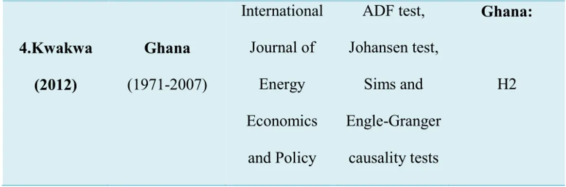
7 A second group of studies uses panel estimation techniques or panel datasets that have been employed to capture country-specific effects (Table 2). We emphasize that Arima (1994) identifies this classification for all developing countries. The panel research takes a different approach, moving from a global to a country-by-country comparison and thus providing more data points compared to a single time series. Panel estimation techniques increase the degrees of freedom and reduce the likelihood of collinearity among regressors (Apergis & Payne, 2009; Levin & al, 2002). Thus, panel estimation techniques overcome the problem of collinearity and endogeneity of explanatory variables. However, the panel research smooths out the differences in structures between countries.
Table 2. Summary of the nexus for a panel of countries in SSA
Author(s) Countries Reviews Methodology Findings H1 4.Kwakwa (2012) Ghana (1971-2007) International Journal of Energy Economics and Policy ADF test, Johansen test, Sims and Engle-Granger causality tests Ghana: H2
8 1. Wolde-Rufael (2005) Algeria, Benin, Cameroon, RDC, Congo, Egypt, Gabon, Ghana, Ivory Coast, Kenya, Morocco, Nigeria, Senegal, South Africa, Sudan, Togo, Tunisia, Zambia, Zimbabwe (1971-2001) Energy Economics ARDL & Toda & Yamamoto causality test Cameroon H2 Algeria, DRC, Egypt, Ghana, Ivory Coast H3 Gabon, Zambia H4 Benin, Congo, Kenya, Senegal, South Africa, Sudan, Togo, Tunisia, Zimbabwe 2. Wolde-Rufael (2006) Algeria, Benin, Cameroon, RDC, Congo, Egypt, Gabon, Ghana, Kenya, Morocco, Nigeria, Senegal, South Africa, Sudan, Tunisia, Zambia, Zimbabwe (1971-2001)
Energy Policy ARDL & Toda & Yamamoto causality test H2 Cameroon, Ghana, Nigeria, Senegal, Zambia, Zimbabwe H1 Benin, DRC H2 Cameroon, Ghana, Nigeria, Senegal, Zambia, Zimbabwe H3 Egypt, Gabon, Morocco H4 Algeria, Congo, Kenya, South Africa, Sudan H1 Algeria, Benin, South
9
3.Wolde-Rufael (2009)
Algeria, Benin, Cameroon, Ivory Coast, Egypt, Gabon, Ghana, Kenya, Morocco,
Nigeria, Senegal, South Africa, Sudan, Togo,
Tunisia, Zambia, Zimbabwe (1971-2004) Energy Economics Pesaran & Shin variance decomposition
& Toda & Yamamoto causality test
H2 Ivory Coast, Egypt, Ghana, Morocco, Nigeria, Senegal, Sudan, Tunisia, Zambia
H3 Gabon, Togo, Zimbabwe
H4 Cameroon, Kenya 4. Kahsai & al (2012) Benin, Botswana, Burkina Faso, Burundi, Cameroon, Cape- Verde, Central African Republic, Chad, Comoros, Congo, Ivory Coast, Ethiopia, Gabon, Gambia, Ghana, Guinea, Guinea- Bissau, Kenya, Lesotho, Madagascar, Malawi, Mali, Mauritania, Mauritius, Mozambique, Niger, Nigeria, Rwanda, Sao Tomé and Principe,
Senegal, Seychelles, Sierra Leone, South Africa, Sudan, Swaziland, Tanzania, Togo, Uganda, Zambia, Zimbabwe (1980-2007) Energy Economics Sims and Engle-Granger causality tests H3 Benin, Botswana, Burkina Faso, Burundi, Cameroon, Cape- Verde, Central African Republic, Chad, Comoros, Congo, Ivory Coast, Ethiopia, Gabon, Gambia, Ghana, Guinea, Guinea- Bissau, Kenya, Lesotho, Madagascar, Malawi, Mali, Mauritania, Mauritius, Mozambique, Niger, Nigeria, Rwanda, Sao Tomé and Principe,
Senegal, Seychelles, Sierra Leone, South Africa, Sudan, Swaziland, Tanzania, Togo, Uganda, Zambia, Zimbabwe
10 Other authors have added four significant improvements to the preliminary classification between single-country and panel datasets. These include [1] using a divergent time horizon taking into account the shocks occurring in an economy, [2] employing alternative indicators (using an aggregated energy consumption indicator or a disaggregated one like electricity, gas, coal, or biomass consumption), and [3] specifying the model through various econometric methodologies, with reliance on bivariate analysis (Payne, 2010). Previous studies have adopted bivariate models, in which aggregate energy consumption was considered as the whole input (Wolde-Rufael, 2009). [4] Since the pioneering research of Lutkepohl (1982), however, bivariate models have become outdated due to potential bias of omitted variable. Some authors have thus introduced a multivariate framework, including the main factors of production (labor and capital) (Wolde-Rufael, 2009).
The study of the energy consumption-economic growth nexus and its gradual evolution coincided markedly with improvements in econometrics techniques and tools (Karanfil, 2009). Hamilton’s studies point out that the explosion of research on the energy consumption-economic growth nexus over the past decades can be explained by the application of time-series econometrics to empirical macroeconomic studies (Hamilton, 1984). Karanfil (2009) shows some surprise at the massive use of various econometric techniques in the fields of energy economics and environmental economics. These studies first investigate the properties of time series by testing the presence of unit roots to determine the non-stationary nature and testing the first differences of the variables (Dickey & Fuller, 1981; Philipps & Perron, 1988). These econometrics techniques thus capture the dynamics of the energy consumption-economic growth nexus. Two major econometric advances in time-series econometrics have emerged in the form of cointegration and causality tests. Studies employ cointegration by estimating an error correction model to capture the long-run common stochastic trend among the variables (Payne, 2010).
11 Due to major advances in econometrics methods, the Engle-Granger cointegration procedure has been improved to infer the causal relationship between energy consumption and economic growth. The main reasons are low power and size properties of small samples (Harris & Sollis, 2003; Payne, 2010). Approaches based on Pesaran’s Autoregressive Distributed Lag bounds test and model (ARDL) have overcome the hypothesis of the existence of a unit root or cointegration among the variables (Akinlo, 2008). Studies that employ the ARDL bounds test and model overcome the endogeneity bias estimation of some regressors (Odhiambo, 2009). The Toda & Yamamoto causality test advocates the first differences hypothesis by using Wald statistics, which corresponds to the use of the chi-square test statistic. The Wolde-Rufael panel research, using the ARDL bounds test and the Toda & Yamamoto causality test, found there is a causal relationship between per capita electricity consumption and GDP in 17 countries over the period 1971-2001 (Wolde-Rufael, 2006). To complete the panel research study (Wolde-Rufael, 2006), Wolde-Rufael (2009) investigates the nexus for seventeen Sub-Saharan countries over the period 1971-2004 by using the Toda & Yamamoto causality test and the Pesaran & Shin variance decomposition to evaluate the impact factor of energy consumption variation on economic growth in a multivariate framework.
The purpose of this study is to quantitatively synthesize the empirical literature on the energy consumption-economic growth nexus for Sub-Saharan countries using a analysis method. A meta-analysis is a set of statistical methods applied to a collection of previous research studies related to a given topic (Stanley, 2001). In the literature, meta-analysis is also called “quantitative research synthesis” (Hunter & Schmidt), meaning “an analysis of the analyses” (Glass, 1976; Borenstein & al, 2009). One of the main goals of meta-analysis is often to estimate the combined effects of the set of studies. The more specific information a study contains, the more it represents an important part of the information captured in a meta-analysis (Glass, 1976; Borenstein & al, 2009). The main advantages of a meta-analysis on the topic: [1] It goes beyond the limit of classical surveys or narrative reviews (Payne, 2010) which identify no relation between variables; [2] it provides an analysis of the links between variables; [3] it allows for selection of variables to understand the factors that have contributed most to the different outcomes obtained in existing studies.
12 The present meta-analysis in the energy consumption-economic growth literature, is based on 50 studies published between 1996 and 2016 about countries in Sub-Saharan Africa. As far as we know, and before the introduction of meta-analysis, the pioneer study to examine the nexus for Sub-Saharan countries was Ebohon (1996). In addition, a meta-multinomial regression is employed to estimate the effects of the potential sources of variation on the different outcomes of existing studies in regard to the relationship between energy consumption and economic growth.
To select the studies for our meta-regression analysis, we primarily used the following keywords: energy consumption AND economic growth, electricity consumption AND economic growth, meta-analysis between energy consumption and economic growth. We found these studies in several bibliographic databases of working papers and journal articles such as Sciencedirect, Taylor & Francis, RePEc & IDEAS. We then applied inclusion and exclusion criteria to these publications: those focusing on Sub-Saharan countries and including simulations of electricity, oil, coal, gas, and biofuel consumption. Since the energy consumption – economic growth nexus represents a vigorous field of research, numerous meta-analyses of this scope have recently been published (Sebri, 2015; Kalimeris & al 2014; Chen & al, 2012). This paper is meant to provide the first such contribution on Sub-Saharan African countries.
This paper is organized as follows. After introducing the study, Section 2 provides the detailed methodology adopted in the work. Section 3 describes the models. Section 4 presents the empirical results.
13 II. Methodology
2.1. Data
Publication characteristics
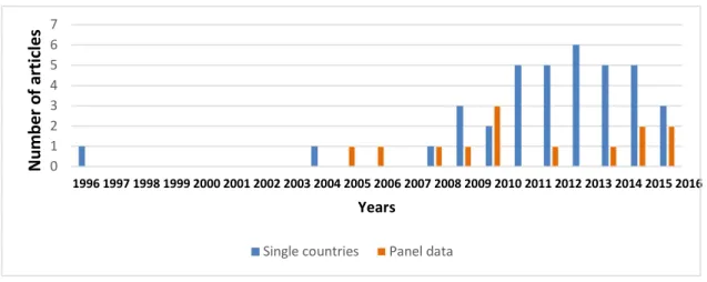
As shown in Figure 1, since the pioneer work of Ebohon (1996), a large body of economic literature has been published on the energy consumption-economic growth nexus in Sub-Saharan countries and has dramatically increased over time. However, the second study of the topic did not appear until 2004. The main reasons explaining the gap are the appearance of the new econometrics techniques later applied, and the availability of data used for Sub-Saharan countries. We identify 50 papers, including thirteen articles using econometric panel data analyses and thirty-seven using single-country time series.
14 Nevertheless, as shown in Figure 2, there is substantial heterogeneity among the results obtained by studies on the energy consumption-economic growth nexus for Sub-Saharan countries. As for developed countries, there is no consensus regarding the direction of causality for Sub-Saharan countries. But, the distribution of the lack of consensus among the studies appears more different than the other past studies on the field (Payne, 2010, p. 34-35).
Figure 2. Heterogeneity of results on the energy consumption-economic growth nexus
The studies use different sets of variables in order to explain energy consumption-economic growth nexus. The studies are classified into analytical categories of moderators, using binary variables (1 if the modality is true, 0 otherwise). These definitions, as well as descriptive statistics for all the variables included in our meta-analysis, are presented in Table 3.
Table 3. List of variables
0 1 2 3 4 5 6 7 1996 1997 1998 1999 2000 2001 2002 2003 2004 2005 2006 2007 2008 2009 2010 2011 2012 2013 2014 2015 2016 N um be r o f a rt ic le s Years
Single countries Panel data
H1 37% H2 11% H3 14% H4 38% Growth (H1) Conservation (H2) Bidirectional (H3) Neutrality (H4)
15
Variable Code Description Summary details
I. The characteristics of the study
Publication year yp Year of publication
Journal Classification rcnrs
=1 if published article, =0 if working paper
The classification of the journals is based on the French Centre National
de la Recherche Scientifique (CNRS) report
evaluation realized in 2015. All the articles published are ranked
Panel or time-series studies
pa =1 if panel data study, =0 if time-series study
Time span ts =0 if time span < 30 years, =1 if time span =30 years, =2 if time span > 30 years.
II. Country specifications
16 Benin Botswana Burkina Faso Burundi Cameroon Cape Verde Congo Central African Republic Chad Comoros Democratic Republic of the Congo Ivory Coast Djibouti Eritrea Ethiopia Gabon Gambia Ghana Guinea Guinea-Bissau Kenya Lesotho Liberia Madagascar Malawi Mali Mauritania Mauritius BN =1 if a country is represented, =0 otherwise 46 Sub-Saharan countries are referenced BA BF BI CN CV CO CE T CS RDC CI DJ EYE EE GN GE GA GEE GB KA LO LA MR MI MII ME MS
17 Mozambique Namibia Niger Nigeria Rwanda Sao Tomé & Principe Senegal Seychelles Sierra Leone South Africa Sudan Swaziland Tanzania Togo Uganda Zambia Zimbabwe MZE NE NR NA RA STP SL SS SLE SA SN SD TA TO UA ZA ZEE
III. Econometric methodologies
III.1. Unit root tests1
Augmented Dickey-Fuller (1979)
ADF =1 if ADF is applied, =0 otherwise
First generation
1 A unit root is defined as a stochastic trend in a time series (also called a “random walk with drift”). If a time series contains a unit root, it
means that the systematic pattern is unpredictable. Unit root tests are implemented to test the stationarity in a time series. The hypothesis is: “if a shift in time doesn’t cause a change in the shape of the distribution”.
The first generation tests have several limitations: [1] low power in small sample sizes; [2] unable to distinguish nonstationary series from stationary series; and are replaced by the second generation tests.
18 Philips-Peron (1987, 1988) PP =1 if PP is applied, =0 otherwise First generation Zivot-Andrews(1992) ZA =1 if ZA is applied, =0 otherwise First generation
Levin, Lin, & Chu (1992) LLC =1 if LLC is applied, = 0 otherwise
Second generation
Im, Pesaran, & Shin (1997)
IPS =1 if IPS is applied, =0 otherwise
Second generation
Maddala & Wu (1999) MW =1 if MW is applied,
=0 otherwise Second generation
Hadri (2000) H =1 if H is applied, =0 otherwise
Second generation
III.2. Cointegration tests2
Johansen & Juselius (1990)
JJ =1 if JJ is applied, =0 otherwise
First generation
2 The cointegration tests were introduced by Granger (1981). “An important property of I(1) variables is that a linear combination of these
two variables that is I(0) may exist. If this is the case, these variables are said to be cointegrated”.
The first generation tests have several limitations: [1] asymptotic properties and sensitive to specification errors in limited samples [2] it cannot identify the cointegrating vectors where there are multiple cointegrating relations [3] cannot be applied when one cointegrating vector of different orders exists; and are replaced by the second generation tests.
19 Gregory & Hansen (1996) GH =1 if GH is applied,
=0 otherwise
First generation
Autoregressive Distribution Lag (2001)
ARDL =1 if ARDL is applied, =0 otherwise
Second generation
Enders & Siklos (2001) EZ =1 if EZ is applied, =0 otherwise
III.3. Causality tests3
Granger causality (1969) GR =1 if GR is applied, = 0 otherwise
First generation
Toda and Yamamoto (1995)
GRY =1 if GRY is applied, = 0 otherwise
Second generation
3.4. Other econometric techniques
Bootstrap (1979) BS =1 if BS is applied, = 0 otherwise
A large number of samples is simulated and provides bootstrap test statistics as
well as bootstrap
3 The causality tests were introduced by Granger (1981). [1] The detects the structural changes in a variable that has a considerable impact
on another variable. [2] Two natures of causality are distinguished: long and short-run (a specific test is required to test the joint significance of the lagged explanatory variables by using an F-statistics or Wald test [3] causality test are often associated with the use of an error correction model (VCEM).
The first generation tests have several limitations: [1] It requires pre-testing cointegration before causality [2] it cannot be applied in the case of multivariate causality (impossible to identify the explanatory variable causing the causality through the error correction model; and are replaced by the second generation tests.
20
confidence intervals. Thus, researchers compare the
current test statistics to empirical distribution of the
bootstrap. The use of bootstrap econometric method is often associated
in finite samples with Monte-Carlo simulations
(Dwass, 1957). In some cases, under the null hypothesis the bootstrap statistics follow the same distribution as the actual test statistic under the null
hypothesis.
Monte-Carlo Simulations (1957)
MC =1 if MC are applied, = 0 otherwise
Study the small-sample properties of competing estimators for a given
estimating problem.
Provide “a thorough understanding of the repeated sample and sampling distribution concepts, which are crucial
21
to an understanding of econometrics”.
Modelling the data generation process and try to estimate the parameters of the model and statistical properties of estimators
Hodrick-Prescott (1997) HP =1 if HP filter is applied, =0 otherwise
Apply to remove trend movements and capture
structural breaks
Vector Error Correction
Model (1987) VCEM =1 if an VCEM is applied,
= 0 otherwise
Avoid pretesting procedure of the time series whether the variables are I(0) or I(1),
Detect several cointegrating relationships (variables are considered as endogenous)
Allow test procedure on the long-run
Generalized Moments
22
=0 otherwise Apply in the context of semiparametric models, where maximum likelihood
is not available
Pooled Mean Group PMG =1 if a PMG is applied, =0 otherwise
Apply to capture the dynamics on the sample by
allowing different lagged levels for the two variables tested (energy consumption and economic growth in our
model). By using instrumental variables, this
econometric technique deals with the endogeneity
of regressors. This method detects partial correlation between the explanatory variable and the error and solves the omitted dynamics
in statistic panel data models
Demand Model MAED =1 if a MAED is applied, =0 otherwise
Specific Model developed by the International Energy
23 IV. Energy consumption measurement indicators
Aggregated energy consumption
CET =1 if CET is used, =0 otherwise Diesel CD =1 if CD is used, =0 otherwise Oil CP =1 if CP is used, =0 otherwise Gas CG =1 if CG is used, =0 otherwise Coal CC =1 if CC is used, =0 otherwise Electricity CE =1 if CE is used, =0 otherwise Depends on countries natural dotation Kerosene CK =1 if CK is used, =0 otherwise Biofuels CB =1 if CB is used, =0 otherwise
24 Energy efficiency UE =1 if UE is used,
=0 otherwise
V. Control variables
Inflation rate TI =1 if TI is used, =0 otherwise
Unemployment rate TE =1 if TE is used, =0 otherwise
Capital formation FBCF =1 if FBCF is used, =0 otherwise
Urbanization rate FT =1 if FT is used, =0 otherwise
Oil prices PP =1 if PP are used, =0 otherwise
Bivariate / Multivariate
Level of CO2 emissions ECO2 =1 if ECO2 is used, =0 otherwise
Population rate P =1 if P is used, =0 otherwise
25 =0 otherwise Governmental expenditures DG =1 if DG are used, =0 otherwise
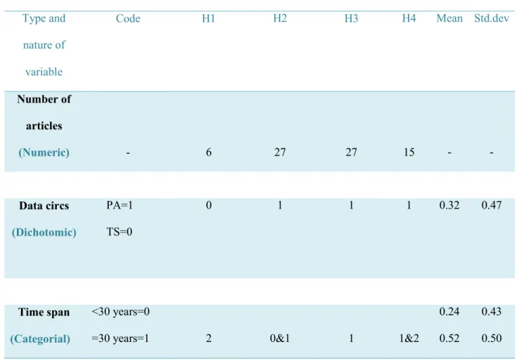
26 2.2. Descriptive statistics (Table 3.)
The results are grouped by hypothesis supported.
Table 4. Descriptive statistics
Type and nature of variable
Code H1 H2 H3 H4 Mean Std.dev
Number of articles (Numeric) - 6 27 27 15 - - Data circs (Dichotomic) PA=1 TS=0 0 1 1 1 0.32 0.47 Time span (Categorial) <30 years=0
=30 years=1 2 0&1 1 1&2
0.24 0.52
0.43 0.50
27 >30 years=2 0.24 0.43 Econometrics methods (Dichotomic) =1 GR =0 NO GR =1 GRY =0 GRNOY =1 GRVCEM =0GRNOVCEM 1 0 0 0 1 0 1 0 1 0 1 0 0.78 0.10 0.38 0.42 0.40 0.49 Energy consumption indicators (Dichotomic) =1 CET =0 NOCET =1 CE =0 NOCE =1 CP =0 NOCP =1 CD =0 NOCD =1 CG =0 NOCG 1 1 0 0 0 1 0 1 0 1 0 0 1 0 0 1 0 1 0 0 0.42 0.52 0.12 0.02 0.06 0.50 0.50 0.33 0.14 0.24
28 [1] The Growth hypothesis-based (H1) studies supporting unidirectional causality from energy consumption to economic growth are long-run time-series analyses that use the Granger causality test without an error correction model. Their models are based on univariate indicators as single aggregated energy consumption indicators or more specific indicators like electricity consumption by including control variables like inflation rate or CO2 emissions. This type of study is not representative in our sample because it concerns only six countries.
[2] The Conservation hypothesis-based (H2) studies validating unidirectional causality running from economic growth to energy consumption are medium-run panel data analyses that apply the Toda and Yamamoto causality procedure without error correction models. They use aggregated energy consumption or specified indicators (diesel consumption, gas consumption, coal consumption, or energy efficiency) and include control variables as proxies in a univariate framework. This type of study is representative in our sample because it concerns 27 countries. “The Conservation hypothesis” will be take as reference category for the multinomial logit model.
[3] The Feedback hypothesis-based (H3) studies that support bidirectional causality are both short-run and medium-short-run time-series analyses. These studies use Toda and Yamamoto causality procedure without error correction model. Aggregated energy consumption is excluded, and a multivariate framework is employed as specific indicators are used (oil consumption, coal consumption, and electricity consumption) without control variables. This type of study is representative in our sample because it concerns 27 countries
[4] The Neutrality hypothesis-based (H4) studies supporting the absence of causality are panel data analyses that use a bivariate model and specify energy consumption indicators in a multivariate
Models
(Dichotomic)
=1 Multivariate =0 Bivariate
29 framework (such as oil or gas consumption). This type of study is not representative in our sample because it only concerns 15 countries
30 For modeling the contribution of variables, two approaches are investigated: the first one, based on a Logit regression on each causality options, aims to identify what are the influent variables to each independent hypothesis. The second one, based on a Multinomial Logit Model, aims to establish a relation between hypothesis and identify the most explicative variables.
3.1. Logit on causality options with independent hypothesis
Implementing a qualitative econometric regression or using a binary variable is a major problem in econometrics (Cameron and Trivedi, 2010). Given a dependent variable coded Y, an appropriate choice of econometric model is necessary. If Y is a continuous variable, then it is appropriate for time-series or econometric panel data analyses to use the ordinary least squares with a best linear unbiased estimator (BLUE) that respects the Gauss-Markov assumptions (the model is well specified: E(ε) = 0; the errors are homoscedastic so the variance is constant equal to VAR(ε) = σ²; the error terms are uncorrelated each other cov(εt; εt’) = 0; and the errors are linearly independent of the exogenous variables with cov (ε;X) = 0). On the other hand, what if the dependent variable is a discrete random or unobserved variable? Three types of discrete random variables are identified in the econometric literature: the binary discrete random variable, ordered or unordered multiple discrete random variables, and accounting models. Our dependent variables fall under four hypotheses: H1, unidirectional causality running from energy consumption to economic growth, H2, unidirectional causality from economic growth to energy consumption, H3, bidirectional causality, and H4 neutrality. For each testable hypothesis, we can build econometric models; the final decision is linked to a sample of factors. We respect the general framework of probability models with Prob (event j occurs) = Prob (Y = j ) = F [parameters] as Y takes the value 0 with p probability and 1 with 1-p probability. The logit and probit models correspond to different regression models for p. The choice of adopting a logit or probit model is determined by the error charts (Chart 4) for each hypothesis (h1, h2, h3, h4), the minimization of the log-likelihood of each model, and the minimization of the Akaike information with AIC=-2LnL + 2k and the Schwartz criteria
31 as SC=-2LnL + KLnN. All this indicates that the null hypothesis of accepting the normal law is rejected. We use a logit model for each type of option. Those logit models are controlled by a contingency table in order to compare the observations and the predicted values to determine the concurring cases in the logit models.
3.2. Multinomial logit model (H2 is the reference category)
Multinomial logit model is implemented in order to establishing a relation between hypothesis and identifying the most explicative variables. This model is applied in response to the no significant results obtained for the logit models.
Multinomial choice implies a choice that provides the greatest utility among two or more alternatives;
Zij. zij includes both individual and choice characteristics. If we note z ij = [xij, wi] where xij represents the choice characteristics and wi the individual characteristics, in the case of a Multinomial Logit Model, the individual characteristics prevail on the choice characteristics (if the reverse is true, the conditional logit model is required). McFadden (1974) bases Multinomial Logit Model on the following test statistic,
Prob(Yi = j) = pij= exp(xiBj) / Σl=1m [exp(xiBj)], with the hypothesis j = 1 to m and where 0 < pij < 1 et Pml=1 [pij = 1)] (Cameron and Trivedi., 2010), if the J disturbances are independent and identically distributed with Gumbel (type 1 extreme value) distribution as: F(εij)= exp(-exp(-εij)).
For the causal relationships between gross domestic product (GDP) and energy consumption (EC), MNL is implemented on four directions of causality in an analysis of the 50 references about the Sub-Saharan countries. Each option chosen by a consumer is relative to the degree of utility it provides.
The utility for the four choices:
Ui1 = Pai1β1 + Ypi1β2 + Tsi1β3 +Gri1β4 +Gryi1β5 + Vcemi1β6 + α + γIi + εi1 (1)
32
Ui3 = Pai3β1 + Ypi3β2 + Tsi3β3 +Gri3β4 +Gryi3β5 + Vcemi3β6 + α + γIi + εi3 (3)
Ui4 = Pai4β1 + Ypi4β2 + Tsi4β3 +Gri4β4 +Gryi4β5 + Vcemi4β6 + α + γIi + εi4 (4)
Correspondingto the following matrix of attributes and characteristics:
4
34
4
4
4
Vcemi4
0
0
0
0
Ii
0
0
0
Vcemi3
3
3
3
3
3
0
1
0
Vcemi2
2
2
2
2
2
0
0
Ii
1
Vcemi1
1
1
1
1
1
Gryi
Gri
Tsi
Ypi
Pai
Gryi
Gri
Tsi
Ypi
Pai
Ii
Gryi
Gri
Tsi
Ypi
Pai
Gryi
Gri
Tsi
Ypi
Pai
Zi
MNL is primarily based on rejecting the hypothesis of independent irrelevant alternatives (IIA). This assumption supports the independence of log-odd ratios (Pij/Pim) relative to the remaining probabilities. Log-odd rations are described as the effects of one unit of change in X on the predicted odds ratio with other variables in the model held constant.
We apply MNL in our meta-analysis as follows:
Prob(Yi = j) = exp (z’ijθ)/ Σl=16 exp(z′ijθ) (1)
pij =exp Σexp
l=16
(xi11pa + xi22yp + xi33ts + xi44gr + xi55gry + xi66vcem)
(xi11pa + xi22yp + xi33ts + xi44gr + xi55gry + xi66vcem) (2)
33 pa: represents econometric panel data analysis;
yp: Publication year; ts: Time span;
gr: Granger causality test;
gry: Granger modified Toda and Yamamoto test; vcem: Error correction model.
Then, the calculation of marginal effects, based on the value of the parameters (the increase of one unit of a given estimator depends first on the value of other estimators and then on the starting value, meaning a difference between marginal effects and simple coefficients) helps identify the impact of significant variables on the assessment of each hypothesis. Three types of marginal effects are identified: the average marginal effect (AME), the marginal effect at mean (MEM), and the marginal effect at representative value (MER).
IV. EMPIRICAL RESULTS
Table 5. Logit on causality options
VARIABLES H1 H2 H3 H4
Panel Dataset (pa) 0.156 1.294 0.821 2.115
34 Publication Year (yp) 0.0390
(0.100) -0.0416 (0.157) -0.189 (0.144) -0.0626 (0.130) ** Time span (ht) -0.379 (0.550) 0.242 (0.727) 0.332 (0.539) 0.528 (0.675) Granger causality (gr) 1.057 (0.977) ** 0.133 (1.405) 0.0861 (1.058) -0.809 (1.071) Toda & Yamamoto
(gry) 0.284 (1.108) 3.459 (1.411) *** 0.786 (1.168) 1.556 (1.400) Error Correction Model (vcem) -1.781 (0.758) ** 1.409 (1.025) 1.814 (0.739) *** -0.0713 (0.853) Constant -78.68 (201.8) 80.27 (316 .2) 378.9 (229.3) 124.4 (262.2) Observations 50 50 50 50 Marginal Effects GR (+0.23 %) VCEM (-0.39 %) GRY (+0.69 %) VCEM (+0.42 %) AP (-0.04 %) PA (+0.45)
Standard errors in parentheses *** p<0.01, ** p<0.05, * p<0.1
35 Table 5 shows the significant variables identified for the logit model, corrected for heteroskedasticity. As indicated by the results of the residual forms of each causality option and the minimization of the Akaike and Schwartz criteria, we draw conclusions only from this model’s results. The logit of the first hypothesis (h1 or "Growth hypothesis") of unidirectional causality running from energy consumption to economic growth identifies two significant variables at close to 5 % (Student t-test for the coefficients): 4 the error correction model (VCEM) (P<0.05) and the use of the Granger causality test (gr)(P<0.05).
Looking at the marginal effects reveals that the use of the Granger causality test increases the probability of finding unidirectional causality running from energy consumption to economic growth by 0.23. In contrast, the use of an error correction model in the econometric analysis decreases the probability of asserting the "Growth hypothesis" by 0.39. For the "Conservation hypothesis" (h2), the logit model identifies only one significant variable: the use of the Toda and Yamamoto causality test. The use of the Toda and Yamamoto test increases by 0.69 the probability of supporting unidirectional causality running from economic growth to energy consumption. The logit model for "Feedback" (h3) identifies two significant variables: The error correction model (VCEM) (P<0.01) and the publication year (ap) (P<0.05). The use of the error correction model increases the probability of asserting the "Feedback" hypothesis by 0.42. On the other hand, the publication year decreases the probability of asserting the hypothesis by 0.04. The logit model for the "Neutrality” hypothesis (h4) admits only one variable: the use of an econometric panel data analysis, which increases by 0.45 the probability of supporting the "Neutrality hypothesis". The logit model is insufficient to inform on the nexus.
Thus, Multinomial Logit Model is implemented in order to establishing a relation between hypothesis and identifying the most explicative variables. The choose of H2 as the reference category is justified by two arguments: the first one is that the hypothesis is representative of the total sample. The second one is that this hypothesis concentrates more informations about the different level of integration of the non stationary variables.
4 The Student test tests if a given variable has an influence on the Y dependent variable. The null hypothesis is the H0=bj=0; otherwise the hypothesis is H1 = bj ≠ 0. Conserving the estimated coefficient and the standard deviation are necessary to compare the test statistic with t*. If t (absolute value) ≥ t*; we reject the null hypothesis of a significant variable.
36 Table 6. MNL reference categories: H2
(1) (1) (1)
VARIABLES
H1 H3 H4
37 (pa) (2.319) *** (2.490) (1.055) ** Publication Year (yp) -0.157 -0.108 -0.0554 (0.150) (0.389) (0.142) (0.534) Time span (ht) 1.783 (1.698) -0.223 0.534 (0.815) (0.839) Granger causality (gr) -18.21 -1.151 0.0289 (2.732) *** (2.439) (1.479)
Toda & Yamamoto (gry)
-2.471 -16.53 -0.959
(2.954) (1.378) *** (1.359)
Error Correction Model (vcem)
4.366 3.144 1.814
38 Observations 50 50 50 Marginal Effects PA (-0.53 %) VCEM (+ 0.16 %)
GRY
(+0.21 %) PA (+ 0.58 %)Standard errors in parentheses
*** p<0.01, ** p<0.05, * p<0.1
The empirical results of the multinomial logit model are displayed in Table 6 . The “Conservation” hypothesis is the reference category as [1] it is representative of the total sample and [2] it contains more information about the different integration levels of the non-stationary variables. For the following regressions, we create a hypo variable that takes the values h1, h2, h3, h4 by taking into account the causality results from our literature review. If the hypo takes the value h1 ("Growth hypothesis"), the use of econometric panel data analysis can be identified as a significant variable. As for the marginal effects, the use of econometric panel data analysis decreases the probability of asserting unidirectional
39 causality from energy consumption to economic growth by 0.53. If the hypo variable takes the value h3, two significant variables are presented: the error correction model (VCEM) and the use of the Toda and Yamamoto causality test (GRY). The use of the error correction model increases the probability of asserting the "Feedback" hypothesis by 0.16, whereas the use of a Toda and Yamamoto Causality test decreases the probability of asserting the "Feedback"' hypothesis by 0.21. If the hypo takes the h4 value, one significant variable is identified: econometric panel data analysis, which increases the probability of asserting the "Neutrality hypothesis" by 0.58.
V. CONCLUSION
In order to investigate the controversial issue of the relationship between economic growth and energy consumption for Sub-Saharan Africa, this contribution performs a meta-analysis, using 50 articles for the period 1996-2016, focusing on the main components of the literature studying the nexus. For modeling the contribution of variables, two methods are applied: First, in order to identify what are the influent variables to each independent hypothesis, a Logit regression on each causality options is applied. Second, in order to establish a relation between hypothesis and to identify the most explicative variables, a Multinomial Logit Model is implemented.
The findings are twofold. The first one is that logit model does not provide any useful information on causality options to determine what are the influent variables to each independant hypothesis. Logit regression is not significant to inform on the nexus.
The second one is that Multinomial Logit Model, implemented in order to establish a relation between hypothesis and identifying the most explicative variables, with the Conservation hypothesis as the reference category, shows that the panel variable is the most decisive one as it establishes a relation
40 between the hypothesis. This result provides interesting insights, for decision-makers and academics, to reinterpret the nexus for further energy policies implemented.
Nevertheless, any statistical inference of the results obtained by the investigation of the energy consumption-economic growth nexus for the Sub-Saharan countries should be interpreted with care. All studies are related to the specific context on Sub-Saharan countries. The economic growth and energy consumption measurement indicators are thus not constructed as well as they could be, and studies undertaken on the nexus suffer from potential estimation bias. Examples of mismeasurement include the proportion of the informal sector in economic activities in Africa, which is still substantial and thus difficult to capture in a single economic growth indicator. Similarly, when the electricity consumption indicator is employed, only a small part (reliant on traditional biomass) is captured in mainly grid-supplied demand.
APPENDICES
BIBLIOGRAPHY
META-ANALYSIS:
[1] Abedola. S.S., [2011], “Electricity Consumption and Economic Growth: Trivariate investigation in Botswana with Capital Formation”, International Journal of Energy Economics and Policy. Vol.1, No.2. [2] Adom. P.K., [2011], “Electricity Consumption-Economic Growth Nexus: The Ghanaian Case”. International Journal of Energy Economics and Policy, Vol.1, No.1, pp. 18-31.
[3] Akinlo. A.E., [2008]. “Energy consumption and economic growth: Evidence from 11 Sub-Sahara African Countries”, Energy Economics, Vol.30, pp. 2391-2400.
41 [4] Akinlo A.E. [2009]. “Electricity consumption and economic growth in Nigeria: Evidence from cointegration and co-feature analysis”. Journal of Policy Modeling, Vol. 2, pp. 244-263.
[5] Akomolafe A.K.J, Danladi J. [2014]. “Electricity Consumption and economic Growth in Nigeria: A Multivariate Investigation”. International Journal of Economics, Finance, and Management, Vol.3, No.4.
[6] Ali. H.S., Lwa. S.H., Yusop. Z., Chin. L., [2016]. “Dynamic implication of biomass energy consumption on economic growth in Sub-Saharan Africa: evidence from panel data analysis”. Forthcoming.
[7] Arimah. B.C., (1994). “Energy consumption and economic growth in Africa: a cross-sectional analysis” OPEC Review Summer, pp 207-221
[8] Asongu. S., El Montasser. G., Toumi. [2015]. “Testing the relationships between Energy Consumption, CO2 emissions and economic Growth in 24 countries: A Panel Approach” Working Paper, 10, 57-68.
[9] Bildirici. M.E., [2013]. “The analysis of the relationship between economic growth and electricity consumption in Africa by ARDL method, Energy Economics Letters, Vol.1, No.1, pp.1-14.
[10] Chontanawat. J., Hunt. L.C., & Pierse. R., [2006]. “Causality between energy consumption and GDP: evidence from 30 OECD and 78 non-OECD countries”, Surrey Energy Economics, Discussion Paper Series 113 University of Surrey, Guildford.
[11] Chontanawat. J., Hunt. L.C., & Pierse. R., [2008]. “Does energy consumption cause economic growth? Evidence from a systematic study of over 100 countries”. Journal of Policy Modeling, Vol. 30, pp. 209-20.
[12] Dlamini. J., Balcilar. M., Gupta. R., Inglesi-Lotz. R., [2002]. “Revisiting the causality between electricity consumption and economic growth in South Africa: a bootstrap rolling-window approach “. Economic Policy in Emerging Economies, Vol. 8, No.2.
42 [13] Dogan. E., [2014]. “Energy Consumption and Economic Growth: Evidence from Low-Income Countries in Sub-Saharan Africa”. International Journal of Energy Economics and Policy, Vol.4, No.2, pp.154-162.
[14] Ebohon O.J., [1996]. “Energy, economic growth and causality in developing countries: a case study of Tanzania and Nigeria”. Energy Policy, Vol.24, No.5, pp 447-453.
[15] Eggoh J.C., Bangake C., Rault C. [2011]. “Energy consumption and economic growth in African Countries”. Energy Policy, Vol.39, 7408-7421.
[16] Esso L.J. [2010]. “Threshold cointegration and causality relationship between energy use and growth in seven African countries”. Energy Economics, Vol.32, pp. 1383-1391.
[17] Farhani S., Ben Rejeb J. [2015]. “Link between Economic Growth and Energy Consumption in over 90 countries”. Working paper, (forthcoming).
[18] Grosset F., Nguyen-van P. [2015] Consommation d’énergie et croissance économique en Afrique Sub-saharienne, Working Paper.
[19] Iyke B.N. (2014), Electricity Consumption, Inflation, and Economic Growth in Nigeria: A Dynamic Causality Test, Working Paper (Forthcoming).
[20] Iyke B.N. (2015). “Electricity Consumption and economic growth in Nigeria: A revisit of the energy-growth debate. Energy Economics, Vol.51, pp. 166-176.
[21] Jumbe C.H.L. [2004]. “Cointegration and causality between electricity consumption and GDP: empirical evidence from Malawi”. Energy Economics, Vol.24, pp. 61-68.
[22] Kebede. E., Kagochi. J., Curtis M. Jolly. (2010). “Energy consumption and economic development in Sub-Sahara Africa”. Energy Economics, Vol.32, Issue.3, pp. 532-537.
[23] Kouakou A.K. (2011). “Economic growth and electricity consumption in Cote d’Ivoire: Evidence from time series analysis. Energy Policy, Vol.39, pp. 3638-3644.
43 [24] Kwakwa P.A. (2012). “Disaggregated Energy Consumption and Economic Growth in Ghana”. International Journal of Energy Economics and Policy, Vol.2, No.1.
[25] Kahsai M.S., Nondo C., Schaeer P.V., Gebremedhin T.G. [2012]. “Income level and the energy consumption-GDP nexus”: Evidence from Sub-Saharan Africa, Energy Economics, Vol.34, pp. 739-746.
[26] Lin B., Wesseh. Jr. P.K. (2014). “Energy consumption and economic growth in South Africa reexamined: A non-parametric testing approach”. Renewable and Sustainable Energy Reviews, Vol.40, pp. 840-850.
[27] Menyah K., Wolde-Rufael Y. [2010]. “Energy consumption, pollutant emissions and economic growth in South Africa. “Energy Economics, Vol.32, pp 1374-1382.
[28] Odhiambo N.M. (2009). “Electricity consumption and economic growth in South Africa: A trivariate causality test”. Energy Economics, Vol.31, pp. 635-640.
[29] Odhiambo N.M. (2009). “Energy consumption and economic growth nexus in Tanzania: An ARDL bounds testing approach”. Energy Policy, Vol.37, pp. 617-622.
[30] Odhiambo N.M. (2010). “Energy consumption, prices and economic growth in three SSA countries: A comparative study”. Energy policy, Vol.19, pp. 1-44.
[31] Ogundipe A.A., Akinyemi O., Ogundipe O.M. (2016). “Electricity consumption and Economic Development in Nigeria”. International Journal of Energy Economics and Policy, Vol.6 (1), pp. 134-143.
[32] Ogundipe A.A., Apata A. (2013). “Electricity consumption and Economic growth in Nigeria”. Journal of Business Management and Applied Economics, Vol.II, Issue 4.
[33] Okey M.K.N. (2009). “Energy consumption and GDP growth in WAEMU countries: A panel data analysis”. Working Paper
44 [34] Okoligwe N.E., Ihugba O.A. (2014). “Relationship between Electricity Consumption and Economic Growth: Evidence from Nigeria (1971-2012)”. Academic Journal of Interdisciplinary Studies, Vol.3, No.5. 14
[35] Olusegun A.A. (2008). “Energy consumption and economic growth in Nigeria: A Bounds Testing Cointegration Approach”. Journal of Economic Theory, Vol.2(4) : 118-123.
[36] Onakoya A.B., Onakoya A.O., Jimi-Salami O.A., Odedairo B.O. (2013). “Energy Consumption and Nigerian economic growth: an empirical analysis”. European Scientic Journal Vol.9, No.4.
[37] Onuanga S.M., (2012). “The relationship between commercial energy consumption and gross domestic income in Kenya’. The Journal of Developing Areas, Vol.46, No.1.
[38] Orhewhere B., Henry M., (2011). “Energy Consumption and Economic Growth in Nigeria”. JORIND (9) 1.
[39] Osigwe A.C., Arawomo D.F. (2015). “Energy Consumption, Energy Prices and Economic Growth: Causal Relationships Based on Error Correction Model”. International Journal of Energy Economics and Policy, Vol.5(2), pp. 408-414.
[40] Ouédraogo L.M. (2010). “Electricity consumption and economic growth in Burkina Faso: A cointegration analysis”, Energy Economics Vol.32, pp.524-531.
[41] Oyaromade R., Mathew A., Abalaba B.P. (2014). “Energy consumption and Economic Growth: A Causality Analysis”. Energy reports Vol. 1(2015), pp. 62-70.
[42] Solarin S.A., Shahbaz M. [2013]. “Trivariate Causality between Economic Growth, Urbanization, and Electricity Consumption in Angola: Cointegration and Causality Analysis”. Working Paper
[43] Tamba J.G, Njomo D., Limanond T., Ntsafack B. [2012]. “Causality analysis of diesel consumption and economic growth in Cameroon”. Energy Policy, Vol. 45, pp. 567-575.
[44] Wandji Y.D.F. (2015). “Energy consumption and economic growth: Evidence from Cameroon”. Energy Policy, Vol.61, pp. 1295-1304.
45 [45] Wessey Jr. P.K., Zoumara B. (2012).” Causal independence between energy consumption and economic growth in Liberia: Evidence from a non-parametric bootstrapped causality test”. Energy Policy, Vol.50, pp. 518-527.
[46] Wolde E.T., Mulugeta W., Hussen M.M. (2016). “Energy Consumption, Carbon Dioxide Emissions and economic growth in Ethiopia”. Global Journal of Management and Business Research:B Economics and commerce Vol.16, Issue 2.
[47] Wolde-Rufael Y. (2005). “Energy demand and economic growth: The African experience”. Journal of policy Modeling, Vol. 27, pp. 891-903.
[48] Wolde-Rufael Y. (2006). “Electricity consumption and economic growth: a time series experience for 17 African countries”. Energy Policy, Vol. 34, pp. 1106-1114.
[49] Zarnikau, J. (1996). “A reexamination of the causal relationship between energy consumption and gross national product”. Journal of Energy and Development, Vol. 21, pp. 229-239.
[50] Zerbo, E. [1996] CO2 emissions, growth, energy consumption and foreign trade in Sub-Saharan African Countries, Working Paper.
OTHER:
[1] Abosedra. S., & Baghestani. H., [1991], “New evidence on the causal relationship between United States energy consumption and gross national product”, Journal of Energy and Development, 30 (2), 123-162. Vol. 14, pp. 285-92.
[2] Akarca. A.T., & Long. T.V., [1979], “Energy and employment: a time series analysis of the causal relationship”. Resources and Energy. Vol. 2, pp. 151-62.
46 [3] Akarca. A.T. & Long, T.V. [1980]. “On the relationship between energy and GNP: a reexamination”. Journal of Energy and Development, Vol. 5, pp. 326-31.
[4] Alinsato. A.S., [2013]. “Electricity Consumption and Gross domestic product in an electricity community: Evidence from bound testing cointegration and Granger-causality tests”. Journal of Economics and International Finance, Vol. 5(4), pp. 99-105.
[5] Bowden. N., & Payne. J.E., [2008]. “Sectoral analysis of the causal relationship between renewable and non-renewable energy consumption and real output in the US Energy Sources, Part B: Economics, Planning, and Policy” (forthcoming).
[6] Cameron A.C., Trivedi P.K. [2010]. “Microeconometrics using stata”, A Stata Press Publication, Stata Corp LP, College station, Texas.
[7] Cheng, B.S. [1996]. “An investigation of cointegration and causality between energy consumption and economic growth”. Journal of Energy and Development, Vol. 21, pp. 73-84.
[8] Climent. F., & Pardo. A., [2007]. “Decoupling factors on the energy-output linkage: The Spanish case “Energy Policy, Vol. 35, pp. 522-8.
[9] Cogley. T., & Nason. J.M., (1995). “Effects of the Hodrick-Prescott filter on trend and difference stationary time series Implications for business cycle research”. Journal of Economic Dynamics & Control, vol.19, pp. 253-278.
[10] Davidson. R., & MacKinnon. J.G., (2005). “Bootstrap Methods in Econometrics”.
[11] Efron. B., (1979). “Bootstrap methods”. Another look at jackknife. Ann. Stat, vol.7, pp. 1-26. [12] Engle. R.F., & Granger. W.J., (1987). “Co-integration and Error Correction: Representation, Estimation, and Testing”. Econometrica, Vol. 55, n°2, pp. 251-276.
[13] Erol, U. and Yu, E.S.H. [1987b]. “Time series analysis of the causal relationships between US energy and employment”. Resources and Energy, Vol. 9, pp. 75-89.
47 [14] Erol, U. and Yu, E.S.H. [1989]. “Spectral analysis of the relationship between energy consumption, employment and business cycles”. Resources and Energy, Vol. 11, pp. 395-412.
[15] Frisch R., (1933). “Editor’s note”. Econometrica, 1, 1-4.
[16] Glasure, Y.U. and Lee, A.R. [1995]. “Relationship between US energy consumption and employment: further evidence. “Energy Sources, Vol. 17, pp. 509-16.
[17] Glasure, Y.U. and Lee, A.R. [1996]. “The macroeconomic effects of relative prices, money and federal spending on the relationship between US energy consumption and employment”. Journal of Energy and Development, Vol. 22, pp. 81-91.
[18] Granger. C., (1986). “Forecasting Economic Time Series”. Academic Press, 2nd edition. [19] Gregory. A.W., Nason. J.M., Watt. D.G., (1996). “Testing for structural breaks in cointegrated relationships”. Journal of Econometrics, vol.71, pp 321-341.
[20] Gregory. A.W., Hansen. B.E., (1996). “Tests for Cointegration in Models with Regime and Trend Shifts”. Oxford Bulletin of Economics and Statistics, vol. 58 (3), pp 0305-9049.
[21] Hadri. K., (2000). “Testing for stationarity in heterogeneous panel data”. Econometrics Journal, Vol.3, pp. 148-161.
[22] Hamilton. J.D., (1994). “Time Series Analysis”. Princeton University Press, Princeton, NJ.
[23] Hodrick. R.J. & Prescott. E.C., (1980). “Postwar U.S Business Cycles: An Empirical Investigation”. Canergie Melton University, discussion paper n°451.
[24] Hodrick. R.J., & Prescott. E.C., (1997). “Postwar U.S. Business Cycles: An Empirical Investigation”. Journal of Money, Credit and Banking, vol 29:1, pp. 1-16.
[25] Hsiao. C., (1979). “Causality tests in Econometrics”. Journal of Economic Dynamics and Control, pp 321-346.
48 [27] Im. K.S., Pesaran. M.H., Shin. Y., (2003). “Testing for unit roots in heterogeneous panels”. Journal of Econometrics, Vol 115, pp 53-74.
[28] Johansen. S., (1995). “Likelihood-based inference in cointegrated vector autoregressive models, Oxford University Press, Oxford.
[29] Karanfil. F., (2008). “Energy consumption and economic growth revisited: does the size of unrecorded economy matter?”. Energy Policy, Vol. 36, pp 3019-3025.
[30] Karanfil. F., (2009). “How many times again will we examine the energy-income nexus using a limited range of traditional econometric tools”. Energy Policy, Vol. 37, pp 1191-1194.
[31] Karanfil F., Li Y. (2015). “Electricity consumption and economic growth: Exploring panel specific differences. Energy Policy, Vol.82, pp. 264-277.
[32] Maddala. G.S., Wu. S., (1999). “A comparative study of unit root tests with panel data and a new simple test. Oxford Bulletin of economics and statistics, special issue n° 0305-9049.
[33] Nkoro. E., & Uko. A.K., (2016). “Autogressive Distributed Lag (ARDL) cointegration technique: application and interpretation”. Journal of Statistical and Econometric Methods, vol.5, n°4, pp 63-91. [34] Pesaran. M.H. & Shin. Y., (1999). “An Autoregressive Distributed Lag Modeling Approach to Cointegration Analysis”. Cambridge University Press, Cambridge.
[35] Pesaran. M.H., Smith. R., Shin. Y., (2001). “Bounds Testing Approaches to the Analysis of Level Relationships”. Journal of Applied Econometrics, vol. 16, pp 289-326.
[36] Phillips. P., & Perron. P., (1988). “Testing for a Unit root in Time Series Regression”. Bimetrika, vol.75, pp 335-346.
[37] Sims., C (1972). “Money, Income and Causality”. American Economic Review, vol.62, pp 540-552.
49 [38] Toda. H., Yamamoto. T., (1995). “Statistical inference in vector autoregressions with possibly integrated processes”. Journal of Econometrics, vol. 66, 1-2, pp. 225-250.
[39] Zarnikau, J. (1996). “A reexamination of the causal relationship between energy consumption and gross national product”. Journal of Energy and Development, Vol. 21, pp. 229-239.