Quantum transport in gated dangling-bond atomic wires

Supporting Information: Quantum transport

in gated dangling-bond atomic wires

S. Bohloul,

_{Q. Shi,}

_{Robert A. Wolkow,}

_{and Hong Guo}

†Center for the Physics of Materials and Department of Physics, McGill University,

Montreal, Quebec H3A 2T8, Canada

‡National Institute for Nanotechnology, National Research Council of Canada, Edmonton,

Alberta, Canada T6G 2M9

¶Department of Physics, University of Alberta, Edmonton, Alberta, Canada T6G 2E1

E-mail: saeed.bohloul@mail.mcgill.ca

Atomic sphere approximation

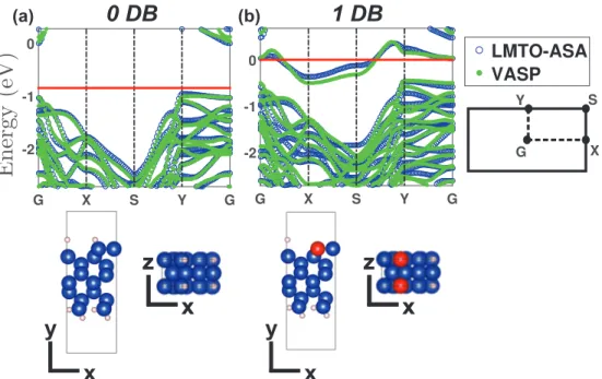
In this section, we present details of the atomic sphere approximation (ASA) used in our transport calculations. Figure S1(a) shows electronics structure of a fully passivated Si(100)-2x1:H (0DB) and Figure S1(b) corresponds to a Si(100)-Si(100)-2x1:H surface hosting one DB (1DB). Closeness of bands in vicinity of the Fermi level as compared with those from VASP conrms the appropriateness of adopted ASAs for subsequent zero bias transport calculations. The corresponding ASA parameters, namely radii and positions of atomic spheres, are given in Tables S1, S2, S3. These two systems are the building blocks for constructing subsequent two-probe structures.

(a)

0 DB

1 DB

y

x

z

x

z

x

y

x

z

x

z

x

Figure S1: Comparison of electronic band structure near the Fermi level (the red line) calcu-lated by VASP (green-lled circles) and LMTO-ASA (blue-unlled circles), for (a) Si(100)-2x1:H surface without any DB (0DB), (b) Si(100)-Si(100)-2x1:H surface with an unsaturated DB (1DB). The bands agreement veries the accuracy of ASA scheme. Top and side view of each structure is shown in bottom panels. Blue and white atoms represent Si and H, respectively, while a DB is shown by red.

Tight-binding calculations

In order to further demonstrate the nature of the gating mechanism, we simulated DBC-DBW systems by a tight binding model at the single-orbital nearest-neighbour level. The Hamiltonian of the system can be written as

Hsys = ∑ ϵia†iai+ ∑ ti,i+1a†iai+1+h.c.+ ∑ hmc†mcm+ ∑ pmic†mai+h.c.+ ∑ hmnc†mcn+h.c.,

Single-gated wire: ϵi =−0.03eV, ti,i+1 = 0.1eV, hm = 0eV, pmi = 0.03eV,

Uncoupled double-gated wire: ϵi =−0.03eV, ti,i+1 = 0.1eV, hmgate1 = 0eV,hmgate2 = 0eV,

pmi= 0.03eV, hmn = 0eV,

Coupled double-gated wire: ϵi = −0.03eV, ti,i+1 = 0.1eV, hmgate1 = 0eV,hmgate2 =

−0.05eV, pmi= 0.03eV, hmn= 0.11eV.

As can be seen, in case of coupled double-gated wire, on-site energies of DBCs are split-ted by ∼ 0.05eV which predicts an interaction potential of ∼ 0.10eV between the gates. Once appropriate parameters are chosen, the transmission coecient is calculated by NEGF formalism, as shown in Figure (4) of the main text.

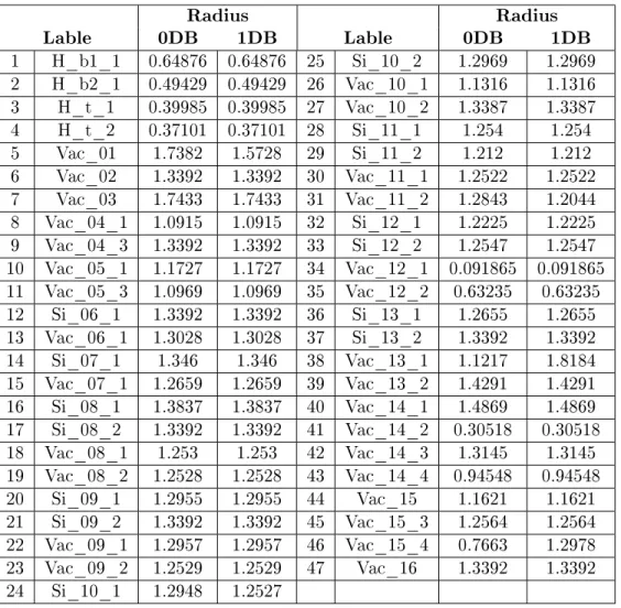
Table S1: Radius of various atomic spheres used in the ASA of 0DB and 1DB systems. For each sphere, the rst part of the label indicates corresponding chemical element. All units are in angstroms. Radius Radius Lable 0DB 1DB Lable 0DB 1DB 1 H_b1_1 0.64876 0.64876 25 Si_10_2 1.2969 1.2969 2 H_b2_1 0.49429 0.49429 26 Vac_10_1 1.1316 1.1316 3 H_t_1 0.39985 0.39985 27 Vac_10_2 1.3387 1.3387 4 H_t_2 0.37101 0.37101 28 Si_11_1 1.254 1.254 5 Vac_01 1.7382 1.5728 29 Si_11_2 1.212 1.212 6 Vac_02 1.3392 1.3392 30 Vac_11_1 1.2522 1.2522 7 Vac_03 1.7433 1.7433 31 Vac_11_2 1.2843 1.2044 8 Vac_04_1 1.0915 1.0915 32 Si_12_1 1.2225 1.2225 9 Vac_04_3 1.3392 1.3392 33 Si_12_2 1.2547 1.2547 10 Vac_05_1 1.1727 1.1727 34 Vac_12_1 0.091865 0.091865 11 Vac_05_3 1.0969 1.0969 35 Vac_12_2 0.63235 0.63235 12 Si_06_1 1.3392 1.3392 36 Si_13_1 1.2655 1.2655 13 Vac_06_1 1.3028 1.3028 37 Si_13_2 1.3392 1.3392 14 Si_07_1 1.346 1.346 38 Vac_13_1 1.1217 1.8184 15 Vac_07_1 1.2659 1.2659 39 Vac_13_2 1.4291 1.4291 16 Si_08_1 1.3837 1.3837 40 Vac_14_1 1.4869 1.4869 17 Si_08_2 1.3392 1.3392 41 Vac_14_2 0.30518 0.30518 18 Vac_08_1 1.253 1.253 42 Vac_14_3 1.3145 1.3145 19 Vac_08_2 1.2528 1.2528 43 Vac_14_4 0.94548 0.94548 20 Si_09_1 1.2955 1.2955 44 Vac_15 1.1621 1.1621 21 Si_09_2 1.3392 1.3392 45 Vac_15_3 1.2564 1.2564

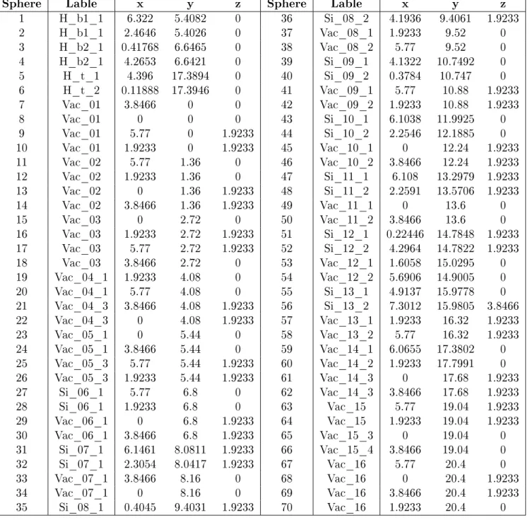
Table S2: Coordinates and type of atomic sites used in the ASA of Si(100)-2x1:H without any DB (0DB). The unit-cell is dened by ⃗a = (7.6933, 0, 0), ⃗b = (0, 21.7600, 0), and ⃗c = (0, 0, 3.8466). All lengths are in angstroms.

Sphere Lable x y z Sphere Lable x y z

1 H_b1_1 6.322 5.4082 0 36 Si_08_2 4.1936 9.4061 1.9233 2 H_b1_1 2.4646 5.4026 0 37 Vac_08_1 1.9233 9.52 0 3 H_b2_1 0.41768 6.6465 0 38 Vac_08_2 5.77 9.52 0 4 H_b2_1 4.2653 6.6421 0 39 Si_09_1 4.1322 10.7492 0 5 H_t_1 4.396 17.3894 0 40 Si_09_2 0.3784 10.747 0 6 H_t_2 0.11888 17.3946 0 41 Vac_09_1 5.77 10.88 1.9233 7 Vac_01 3.8466 0 0 42 Vac_09_2 1.9233 10.88 1.9233 8 Vac_01 0 0 0 43 Si_10_1 6.1038 11.9925 0 9 Vac_01 5.77 0 1.9233 44 Si_10_2 2.2546 12.1885 0 10 Vac_01 1.9233 0 1.9233 45 Vac_10_1 0 12.24 1.9233 11 Vac_02 5.77 1.36 0 46 Vac_10_2 3.8466 12.24 1.9233 12 Vac_02 1.9233 1.36 0 47 Si_11_1 6.108 13.2979 1.9233 13 Vac_02 0 1.36 1.9233 48 Si_11_2 2.2591 13.5706 1.9233 14 Vac_02 3.8466 1.36 1.9233 49 Vac_11_1 0 13.6 0 15 Vac_03 0 2.72 0 50 Vac_11_2 3.8466 13.6 0 16 Vac_03 1.9233 2.72 1.9233 51 Si_12_1 0.22446 14.7848 1.9233 17 Vac_03 5.77 2.72 1.9233 52 Si_12_2 4.2964 14.7822 1.9233 18 Vac_03 3.8466 2.72 0 53 Vac_12_1 1.6058 15.0295 0 19 Vac_04_1 1.9233 4.08 0 54 Vac_12_2 5.6906 14.9005 0 20 Vac_04_1 5.77 4.08 0 55 Si_13_1 4.9137 15.9778 0 21 Vac_04_3 3.8466 4.08 1.9233 56 Si_13_2 7.3012 15.9805 3.8466 22 Vac_04_3 0 4.08 1.9233 57 Vac_13_1 1.9233 16.32 1.9233 23 Vac_05_1 0 5.44 0 58 Vac_13_2 5.77 16.32 1.9233 24 Vac_05_1 3.8466 5.44 0 59 Vac_14_1 6.0655 17.3802 0 25 Vac_05_3 5.77 5.44 1.9233 60 Vac_14_2 1.9233 17.7991 0 26 Vac_05_3 1.9233 5.44 1.9233 61 Vac_14_3 0 17.68 1.9233 27 Si_06_1 5.77 6.8 0 62 Vac_14_3 3.8466 17.68 1.9233 28 Si_06_1 1.9233 6.8 0 63 Vac_15 5.77 19.04 1.9233 29 Vac_06_1 0 6.8 1.9233 64 Vac_15 1.9233 19.04 1.9233 30 Vac_06_1 3.8466 6.8 1.9233 65 Vac_15_3 0 19.04 0 31 Si_07_1 6.1461 8.0811 1.9233 66 Vac_15_4 3.8466 19.04 0 32 Si_07_1 2.3054 8.0417 1.9233 67 Vac_16 5.77 20.4 0 33 Vac_07_1 3.8466 8.16 0 68 Vac_16 0 20.4 1.9233 34 Vac_07_1 0 8.16 0 69 Vac_16 3.8466 20.4 1.9233 35 Si_08_1 0.4045 9.4031 1.9233 70 Vac_16 1.9233 20.4 0

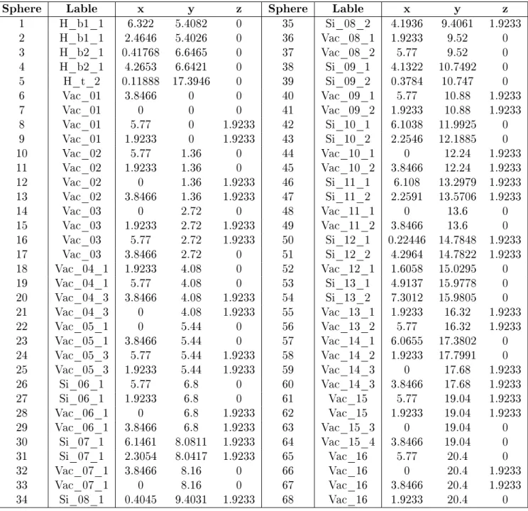
Table S3: Coordinates and type of atomic sites used in the ASA of Si(100)-2x1:H with one DB (1DB). The unit-cell is dened by ⃗a = (7.6933, 0, 0), ⃗b = (0, 21.7600, 0), and ⃗c = (0, 0, 3.8466). All lengths are in angstroms.

Sphere Lable x y z Sphere Lable x y z

1 H_b1_1 6.322 5.4082 0 35 Si_08_2 4.1936 9.4061 1.9233 2 H_b1_1 2.4646 5.4026 0 36 Vac_08_1 1.9233 9.52 0 3 H_b2_1 0.41768 6.6465 0 37 Vac_08_2 5.77 9.52 0 4 H_b2_1 4.2653 6.6421 0 38 Si_09_1 4.1322 10.7492 0 5 H_t_2 0.11888 17.3946 0 39 Si_09_2 0.3784 10.747 0 6 Vac_01 3.8466 0 0 40 Vac_09_1 5.77 10.88 1.9233 7 Vac_01 0 0 0 41 Vac_09_2 1.9233 10.88 1.9233 8 Vac_01 5.77 0 1.9233 42 Si_10_1 6.1038 11.9925 0 9 Vac_01 1.9233 0 1.9233 43 Si_10_2 2.2546 12.1885 0 10 Vac_02 5.77 1.36 0 44 Vac_10_1 0 12.24 1.9233 11 Vac_02 1.9233 1.36 0 45 Vac_10_2 3.8466 12.24 1.9233 12 Vac_02 0 1.36 1.9233 46 Si_11_1 6.108 13.2979 1.9233 13 Vac_02 3.8466 1.36 1.9233 47 Si_11_2 2.2591 13.5706 1.9233 14 Vac_03 0 2.72 0 48 Vac_11_1 0 13.6 0 15 Vac_03 1.9233 2.72 1.9233 49 Vac_11_2 3.8466 13.6 0 16 Vac_03 5.77 2.72 1.9233 50 Si_12_1 0.22446 14.7848 1.9233 17 Vac_03 3.8466 2.72 0 51 Si_12_2 4.2964 14.7822 1.9233 18 Vac_04_1 1.9233 4.08 0 52 Vac_12_1 1.6058 15.0295 0 19 Vac_04_1 5.77 4.08 0 53 Si_13_1 4.9137 15.9778 0 20 Vac_04_3 3.8466 4.08 1.9233 54 Si_13_2 7.3012 15.9805 0 21 Vac_04_3 0 4.08 1.9233 55 Vac_13_1 1.9233 16.32 1.9233 22 Vac_05_1 0 5.44 0 56 Vac_13_2 5.77 16.32 1.9233 23 Vac_05_1 3.8466 5.44 0 57 Vac_14_1 6.0655 17.3802 0 24 Vac_05_3 5.77 5.44 1.9233 58 Vac_14_2 1.9233 17.7991 0 25 Vac_05_3 1.9233 5.44 1.9233 59 Vac_14_3 0 17.68 1.9233 26 Si_06_1 5.77 6.8 0 60 Vac_14_3 3.8466 17.68 1.9233 27 Si_06_1 1.9233 6.8 0 61 Vac_15 5.77 19.04 1.9233