Semiquantitation of paralytic shellfish toxins by hydrophilic interaction liquid chromatography-mass spectrometry using relative molar response factors

Supplementary Materials: Semiquantitation of

Paralytic Shellfish Toxins by Hydrophilic Interaction

Liquid Chromatography-Mass Spectrometry Using

Relative Molar Response Factors

Jiangbing Qiu, Elliott J. Wright, Krista Thomas, Aifeng Li, Pearse McCarron and Daniel G. Beach

Figure S1. A flow diagram of M-toxins semipurification.

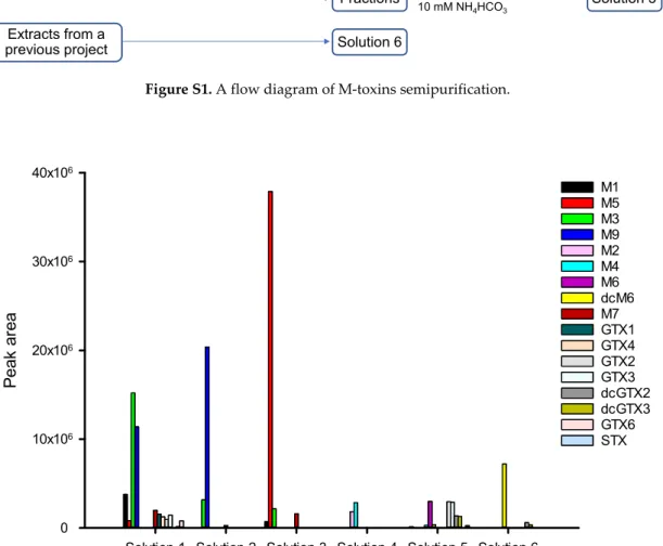
Figure S2. LC-MS/MS (ESI+_{) Peak areas of M-toxins and other PST analogues in mixed solutions of} semi-purified fractions. Extracts of laboratory-exposed mussel Solution 1 Solution 2 1.5 cm ID × 115 cm Bio-Gel P-2 0.1 M HAc Extracts from a

previous project Solution 3

1.5 cm ID × 115 cm Bio-Gel P-2 0.1 M HAc Extracts of field collected mussel Solution 4 Fractions 1.5 cm ID × 170 cm Bio-Gel P-2 0.1 M HAc Solution 5 1.5 cm ID × 170 cm Bio-Gel P-2 10 mM NH4HCO3 Solution 6 Extracts from a previous project

Solution 1 Solution 2 Solution 3 Solution 4 Solution 5 Solution 6

Pe

ak

a

re

a

Toxins 2020, 12, x; doi: S2 of S4

Figure S3. Product ion spectra of M-toxins collected from HILIC-CAD-MS/MS runs of semi-purified

fractions. M1 at m/z 396 (A), M2 at m/z 316 (B), M3 at m/z 412 (C), M4 at m/z 332 (D), M5 at m/z 396 (E), M6 at m/z 316 (F), dcM6 at m/z 273 (G) and M9 at m/z 428 (H). 50 100 150 200 250 300 350 400 R el at iv e Abu nd an ce 0 20 40 60 80 100 378.1 316.1 298.1 273.1 M1 50 100 150 200 250 300 350 400 0 20 40 60 80 100 298.1 257.1 237.1 148.0 220.1 196.1 282.1 M2 50 100 150 200 250 300 350 400 450 R el at iv e A bu ndan ce 0 20 40 60 80 100 394.1 332.1 314.1 289.1 M3 50 100 150 200 250 300 350 400 0 20 40 60 80 100 314.1 296.1 164.0 M4 50 100 150 200 250 300 350 400 R el at iv e A bu nd an ce 0 20 40 60 80 100 316.1 378.1 298.1 273.1 257.1 M5 50 100 150 200 250 300 350 400 0 20 40 60 80 100 257.1 298.1 239.1 148.0 M6 m/z 50 100 150 200 250 300 350 400 R el at iv e A bu ndan ce 0 20 40 60 80 100 214.1 255.1 196.1 273.1 dcM6 m/z 100 150 200 250 300 350 400 450 0 20 40 60 80 100 428.1 348.1 330.1 M9

A

H

G

F

E

D

C

B

Toxins 2020, 12, x; doi: S3 of S4

Table S1. Calibration data for PST CRM calibration solutions by HILIC-CAD. Solution Charge State PST range (ng on column) Linear regression

Equation R2 neutrala C1 14–216 y = 0.53x + 2.40 0.9971 C2 9.1–73 y = 0.51x + 0.37 0.9993 +1a GTX1 26–183 y = 0.68x + 1.92 0.9991 GTX4 9.4–66 y = 0.59x - 0.03 0.9984 GTX2 13–151 y = 0.65x - 0.28 0.9992 GTX3 5.5–66 y = 0.60x + 0.26 0.9983 GTX5 12–95 y = 0.64x + 3.33 0.9957 GTX6 17–55 y = 0.62x + 0.88 0.9962 dcGTX2 20–199 y = 0.65x + 2.46 0.9982 dcGTX3 6.8–68 y = 0.72x - 0.17 0.9994 +2b STX 6.5–78 y = 0.73x + 0.56 0.9993 NEO 13–106 y = 0.74x + 3.04 0.9991 dcNEO 11–55 y = 0.71x + 2.85 0.9973 dcSTX 11–91 y = 0.75x + 2.61 0.9997

a _{analyzed using gradient 1.} b _{analyzed using gradient 2.}

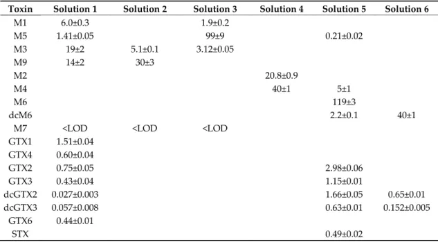
Table S2. Concentration of PST analogues in mixed standards solutions of combined fractions (μM)

as determined by HILIC-CAD. Uncertainties indicate standard deviation of triplicate injections.

Toxin Solution 1 Solution 2 Solution 3 Solution 4 Solution 5 Solution 6

M1 6.0±0.3 1.9±0.2 M5 1.41±0.05 99±9 0.21±0.02 M3 19±2 5.1±0.1 3.12±0.05 M9 14±2 30±3 M2 20.8±0.9 M4 40±1 5±1 M6 119±3 dcM6 2.2±0.1 40±1

M7 <LOD <LOD <LOD

GTX1 1.51±0.04 GTX4 0.60±0.04 GTX2 0.75±0.05 2.98±0.06 GTX3 0.43±0.04 1.15±0.01 dcGTX2 0.027±0.003 1.66±0.05 0.65±0.01 dcGTX3 0.057±0.008 0.63±0.01 0.152±0.005 GTX6 0.44±0.01 STX 0.49±0.02

Table S3. Gradient elution methods and corresponding reverse gradients in LC-CAD-MS. Gradient Method Time (min) A (%) B (%)

1 Analytical gradient 0 10 90 15 45 55 50 45 55 50 10 90 75 10 90

Reverse gradient for compensation 0 90 10 4.5 90 10 19.5 55 45 54.5 55 45 55 90 10 75 90 10

Toxins 2020, 12, x; doi: S4 of S4 2 Analytical gradient 0 10 90 25 45 55 27 70 30 40 70 30 40 10 90 60 10 90

Reverse gradient for compensation 0 90 10 5.8 90 10 30.8 55 45 32.8 30 70 45.8 30 10 45.8 90 10 60 90 10