Analytical study and cost modeling of secondary aluminum consumption for alloy producers under uncertain demands

Analytical Study and Cost Modeling of Secondary Aluminum

Consumption for Alloy Producers under Uncertain Demands

by Yaoqi Li

B.S. Optical Information Science and Technology, Fudan University, 2006 B.Eng. Material Science and Engineering, University of Birmingham, 2006

Submitted to the Department of Materials Science and Engineering in Partial Fulfillment of the Requirements for the Degree of

Master of Science in Materials Science and Engineering Massachusetts Institute of Technology

June 2008

@2008 Massachusetts Institute of Technology. All rights reserved.

MASSACHUSETTS INSTITUTE

OF TECHNOLOGY

JUN 16 2008

LIBRARIES

Signature of Author _{... .... .}

Dpartment oMaterials SciencV and Engineering and 23 May 2008

Certified by ... ... . ... ... ..

/

-Randolph

Kirchain

Assistant Professor of Materials Science and Engineering and Engineering Systems Division Thesis Supervisor

Accepted by ... ...

Samuel M. Allen Professor of Materials Science and Engineering Chair, Departmental Committee on Graduate Students

Analytical Study and Cost Modeling of Secondary Aluminum

Consumption for Alloy Producers under Uncertain Demands

by Yaoqi Li

Submitted to the Department of Materials Science and Engineering on 23 May 2008 in Partial Fulfillment of the Requirements for

the Degree of Master of Science in Materials Science and Engineering

Abstract

A series of case studies on raw materials inventory strategy for both wrought and cast aluminum alloy productions were conducted under recourse-based modeling framework with the explicit considerations of the demand uncertainty compared to the traditional strategy based on point forecast of future demand. The result shows significant economic and environmental benefits by pre-purchasing excess amount of cheaper but dirtier secondary raw materials to hedge the riskier higher-than-expected demand scenario. Further observations demonstrate that factors such as salvage value of residual scraps, cost advantage of secondary materials over primary materials, the degree of the demand uncertainty, etc. all have direct impacts on the hedging behavior. An analytical study on a simplified case scenario suggested a close form expression to well explain the hedging behavior and the impacts of various factors observed in case studies.

The thesis then explored the effects of commonality shared by secondary materials in their application in multiple final products. Four propositions were reached.

Thesis Supervisor: Randolph Kirchain

Acknowledgement

Time at Materials System Laboratory (MSL) will be one of the most memorable ones in my life.

I feel extremely fortunate to have Professor Randolph Kirchain as my research advisor. During the course of my graduate research, Professor Kirchain is always ready to spend his valuable time with me in discussing any problems I met during my research. He always promptly and responsively advises me by emailing me even though it might be late night or during the weekends. Even when his schedule becomes extremely tight, he still spends his out-of-office time to give very detailed comments on my thesis paragraph by paragraph. Under his advisory, I not only learn research skills from him, but more importantly I also try to learn his hard working ethics, excellent problem solving skills, kindness towards people around him, the sense of humor towards any academic problems. All these qualities will definitely benefit my whole career in the future.

I am also very thankful to Dr. Richard Roth, Dr. Frank Field and Terra Cholfin who helped me generously along my journey with MSL. I still remember it was a hard decision to make one year ago to bring me into the MSL community considering the almost saturated group size. Without the Rich and Randy's confidence in me, I will not get the opportunity to work in MSL.

Equally important, without tremendous help from the whole MSL community, my research cannot go anywhere. Especially, I really appreciate continuous advice from Gabby, valuable suggestions from Elisa, help from Elsa on a daily basis and so on. Supports and friendship from other MSL members, Jeff, Catarina, Tommy, Jeremy, Jonahtan, Shan, Yingxia, make my graduate school journey fruitful and enjoyable. MSL is a wonderful community that I will never forget in my life.

Finally, I want to express my gratitude to the always support from my family that brings me this far and will go further in the future.

TABLE OF CONTENTS

1 INTRODUCTION ... 11

1.1 M ETAL R ECYCLING ... 11

1.2 PREVIOUS WORK ON OPERATIONAL UNCERTAINTY ... 15

2 MODELING FRAMEWORK ... 21

2.1 OVERVIEW OF RECOURSE MODELING ... 21

2.2 RECOURSE MODEL WITH DEMAND UNCERTAINTY FOR ALLOY PRODUCERS ... 24

3 CA SE STUD Y ... ... 28

3.1 C ASE D ESCRIPTION ... 28

3.2 BASE CASE RESULTS: COMPARING CONVENTIONAL AND RECOURSE-BASED APPROACHES ...32

3.3 COST BREAKDOWN IN EACH DEMAND SCENARIO ... ... ... 35

3.4 EXPLORING THE IMPACT OF MODEL ASSUMPTIONS... ... 37

3.4.1 Impact of Magnitude of Demand Uncertainty on Hedging ... 37

3.4.2 Impact of Salvage Value on Hedging ... 38

3.4.3 Impact of Secondary/Primary Price Gap on Hedging... 41

3.4.4 Variation in the width of the specification... ... 45

3.4.5 Impact of the discrete probability distribution of demands... 46

4 ANALYTICAL STUDY ... ... ... 51

4.1 ANALYSIS CONDITIONS SET-UP... 51

4.2 SCENARIO ONE: Es =EN ... 52

4.3 SCENARIO TWO: Es <EmI... ... 60

4.4 SCENARIO THREE: EMAX & Es >EMIN ... ... ... 61

4.5 SCENARIO FOUR: Es >EM ... 65

4.6 JOINT DEMAND UNCERTAINTY ANALYSIS ... .. ... 68

5 CASE STUDY AND ANALYSIS OF SCRAP COMMONALITY...71

5.1 CASE STUDY ON SCRAP COMMONALITY ... ... .... ... 72

5.1.1 No scrap commonality among products in the portfolio ... 72

5.1.2 Products share the same set of scraps in one portfolio ... .. ... 74

5. 1.3 Some scraps are shared, some unshared within one portfolio. ... 75

6 DISCUSSION ... 85

6.1 SCRAP SERVICE LEVEL AS AN EQUIVALENT MEASURE AS COST...85

6.2 ALTERNATIVE EXPLANATION OF COMMONALITY'S IMPACT ON HEDGING RATIO ... 86

7 CONCLUSION ... 87

7.1 RECOURSE-BASED SCRAP PURCHASING STRATEGY ... 87

7.2 ANALYTICAL EXPRESSION FOR THE HEDGING BEHAVIOR... 88

7.3 HEDGING BEHAVIOR FOR SCRAPS WITH COMMONALITY ... 88

8 FUTURE WORK ... 91

List of Figures

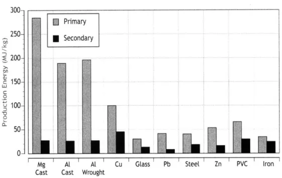
Figure 1-1 Production energy of various metals from primary or secondary sources

(K eoleian, Kar et al. 1997) ... . . ... ... ... ... 12 Figure 1-2 Recycling rate (old and new scrap consumed divided by total metal

consumption) and scrap recovery (scrap consumed divided by total scrap generated) for the past 50 years [Kelly et al., 2004] ... 13 Figure 1-3 Year-over-year change in US apparent consumption of aluminum, copper, iron, steel and nickel (Kelly, Buckingham et al. 2005) ... 15 Figure 2-1. Schematic representation of a two-stage recourse model. Specific decisions for the case analyzed in this paper are shown at bottom ... 23 Figure 3-1 Probability distribution function used for each finished good demand under th e B ase C ase... ... ... 3 1 Figure 3-2 Base Case Results (wrought scenario): Scrap purchasing for mean-based strategy (decision only on mean demand) and recourse-based strategy (decision based on probability distribution of demand) ... 34 Figure 3-3 Base Case Results (Cast Scenario): Scrap purchasing for mean-based strategy (decision only on mean demand) and recourse-based strategy (decision based on

probability distribution of demand) ... 35 Figure 3-4 costs breakdown on each demand scenario. ... ... 36 Figure 3-5 Impacts of magnitude of demand uncertainty on the hedging ratio. ... 38 Figure 3-6 Effects of scrap salvage value on scrap pre-purchase hedging strategy in w rought scenario ... ... ... 40 Figure 3-7 of scrap salvage value on scrap pre-purchase hedging strategy in cast scenario.

...4 0

Figure 3-8 Effects of scrap-to-primaries price ratio on scrap pre-purchase hedging

strategy in the wrought scenario ... ... 43 Figure 3-9 Effects of scrap-to-primaries price ratio on scrap pre-purchase hedging

strategy in cast scenario ... ... 43 Figure 3-10 Impacts of products' specification span on scrap usage, costs with both m od el. ... ... ... ... ... .... ... 4 6 Figure 3-11 comparisons among granularity of discrete probability states...47

Figure 3-12 Effects of granularity on the cost objective function ... 49

Figure 3-13 Effects of granularity on hedging ratio ... .... 49

Figure 4-1: Total Cost and probability density of each demand scenario for deterministic strategy of pre-purchasing D amount of scrap. Here we assume the mean demand is 20kT. ... ... ... ... 56

Figure 4-2: Total cost and possibility density of each demand scenario for recourse strategy of pre-purchasing H amount of scrap. Here we assume the mean demand is 20kT. ... 56

Figure 4-3: Comparison of the two strategies in terms of their total costs for each scenario. ... 57

Figure 4-4: Relationship between the hedging ratio and the scrap salvage value ... 59

Figure 4-5: Relationship between the scrap over primary ratio and hedging ratio. ... 59

1 Introduction

1.1 Metal Recycling

Recycling is crucial for the sustainability of non-renewable metal resources. Fortunately,

recycled scrap metals possess several intrinsic advantages over the primary materials for

which they substitute; these advantages create incentives for recycling.

First of all, most of the energy required for the production of primary aluminum is

embodied in the metal itself. Consequently, the energy needed to melt aluminum scrap is

only a fraction of that required for primary aluminum production. Recycling of aluminum

products needs only 5% of the energy needed for primary aluminum production (2008). It

is estimated that recycling of aluminum saves up to 6 kg of bauxite, 4 kg of chemical

products, and over 13 kWh of electricity, per kilogram of aluminum recycled (2005). The

energy consumption difference between the production of primary metals and the

recycling of secondary metals is shown in Table 1-1 and graphically in Figure 1-1. Given

the considerable positive environmental aspects of aluminum recycling, in addition to its

prevailing consumption globally, this thesis focuses on the recycling of this specific

metal. However, the approach and conclusions should be applicable to other metals, or

more broadly, natural resources.

In addition to the energy advantage, recycling of aluminum products emits only 5% of

the greenhouse gases emitted in primary aluminum production. Recycling of old scrap

now saves an estimated 84 million tons of greenhouse gas emissions per year. Since its

inception, the recycling of old scrap has already reduced CO2 emissions associated with

Table 1-1 Estimated Energy Savings Associated with Recycling Metals (Roberts 1983)

Metal Percent of Embodied Energy Saved

Aluminum 82

Copper 69

Zinc 38

Lead 97

Iron, Carbon Steel, Other Ferrous 39

Stainless Steel 20 00-3 21 2 1( 50

50-

0-Mg At At Cu Glass Pb Steel Zn I PVC Iron Cast Cast Wrought

Figure 1-1 Production energy of various metals from primary or secondary sources (Keoleian, Kar et al. 1997)

In the US, over the last four decades, secondary production has risen from 178,000 metric

tons per year to over 2,930,000 metric tons per year (Kelly et al., 2004), a growth rate

was more rapid than any other major metal over the same period. Recycling is a major

aspect of aluminum use, with more than a third of all the aluminum currently produced

globally originating from recycled metals. The aluminum recycling industry has

effectively tripled its output from 5 million tons in 1980 to over 16 million tons in 2006.

During the same time period primary metal use has grown from 15 to 30 million tons. 12

.N

i

L~~L4~FL

The proportion of recycled aluminum to the global demand for the metal has grown from

less than 20% in 1950 to approximately 33% in 2006. Of an estimated total of over 700

million tons of aluminum produced in the world since commercial manufacture began in

the 1880s, about three quarters of that total is still in productive use, at least in part thanks

to the recycling industry. The recycling rate and scrap recovery rate in the US are shown

in Figure 1-2. Despite the significant increase in the recycling rate, the aggregate

aluminum recycling rate still seldom exceeds 50%. The goal of this work is to identify

approaches that could increase the financial incentives to secondary aluminum consumers

to utilize more recycled aluminum.

6 0 %. . .. .· . . . .. ... ... .... 30% 20% :i -- Recycing Rate 10% Scrap Recovery

0 % ...

...

.

.

...

...

Figure 1-2 Recycling rate (old and new scrap consumed divided by total metal consumption) and scrap recovery (scrap consumed divided by total scrap generated) for the past 50 years

[Kelly et al., 2004].

Adding incentives to increase recycling is the same as reducing the disincentives to

secondary materials consumers to collect and process secondary material ([Goodman et al., 20051 and [Wernick and Themelis, 19981). A significant set of economic

disincentives emerges due to various types of operational uncertainty that confront

secondary processors ([Khoei et al., 20021, [Peterson, 19991 and [Rong and Lahdelma, 20061). For instance, relevant sources of operational uncertainty include facts that a supplier may deliver raw materials late or not at all; warehouse workers may go on strike;

items in the inventory may be of poor quality; demand for your product may go up or

down; the composition of the raw materials might vary, etc. These uncertainties have the

largest adverse effect on those furthest from the customer, e.g. materials producers, due

to the feedback mechanisms inherent in typical market-based supply-chains (Lee et al.,

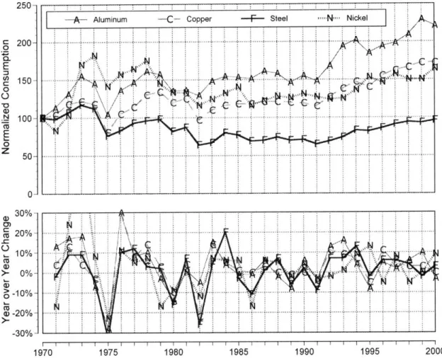
1997.) An appreciation of the specific uncertainties facing metal processors can be gained

by examining the historical volatility of aggregate US demand for a number of basic

metals. Figure 1-3 illustrates annual demand from 1970 to 2000. For all of the metals

plotted, there is significant variability in consumption from period to period with variance

ranging from 5% to 20%. (Kelly, Buckingham et al. 2005). Nevertheless, despite real

C 200-0 E O N 100 E Z 50- n-30%-o cr 3%

i ....

.

.

I... ...

Figure 1-3 Year-over-year change in US apparent consumption of aluminum, copper, iron, steel and nickel (Kelly, Buckingham et al. 2005).

1.2 Previous Work on Operational Uncertainty

A range of research activities have been motivated by the significant environmental and

economic benefits of secondary materials recycling. This research can be broadly

classified into two categories: technological evolution and new decision-making methods.

On the technological side, the focus has been on developing new equipment and

processing methods to improve the quality of scrap while minimizing its variability, such

as sorting technologies that are being developed to control variability in chemical

15

-A--- Aluminum -- -- Copper -F-- Steel N" Nickel "

..... ... . .. . . .I ... : i i A / X

.'..

....

...

...

·i·...i.

i.·j.·

···...

···

_911-F

···

11

·

--:-:~~--~-

·

I

compositions of scrap streams. (Maurice, Hawk et al. 2000; Gesing, Berry et al. 2002;

2003; 2003; Mesina, Jong et al. 2004; Reuter, Boin et al. 2004). For instance, Maurice et

al suggest a thermo-mechanical treatment to establish conditions that cause fragmentation

of cast material, while wrought material, having lost much less of its toughness, merely

deforms. The two types of product could then be separated by simple sizing methods

(Veit 2004).

Similarly, there are many research activities exploring improved decision-making

methods concerning accommodating various operational uncertainties. For example,

Gaustad et al explored the use of a chance-constrained optimization method to explicitly

consider the scrap's compositional uncertainty and showed that it is possible to increase

the use of recycled material without increasing the likelihood of batch errors compared to

a conventional deterministic method.

Other work has focused on decisions of individual processors. One approach considers

the questions of whether and to what extent specific technological or operational options

should be employed to reduce costs or increase profits. (Lund, Tchobanoglous et al. 1994;

Stuart and Lu 2000; Stuart and Qin 2000) Another approach considers the identity and

quantity of raw materials that should be purchased and allocated to production. (Shih and

Frey; Cosquer and Kirchain) Similarly, analytical models combined with simulations of

materials flows have been applied to guide the allocation decisions of materials across the

processors within an entire recycling system (van Schaik, Reuter et al. 2002; van Schaik

and Reuter 2004; 2004b). Nevertheless, all the work above modeled future demand

deterministically. This thesis will model and analyze the environmental and economic

impacts with the demand uncertainty treated stochastically.

There is other work that folds in demand uncertainties into decision-making, but this

concentrates mainly on reduction in total demand uncertainty and takes the residual

uncertainty as irreducible systematic risk. For example, Kunnumkal et al suggested an

operating service agreement between suppliers and customers that requires the supplier to

provide customers with incentives to minimize their demand uncertainty through

activities such as acquiring advance demand information, employing more sophisticated

forecasting techniques, or smoothing product consumption. The resulting reduction of the

demand uncertainty brings benefits to both parties. This thesis looks into a method to

gain such benefits under an operational environment with irreducible demand uncertainty.

The operations management literature has also examined the impact of uncertain demand

on a range of manufacturing decisions. A particularly relevant concept, "safety stock,"

was studied extensively in the field of inventory management and product designs as

early as the 1950s. "Safety stock" is a term used to describe a level of stock that is

maintained above the expected stock requirement to buffer against stock-outs. Safety

stock, or buffer stock, exists to counter uncertainties in supply and demand (Atkins 2005).

Safety stock is held when an organization cannot accurately predict demand and/or lead

time for a product. For example, if a manufacturing company were to find itself

continually running out of inventory, it would determine that there is a need to keep some

extra inventory on hand so that it could meet demand while the main inventory is

replenished. In other words, maintaining a stock of components greater than that dictated

by the expected demand (that is, a safety stock) can have production service and economic advantages.(Arrow, Harris et al. 1951; Dvoretzky, Kiefer et al. 1952; Clark and

shared by multiple products) allow service levels' to be maintained with reduced safety

stock. (Dogramaci 1979; Collier 1982; Baker, Magazine et al. 1986; Graves 1987) These

principles have been applied to nearly all forms of operations, manufacturing and service,

as well as supply chain management and product or system design.(Guide Jr and

Srivastava 2000) However, across all of the cases identified by the author, models and

insights have focused on products made of discrete components. Recently, this work has

been extended to include cases where some amount of component substitution is possible

(i.e., where more than one component can meet the production demands for a single

product or multiple products). (Bassok, Anupindi et al. 1999; Geunes 2003; Cai, Chen et

al. 2004; Gallego, Katircioglu et al. 2006) However, reported work is limited to cases

where the number of combinations of components that can produce the desired finished

good is finite. For materials production, there is an infinitely continuous number of

combinations of raw materials that can be used to make a finished good that still satisfies

specifications. Effectively, there is a substitute for nearly every raw material in nearly

every product with some combination of other raw materials. As a consequence, it is not

possible to directly apply the methods or insights developed to-date to materials

production decisions.

To examine the implications of demand uncertainty within materials production, this

thesis work develops a schematic analytical framework that explicitly comprehends the

1 Service level is measure of performance of an inventory system. It measures the probability that all customer orders arriving within a given time interval will be completely delivered from stock on hand, i.e. without delay, or measures the proportion of total demand within a reference period which is delivered without delay from stock on hand.

impact of demand uncertainty 2 in the context of materials production from primary and

secondary raw materials. The specific modeling method applied is a linear

recourse-based optimization model. The results of this model are contrasted against the results of

more traditional scrap management decision-making in which forecasts are formed using

a deterministic framework.

Methods that comprehend uncertainty - whether they be based on models, simulations,

analysis, or notional frameworks - are always more analytically demanding. However,

such methods have been shown in a range of contexts to enable more effective or

efficient use of resources - capital, natural and financial. (previously cited references on

manufacturing safety stocks as well as Shih and Frey 1995; Geldof 1997; AI-Futaisi and

Stedinger 1999; Gardner and Buzacott 1999; Ralls and Taylor 2000 and the balance of

papers within the special issue of Conservation Biology; Skantze and Ilic 2001; Peterson,

Cumming et al. 2003; de Neufville 2004) Through the use of the recourse-based model,

this thesis explores the extent to which and the contexts in which such benefits exist for

materials production.

In Chapter 2, the modeling framework will be built up, which will be used as a major tool

to conduct a general case study in Chapter 3 to show the benefits of the approach. In

order to better understand the benefits, an important feature on multiple products

portfolio is studied in Chapter 4 compared to single product portfolios. An analytical

2 Notably, _{the magnitude of product demand is only one form of uncertainty that confronts secondary} material producers. Others include quantity of available supplies, the composition of delivered raw materials, and the pricing of both raw materials and salable products. The method presented herein is readily extensible to address at least two of these - uncertainty in availability and prices. Considerations of raw material compositional uncertainty require other, non-linear modeling methods.

expression for the hedging ratio with a simplified case was derived and discussed in

2 Modeling Framework

This chapter is devoted to establishing a recourse-based model framework with the

explicit consideration of demand uncertainty that can identify driving forces for

improvement in scrap consumption by secondary metal producers.

Traditionally, metal producers, purchase scrap based on point forecasts of the demand for

future periods. In contrast, the model built up in this chapter will take into account the

uncertain demand. The detailed comparisons in the case study in the next chapter will

examine the benefits of such scrap purchasing strategy change. Case results will show

that alloy production planning solely based on expected demand leads to more costly

production and less scrap usage on average than planning derived from more explicit

treatment of uncertainty. The short but intuitive explanation is that the later approach

utilizes more information, i.e., demand variance, by pricing in the benefits/penalties

associated with all possible demand scenarios. The benefits will be further studied and

expressed analytically in chapter 4 in a rigorous form.

2.1 Overview of Recourse Modeling

The most widely applied and studied stochastic programming models are two-stage linear

programs. In such models, the decision maker is represented as taking some action in a

first stage, after which a random event occurs affecting the implications of the first-stage

decision. A recourse decision can then be made in the second stage that attempts to

compensate for negative effects that might have been experienced as a result of the

first-stage decision and the revealed future conditions. The output from such an optimization

defining which second-stage action should be taken in response to each random outcome

(Petruzzi and Dada 2001; Cattani, Ferrer et al. 2003). This methodology can be applied

towards a wide variety of problems including resource planning, financial planning, and

even communication network design (Martel and Price 1981; Growe, Romisch et al. 1995;

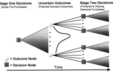
Kira, Kusy et al. 1997; Dupacova 2002). In a simple two-stage model as in our case, at

stage one a set of decision needs to be made to prepare for a given stochastic event. After

the event happens, i.e. the stochastic process ends up with a deterministic outcome, a

corrosponding set of stage-two decision will be made to accomodate it. In the context of

our case, at the stage-one time point, the producers have to pre-purchase an amount of

various scraps, before demand from downstream consumers is known. The scrap

materials pre-purchasing strategy here is the stage-one priori decision based on all

possible demands scenarios. When orders from aluminum alloy consumers arrive (i.e. the

previously uncertain demand data are revealed), a set of posteriori raw materials

(primaries and alloying element) purchasing plans need to be made accordingly. This

decision making scheme for a two-stage context is illustrated in Figure 2-1, in which

Stage One Decisions Uncertain Outcomes Stage Two Decisions

(Scrap Pre-Purchases) (Potential Demand Outcomes) (Primaries & Alloying

S= o

S=De

Figure 2-1. Schematic representation of a two-stage recourse model. Specific decisions for the case analyzed in this paper are shown at bottom.

The general objective function for a recourse problem consists of two parts shown as the

following.

f(C, D')+ g(C, p, D2

)

Eq 2-1

In Eq 2-1, the contribution from stage one to the objective function is given by the

function

f(.).

characterize quantitatively the state of the decision. The contribution from stage two to

the objective function is given by the function g(.). D2 is the vector of stage-two recourse

variables over all possible outcomes and p is the vector of the probabilities of those

outcomes. The overall cost impact of the recourse decisions to the overall objective are weighted by those probabilities. In other words, the objective is an expected objective

rather than a deterministic objective. C is the cost vector whose aggregate contribution to

the objective function is being maximized or minimized in an optimization problem. In addition, within the model, various constraints are imposed that must be satisfied for all

23

stage decisions. Such constraints allow the model to reflect more accurately case specific

conditions.

2.2 Recourse Model with Demand Uncertainty for Alloy Producers

A linear programming model is employed with a recourse framework for the cost of alloy production utilizing both scrap and primary raw materials. The mathematical definition of

the model is given in Eq 2-3 to Eq 2-8. The goal of this model is to minimize the overall

expected production costs of meeting various finished goods demand through an optimal

choice of raw material purchases and allocations. By accounting for the probabilities and

magnitude of demand variations, the model optimizes the cost of every possible demand

scenario weighted by the likelihood of those scenarios. The primary outcome from such a

model will define both a scrap pre-purchasing strategy as well as a set of production

plans (including primary and alloying element purchasing schedules) for each demand

scenario. Effectively, this provides an initial strategy and a dynamic plan for all known

events. The variables to solve for are D S, Disf and D2pf which will be defined

subsequently together with other notations.

Minimize:

Eq 2-2 C',D' + CPzDp - PSaIvC, P R

p,f,z s,z

subject to

Eq 2-3 D

R,

=

D

-

-

D;=

Eq 2-4 /

For each demand scenario z there are scrap supplies constraints as determined by the

amount of scrap pre-purchased,

ED' <D1

Eq 2-5 f

Eq 2-5 enforces the aforementioned condition that scrap materials must be ordered before

final production. As such, at production time, no more scrap can be used than was

ordered. Similarly, a production constraint exists for each scenario, quantifying how

much of what alloy must be produced:

ED' +

= B:

Eq 2-6 P

For each alloying element c, the composition of each alloy produced must meet

production specifications (Datta 2002):

D

DU•,. U< + E DaU, < BizUi

Eq 2-7 P

I D

SDTfL,

_z

₊

_{D L,}

_{2 B}

f

Lf,

Eq 2-8 P

All other variables are defined below:

R, = Residual amount of scrap s unused in scenario z

C, = unit cost of primary material p

D's = amount (kt) of pre-purchased scrap material s

P- = probability of occurrence for demand scenario z

Psaiv = salvage value out of the original value of the residual scrap materials

D2pf- = amount of primary material p to be acquired on demand for the production of

finished good

funder

As = amount of scrap material s available for pre-purchasing

Dlsf = amount of scrap material s used in making finished goodf under demand scenario

z

Bft amount of finished goodf produced under demand scenario z

Mf: = amount of finished goodf demanded under demand scenario z

UsC = max. amount (wt. %) of element c in scrap material s

Lsc = min. amount of element c in scrap material s

Upc = max. amount of element c in primary material p

LpC = min. amount of element c in primary material p

Ufc = max. amount of element c in finished good f

Notably, in the model formulation shown above, the total cost includes those incurred by

scrap and primary materials, and excludes the salvage value percentage Psaiv of those

residual scrap materials if any. Residual scrap occurs when the demand was insufficient

to consume all of the scrap which was pre-purchased in stage one. It is critical to note

that residual scrap that was pre-purchased has embodied value. It can be resold or used

for future production. In deterministic analyses, no unused scrap will ever be purchased

since any unneeded scrap will simply drive up costs, making its existence irrational. In

the stochastic environment, some extra scrap might be pre-purchased that will be useful

on average but will lead to unused scrap in certain scenarios. To get a reasonable estimate,

an assumption has been made that the salvage value will be at a discount to the cost of

acquiring that scrap material. The discount is assumed to be 5% in most of the following

case study scenarios if not specified to be different one. One interpretation of this

discount is time value of money. Another is the cost of storage of this unused material.

In future work the impact of this parameter should be quantified separately and more

precisely. To be complete, it should also be noted that the salvage value is not always at

a discount to the original cost of acquisition. In a rising scrap price environment or tight

supply market (Gesing 2002), the rise in price can more than offset factors such as time

value of money or cost of storage. The objective function also factors in the probabilistic

nature of the demand outcomes. This modifies the effects of expected primary usage as

3 Case Study

3.1 Case Description

With the modeling framework established in the last chapter, the usefulness of the above

formulation can be more clearly shown through its application in a case study.

Specifically, the cases examine the purchasing and production decisions of a secondary

remelter. The question being asked is what raw materials should be purchased now and at

production time and how should these be mixed to produce finished goods demanded

(ordered) by the customer. More generally, this case is used to explore the ability of this

modeling framework to provide novel insights for the management of secondary

resources.

For the purposes of the case analysis while keeping the generality, we simultaneously

consider two production portfolios. One consists of four of the most popular cast Al

alloys (319, 356, 380 and 390); the other includes four popular wrought Al alloys (3105,

5052, 6061 and 6111). These alloys were chosen because of their prevalence within

overall industry production and should be illustrative of results for similar alloys. In

addition to a full complement of primary and alloying elements, the modeled producer

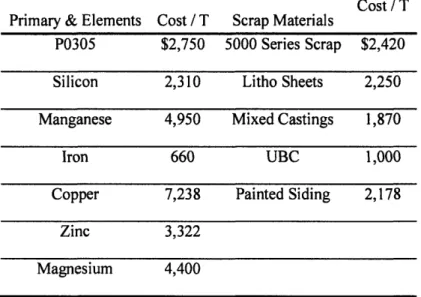
has available five post consumer scraps from which to choose. Prices and compositions

used within the model for both input materials and the finished alloy products are

summarized in Table 3.1, II and III, respectively. Notably, the case examines production

for two portfolios of four finished goods (cf. Table 3.3) from twelve raw materials (cf.

Table 3.1) - five scrap and seven primary materials. Average prices on primaries as well

The scrap prices were quoted from globlescrap.com. The scraps types and compositional

information are taken from studies by Gorban reflecting scrap materials that might be

expected to derive from the automobile. (Gorban, Ng et al. 1994) Finished goods

compositional specifications are based on international industry specifications. (Datta

2002) Base case salvage value of any residual scrap, S, is assumed to by 95% of original

value unless specified.

Table 3.1. Prices of raw materials used for case analysis Primary & Elements

P0305 Silicon Manganese Iron Copper Zinc Magnesium

Table 3.2. Compositions of scrap "Year 2000" vehicle) Cost / T $2,750 2,310 4,950 660 7,238 Scrap Materials 5000 Series Scrap Litho Sheets Mixed Castings UBC Painted Siding Cost / T $2,420 2,250 1,870 1,000 2,178 3,322 4,400

materials used for case analysis (from (Gorban, Ng et al.) Average Compositions (wt. %) Si Mg Fe Cu Mn Zn Raw Materials 5000 Series Scrap 0.23 _{1.88 0.38 0.08 0.45} 0.19 Litho Sheets 0.08 0.60 0.00 0.64 0.13 0.64 Mixed Castings _{10.13 0.23 0.83 2.63 0.38} 0.90 UBC 0.04 0.23 0.98 0.38 0.15 0.83 Painted Siding 0.38 0.75 0.45 0.60 0.60 0.38

I

I

r

I

Table 3.3. Finished goods chemical specifications used for case analysis (Datta) Finished Goods

Cast Fir

Zn

Si Mg Fe Cu Mn

nished Goods Portfolio

Min 0.75 319 6.25 0.08 0.75 3.75 0.38 Max 0.25 5.75 0.03 0.25 3.25 0.13 Max 0.04 7.25 0.41 0.22 0.08 0.04 356 _Min 0.01 6.75 0.34 0.16 0.03 0.01 Max 2.25 9.00 0.15 1.50 3.75 0.38 380 _Min 0.75 8.00 0.05 0.50 3.25 0.13 Max 0.08 17.50 1.09 0.98 4.75 0.08 390 _{Min 0.03} 16.50 0.66 0.33 4.25 0.03 Wrought Finished Goods Portfolio

Max 0.19 0.70 2.00 0.53 0.34 0.11 3105 Min 0.06 0.50 1.20 0.18 0.21 0.04 Max 0.15 0.34 2.65 0.34 0.08 0.08 5052 Min 0.05 0.11 2.35 0.11 0.03 0.03 Max 0.19 0.70 1.10 0.70 0.34 0.11 3061 Min 0.06 0.50 0.90 0.00 0.21 0.04 Max O. 11 1.00 0.88 0.30 0.80 0.38 6111 Min 0.04 0.80 0.63 0.10 0.60 0.23

In order to ensure that results are not biased towards any particular product type, all four

finished goods were modeled using the same average demand and demand distribution, as shown in Figure 3-1. Specifically, the demand for all four alloys in both portfolios was

modeled with a mean of 20kt each and a coefficient of variation3 _{of 11%. Although}

finished good demand may be more accurately represented by a continuous function, the

probability distribution was discretized for these analyses to leverage the computational

efficiency and power of linear optimization methods. This approach also matches well

with common approaches of and information available to production planners.

(Choobineh and Mohebbi 2004) As shown in Figure 3-1, for the purposes of this case

analysis, each finished good has five possible demand outcomes, symmetric around the

mean. Considering all four alloys together, these conditions define 625 possible demand

scenarios (i.e., 54 from five possible outcomes for each of the four finished products). The

model formulation can be executed as presented with finer probability resolution, but at

the expense of greater computational intensity, and more importantly, the difference in

the total expected cost introduced by granularity is marginal, as we shall see in the later

discussion. ... .. .. .. ... ... .. ... .. ... .. .. .. .... ... .... ... ... .. . W0, 5. 0%. .....

....

...

Figure 3-1 Probability distribution function used for each finished good demand under the Base Case.

3 Defined as a/i where a _{is the standard deviation and ýi is the mean.}

31 ... ... ... ... ... ... . ............ ... ... ... ... ... ... .......

Amp

For the Base Case presented subsequently, all raw materials were assumed to be

unlimited in availability. The effects of this assumption were explored and are described

later in this paper. The model framework presented herein can be used for cases of

non-uniform demand and constrained scrap supply with no structural modification.

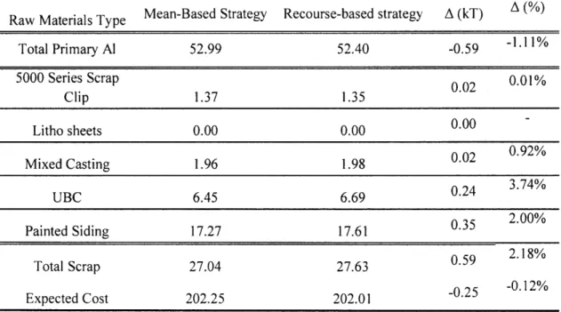
3.2 Base Case Results: Comparing Conventional and Recourse-Based Approaches The scrap purchasing strategy generated by the Recourse-Based and Mean-Based model

as well as summary costs and primary usage are presented in Table 3.4 and for the

wrought production portfolio and Table 3.5, for the cast production portfolio. Even with

only an 11% coefficient of variation (i.e., the Base Case assumptions), sizeable increases

in the modeled purchasing of certain scrap types can be seen with the Recourse-based

strategy in both portfolios. In aggregate, that strategy drives modeled scrap purchasing up

by around 2%. Notably, the Recourse-based strategy does not drive up the consumption

of scrap uniformly across the various scrap materials. As shown in column 5 of Table 3.4

and Table 3.5, the additional scrap purchases range from 0% for Litho Sheet to 3.74% for

UBC in the wrought portfolio production and range from 0% for 5000 series scrap to 2.68%

for mixed castings in the cast portfolio. Finally, for this Base Case comparison, the

expected cost savings derived from the Recourse-based strategy was $0.25M and $0.44M

for each scenario compared with the more traditional Mean-based approach. The

difference in purchased quantities that emerges between the two modeling strategies will

be referred to through the balance of the thesis as a hedge. Just like more conventional

financial hedging, this scrap hedge provides insurance against the need for purchasing

expensive primary materials. Specifically, the scrap hedge emerges because the

outweighed by the economic benefits of having the scrap when demand is high. As such,

the existence of the hedging purchases is driven by the potential for high product demand.

From an environmental perspective, it is notable that the Recourse-based method does

not only drive additional scrap purchases, but the existence of these purchases enables

additional expected scrap consumption. This increased scrap consumption does not

compromise the ability to use scrap in low demand scenarios. In fact, for some cases the

existence of pre-purchased scrap should drive occasional hyper-optimal scrap usage.

Table 3.4. Mean-based production portfolio

and Recourse-based approaches comparison on wrought alloys

Raw Materials Type Total Primary Al 5000 Series Scrap Clip Litho sheets Mixed Casting UBC Painted Siding Total Scrap Expected Cost Mean-Based Strategy 52.99 1.37 0.00 1.96 6.45 17.27 27.04 202.25 Recourse-based strategy 52.40 1.35 0.00 1.98 6.69 17.61 27.63 202.01 A (kT) -0.59 0.02 0.00 0.02 0.24 0.35 0.59 -0.25

A (%)

I

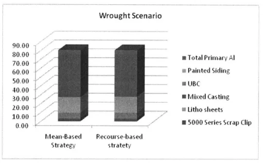
Wrought Scenario a Total Primary Al a Painted Siding a UBC * Mixed Casting 0 Litho sheets

i 5000 Series Scrap Clip Recourse-based

stratety

Figure 3-2 Base Case Results (wrought scenario): Scrap purchasing for mean-based strategy (decision only on mean demand) and recourse-based strategy (decision based on probability distribution of demand)

Table 3.5. Mean-based production portfolio

and Recourse-based approaches comparison with cast alloys

Raw Materials Type Mean-Based Strategy Recourse-based strategy A (kT) A (%)

Total Primary Al 43.27 42.39 -0.88 -2.04% 5000 Series Scrap Clip 0.00 0.00 Litho sheets 11.45 11.71 0.25 2.20% Mixed Casting 19.42 19.94 0.52 2.68% UBC 0.00 0.00 0.00 Painted Siding 5.88 5.98 0.11 1.85% Total Scrap 36.75 37.63 0.88 2.40% Expected Cost 197.35 196.92 -0.44 -0.22% 90,00 80.00 70.00 60.00 50.00 40.00 30.00 20.00 10.00 0.00 Mean-Based Strategy I *·.'' _,-." r :·: .·" g 'I .···'· i j.; ... .. .. .. .. -... ..-.... T...- ...-.. ... ..

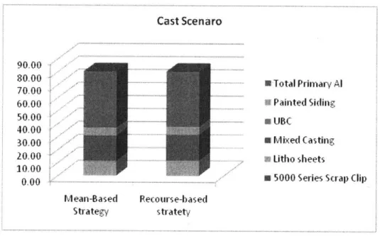
Cast Scenaro I Total Primary Al V Painted Siding as UBC a Mixed Casting ... Litho sheets .... :/II r.nf'n ( • 1 • .•+r.. ' l. 0.00 ... . Mean-Based Strategy

M )'I1 -)V - W-5 UPI aI., J V

Recourse-b ased stratet.

Figure 3-3 Base Case Results (Cast Scenario): Scrap purchasing for mean-based strategy (decision only on mean demand) and recourse-based strategy (decision based on probability distribution of demand).

3.3 _{Cost Breakdown in each demand scenario}

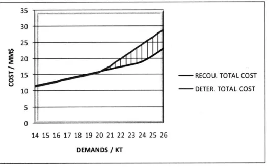
In terms of the total expected cost, the recourse-based model provides cost saving, as well as more scrap utilization. However, this aggregate behavior does not bear out for each scenario as shown in Figure 3-4. The cross-over point is when demand slightly exceeds its expected value, i.e. 20kT. Before the mean demand, the deterministic model incurs less cost. The reason for this behavior is that the demand is so low that the pre-purchased scrap for either strategy will not be fully consumed. Thus, the lesser pre-purchase of scrap materials associated with the deterministic scenario leads to lower inventory levels with less storage cost. However, when the demand soars beyond the expected demand, the excess storage of cheaper scrap will benefit the recourse strategy. Notably, the magnitude of cost difference on the two sides of the cross-over point is significantly different. This is also the key why the recourse model generates purchasing and

90.00

...

...

production plans that outperform the deterministic model. The intuitive explanation is in

high demand scenario, the availability of excess scrap saves the cost of approximately the

Figure 3-4 costs breakdown on each demand scenario.

difference between the primary materials and the scrap materials. However, the excess

amount of scrap inventory will incur a cost equivalent to 5% of the unused scraps value

while in a lower demand scenario. This is can be understood as cost of carry, which sets

an upper bound limit for pre-purchasing more scrap than enough for the expected demand.

In summary, the excess amount of scrap pre-purchase in recourse-based model is actually

a hedge against more costly and riskier high demand scenario. The cost of the hedge is 5%

of any scraps left after meeting all the demands. The term "hedging" will be mentioned

frequently in the thesis hereafter with this meaning.

30

--- RECOU. TOTAL COST - DETER. TOTAL COST

3.4 Exploring the Impact of Model Assumptions

The degree of hedging derived from a Recourse-based modeling approach will

undoubtedly depend on the operating conditions of a specific remelter. The most

pertinent assumptions include the underlying demand uncertainty, raw materials pricing

conditions and scrap availability constraints. Given that operating conditions can be

expected to evolve between the initial stage of planning and the final stage of materials

production, it is important to have a sense of how the hedge should evolve in response to

such changes. The following explores the impact of these factors.

3.4.1 Impact of Magnitude of Demand Uncertainty on Hedging

In the Base Case, at approximately 10% demand uncertainty, the benefits derived from

the Recourse-based strategy were $0.25M and $0.44M respectively in cost savings,

0.59kt and 0.88kt increase in average scrap usage for both portfolios. These benefits are

expected to rise with increasing product demand uncertainty.

In fact, for modifications on the Base Case, as the level of demand uncertainty increased

from 10% to 30%, the increase in scrap consumption went from 0.59kt and 0.88kt to

1.77kt and 2.64kt, the associated cost savings increased from $0.25M and $0.44M to

$0.77M and $1.32M for the wrought and cast portfolio respectively. Recall that the hedging purchases emerge from a favorable balance between the costs of carrying

additional scrap when demand is low and the savings realized when demand is high. As

long as this favorable balance exists, as uncertainty increases the hedge basket grows to

satisfy possible high demand scenarios. As with the Base Case results, increased hedging purchases drive higher expected scrap use and higher economic benefit in comparison to

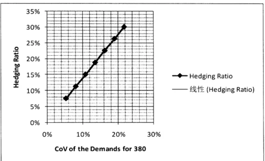
that associated with the traditional deterministic modeling approach. The explicit test on

the relationship between the demand uncertainty and the hedging ratio is run with the

model. Notably, Figure 3-5 shows a linear correlation between both quantities. The

underlying theoretical exploration will be demonstrated in

Figure 3-5 Impacts of magnitude of demand uncertainty on the hedging ratio.

3.4.2 Impact of Salvage Value on Hedging

In the results presented thus far, an assumption has been made that unused scrap

materials have salvage value equal to 95% of their original costs. Deviation from this

assumption would be expected to have an impact upon modeled optimum scrap

pre-purchasing strategy. Figure 3-6 and Figure 3-7 illustrate the sensitivity of the magnitude

of the hedge to scrap salvage value for both wrought portfolio and cast portfolio. The Okt

line is a reference for the mean-based strategy. Results are shown for two values of

demand variation. The most notable feature of this figure is that the hedge is not always positive. Ultimately, two factors affect the desirability of additional scrap purchase. One

35%

30%

is the potential cost savings that can be derived from having cheaper scrap materials to

use when needed (price differential advantage). The other is the net cost of carrying that

scrap material (carrying cost) until it leaves inventory, especially for low demand (i.e.,

low scrap usage) cases. The carrying cost can be defined as the acquisition price of the

raw material less the salvage value of the raw material. If the salvage value of the scrap

is too low, the carrying cost will more than offset the price differential advantage such

that purchasing and storing less scrap will be advantageous - leading to a negative hedge.

The difference between the two driving forces for hedging, namely cost savings from the

price differential less the carrying cost will be termed the option value of scrap. The

hedge will be positive (negative) when the option value is positive (negative).

The hedge was positive under the Base Case because the price differential advantage

outweighs the carrying cost of those scraps, giving a positive option value4. As Figure 3-6

and Figure 3-7 illustrate, below approximately 60% salvage value, the hedge no longer

provides value and shrinks to zero. In fact, below this point, it is better to have less scrap

on hand than implied by the mean-based strategy. At around 60% salvage value, the cost

of carrying an extra unit of scrap is perfectly balanced by the price differential advantage

from having that extra unit.

4 Option value of scrap: The difference between the two driving forces for hedging, namely cost

savings from the price differential less the carrying. The hedge will be positive (negative) when the option value is positive (negative).

Wrought Scenario 4 3

-1

--

-

--

-2

Figure 3-6 Effects of scrap salvage value on scrap pre-purchase hedging strategy in wrought scenario. Cast Scenario 8 I ... ... ... ... .... ... ... ... .. . . ... .. ... -4-10% CoV -a-20% CoV 0% Salvage Percentage

Figure 3-7 of scrap salvage value on scrap pre-purchase hedging strategy in cast scenario.

From Figure 3-6 and Figure 3-7 it is apparent that the hedge as a function of increasing salvage value is convex. This can be understood by considering separately the effects of

the two option-value driving forces. As the salvage value drops (to the left in the graph), 40

there is a tendency to purchase less scrap because the carrying cost is increasing. But

while lower salvage value implies higher carrying cost, having less scrap material also

denies the material system of the price differential advantage stemming from the price

difference between scraps and primaries. This price differential advantage is independent

of the salvage value. These two effects oppose each other, resulting in a slow rate of

decrease in the hedging amount in low salvage value environment. On the other hand,

when the salvage value is high the price differential advantage remains while the cost of

carry is also reduced. This double positive in higher salvage value environment is the

momentum behind the convexity observed in Figure 3-6 and Figure 3-7.

The option value is also intimately tied to the magnitude of the underlying demand

uncertainty. Larger uncertainties imply higher option value and result in greater driving

forces for hedging. When the price differential advantage more than offsets the carrying

cost, greater demand uncertainty will translate this effect into more positive hedging.

Similarly, when the carrying cost dominates, greater demand uncertainty will exacerbate

the situation by pushing for less scrap purchasing (i.e., more negative hedging). Hence, it

is observed in Figure 3-6 and Figure 3-7 that with greater demand uncertainty, the curve

rotates inward (counter-clockwise).

3.4.3 Impact of Secondary/Primary Price Gap on Hedging

Variations in the price differential advantage also affect the option value of scrap, which

in turn affect the degree of hedging. Since each raw material has its own price, the price

gap depends on the definition of the secondary price and primary price. According to Table 3.1, the variance of raw materials' prices is insignificant comparing to prices

themselves. Therefore, for simplicity, secondary material prices are defined as the 41

average price of all scraps used during the production, while primary materials' price are

the cost of producing if no scraps were available, i.e. only pure aluminum and alloying

elements can be used. Figure 3-8 and Figure 3-9 study the effect on the Base Case hedge

of the gap between secondary and primary prices for both portfolios, represented here as

the ratio between those two quantities. At the critical point of roughly 100% secondary to

primary price, the Recourse-based model suggests no additional scrap purchase above

that suggested by the mean-based method. At higher secondary prices, the hedge

becomes negative.

As discussed previously, the option value of scrap increases with demand uncertainty.

This effect is manifested in Figure 3-8 and Figure 3-9 in that with greater uncertainty,

the net offsetting effects of the carrying cost and the price differential advantage is

magnified, leading to a clockwise rotation of the curve. Specifically, above a price ratio

of around 100%, the carrying cost dominates over the price differential advantage.

Therefore, in this region the hedge is negative and the effect is magnified when the

underlying demand uncertainty increases. Once again, at a price ratio of about 100%, the

forces of the price-differential advantage and the carrying costs are just balanced. As

such, regardless of what the underlying demand uncertainty is, the hedge, which can be

Wrought Scenario

7

5

-13 4 50% 70% ..... 110%

in the wrought scenario. in the wrought scenario.

Cast Scenario 12 10 4

0 -

--- ---

-

--

-

1&

6

Scrap Price / Primary Price

-u-210% COV

--aE- 2

O'Xý

0

VV

pre-purchase hedging strategy

-- 10% CoV -- 20% CoV

Figure 3-9 Effects of scrap-to-primaries price ratio on scrap pre-purchase hedging strategy in cast scenario.

As secondary and primary prices converge, the price differential advantage goes to zero.

Therefore, the downward trend with increasing scrap-to-primaries price ratio is no _ _1~ --·1111111 ;.~...~~..._...._...

surprise. The observed concavity is due to different system constraints on either end of

the price ratio spectrum. When the price ratio is close to one, there is no barrier against

the drop in the hedge amount except of course that the overall scrap purchase cannot go

below zero. As long as this point is not reached, the hedge will continue to dive. When

the price ratio is low, the price differential advantage is large. However, even if the ratio

goes to zero (scrap is free), the increase in the hedging amount will not accelerate. The

mismatch in the compositions between scrap materials and the products sets a scrap

consumption limit. Only so much scrap can be used by the production before it becomes

physically impossible to meet compositional constraints.

Interestingly, Figure 3-8 and Figure 3-9 also shows that while the overall trend is for the

hedge to decline with higher scrap prices, there are regions over which the response is

relatively insensitive. Notably, such effects were not apparent in Figure 3-6 and Figure

3-7. The relative insensitivity versus that of the hedging amount towards the salvage

value is apparent from the formulation of the objective function. In Figure 3-6 and Figure

3-7, as the salvage ratio varies only the carrying cost of scrap is changing; the price

differential advantage is constant. Therefore, the sensitivity of the hedge towards the

salvage ratio is entirely driven by the change in the carry cost. However, in Figure 3-8

and Figure 3-9 as the price ratio varies both the carrying cost and the price differential

advantage are changing. Nevertheless, the carrying cost is changing very slowly. When

the price differential between scrap and primaries rises by 5%, the carrying cost only

goes up by 5% x (1 - 95%) = 0.15%. The choppiness in Figure 3-8 and Figure 3-9 is

The convexity and concavity observed in Figure 3-6, Figure 3-7 and Figure 3-8, Figure

3-9 gives the planner a sense of how frequently the hedge should be adjusted by buying

and selling scraps. The absolute distance between these curves and the zero-hedge

reference line can be taken as a measure of potential for cost savings. For instance, when

the salvage ratio is low, a small change in the ratio does not change this potential

significantly. However, in high salvage ratio regions, the hedge is much more sensitive

and as such should be monitored and adjusted more frequently. Similarly when the price

ratio between scraps and primaries is large, the hedge should be adjusted more frequently

than when the price ratio is low.

3.4.4 Variation in the width of the specification

In reality, scrap composition has significant uncertainty. In current practice, this variation

is accommodating by producing to a narrower finished products specification than is

actually required by the customer. Specification width is defined as the maximum

boundary minus the minimum boundary allowed. Figure 3-10 explores its impact on

expected costs of both models and scrap usage increase as well. The x-axis is percentage

of the specification span compared to the original one. First of all, the specification span

does not affect the validity of the advantage of recourse model strategy, i.e., both cost

saving and scrap usage increase exist. Secondly, scrap usage increase in percentage and

cost savings stays relatively similar with the change in span despite a significant change

in the total expected costs. The reason for the inflection point for the expected costs is

that a more expansive alloying element becomes binding when the width of the

specification shrinks below 60% for wrought case. The cast case will have the same behavior.

lu 1 25 S 20 15 t 10 5 S)U.UUVo 45.00% 40.00% - 35.00% b 30.00% r-25.00% _t X "20.00% -15.00% L -10.00% 5.00% U.UU70 0% 20% 40% 60% 80% 100% 120%

Width of Finished Goods Specification

--- Expected Cost Recouse Model -4 Expected Cost Determ. Model

-- Scrap Usage Increase

Figure 3-10 Impacts of products' specification span on scrap usage, costs with both model.

3.4.5 Impact of the discrete probability distribution of demands

As part of the modeling framework setting, the probability distribution of demands which

is continuous in reality has been discretized. The natural questions risen would be if this

approach will qualitatively or quantitatively change the hedging behavior, how many

discrete states would be appropriate if hedging behavior is still valid for cost saving and

scrap usage enhancement. Clearly, there is a big difference in terms of possible states and

their possibilities of happening if continuous distribution were discretized into 5, 25 or

256 discrete states as shown in Figure 3-11. The more states the probability distribution is

split into, the closer it is to representing the underlying distribution. However, with n

products and m uncertain demand scenarios, the total possible outcomes for the problem

at hand are mn, which scales rapidly with the totally number of discrete states. Is the 5

discrete states used in the case study so far are sufficient to capture the real hedging

behaviors in practice?