Publisher’s version / Version de l'éditeur:
Stochastic Environmental Research and Risk Assessment, 22, pp. 1-15, 2008-01-01
READ THESE TERMS AND CONDITIONS CAREFULLY BEFORE USING THIS WEBSITE.
https://nrc-publications.canada.ca/eng/copyright
Vous avez des questions? Nous pouvons vous aider. Pour communiquer directement avec un auteur, consultez la première page de la revue dans laquelle son article a été publié afin de trouver ses coordonnées. Si vous n’arrivez pas à les repérer, communiquez avec nous à [email protected].
Questions? Contact the NRC Publications Archive team at
[email protected]. If you wish to email the authors directly, please see the first page of the publication for their contact information.
NRC Publications Archive
Archives des publications du CNRC
This publication could be one of several versions: author’s original, accepted manuscript or the publisher’s version. / La version de cette publication peut être l’une des suivantes : la version prépublication de l’auteur, la version acceptée du manuscrit ou la version de l’éditeur.
For the publisher’s version, please access the DOI link below./ Pour consulter la version de l’éditeur, utilisez le lien DOI ci-dessous.
https://doi.org/10.1007/s00477-006-0090-1
Access and use of this website and the material on it are subject to the Terms and Conditions set forth at Probabilistic risk analysis using ordered weighted averaging (OWA) operators
Tesfamariam, S.; Sadiq, R.
https://publications-cnrc.canada.ca/fra/droits
L’accès à ce site Web et l’utilisation de son contenu sont assujettis aux conditions présentées dans le site
LISEZ CES CONDITIONS ATTENTIVEMENT AVANT D’UTILISER CE SITE WEB.
NRC Publications Record / Notice d'Archives des publications de CNRC: https://nrc-publications.canada.ca/eng/view/object/?id=9dbc920f-4a20-4079-8946-1fea91938912 https://publications-cnrc.canada.ca/fra/voir/objet/?id=9dbc920f-4a20-4079-8946-1fea91938912
http://irc.nrc-cnrc.gc.ca
P r o b a b i l i s t i c r i s k a n a l y s i s u s i n g o r d e r e d
w e i g h t e d a v e r a g i n g ( O W A ) o p e r a t o r s
N R C C - 4 9 2 2 7
T e s f a m a r i a m , S . ; S a d i q , R .
A version of this document is published in / Une version de ce document se trouve dans: Stochastic Environmental Research and Risk Assessment, v. 22, no. 1, Jan. 2008, pp. 1-15 doi: 10.1007/ s00477- 006- 0090- 1
The material in this document is covered by the provisions of the Copyright Act, by Canadian laws, policies, regulations and international agreements. Such provisions serve to identify the information source and, in specific instances, to prohibit reproduction of materials without written permission. For more information visit http://laws.justice.gc.ca/en/showtdm/cs/C-42
Les renseignements dans ce document sont protégés par la Loi sur le droit d'auteur, par les lois, les politiques et les règlements du Canada et des accords internationaux. Ces dispositions permettent d'identifier la source de l'information et, dans certains cas, d'interdire la copie de documents sans permission écrite. Pour obtenir de plus amples renseignements : http://lois.justice.gc.ca/fr/showtdm/cs/C-42
Probabilistic risk analysis using ordered weighted averaging (OWA)
operators
Solomon Tesfamariam
Institute for Research in Construction, National Research Council Canada, Ottawa, Ontario Canada K1A 0R6
Tel: (613)-993-2448; Fax: (613)-993-1866 E-mail: [email protected]
and
Rehan Sadiq1
Institute for Research in Construction, National Research Council Canada, Ottawa, Ontario Canada K1A 0R6
Tel: (613)-993-6282; Fax: (613)-993-1866 E-mail: [email protected]
1
Abstract
The concepts of system load and capacity are pivotal in risk analysis. The complexity in risk analysis increases when the input parameters are either stochastic (aleatory uncertainty) and/or missing (epistemic uncertainty). The aleatory and epistemic uncertainties related to input parameters are handled through simulation-based parametric and non-parametric probabilistic techniques. The complexities increase further when the empirical relationships are not strong enough to derive physical-based models. In this paper, ordered weighted averaging operators (OWA) are proposed to estimate the system load. The risk of failure is estimated by assuming normally distributed reliability index. The proposed methodology for risk analysis is illustrated using an example of nine-input parameters. Sensitivity analyses identified that the risk of failure is dominated by the attitude of a decision-maker to generate OWA weights, missing input parameters and system capacity.
Keywords: system load and capacity, reliability, ordered weighted averaging (OWA), uncertainty, ignorance, probabilistic risk analysis.
LIST OF NOTATION
δ Degree of a polynomial function
α Degree of orness
) (r
Q Linguistic quantifier as a fuzzy subset to generate OWA weights )
(r
Q∗ Linguistic quantifiers “for all” to generate OWA weights )
(r
Q∗ Linguistic quantifiers “there exists” to generate OWA weights
max Maximum (parameter for Uniform distribution)
μ Mean (normal distribution) Z
μ Mean of the performance function
C
μ Mean of the system capacity
L
μ Mean of the system load
s Measure of scatter (lognormal distribution)
o
X Median (lognormal distribution)
min Minimum (parameter for Uniform distribution)
Φ Cumulative probability function for a standard normal distribution
T n w w w , , , ) (
w = 1 2 L OWA weight vectors
j
w OWA weights
Z Performance function
f
P Probability of system failure
∗
k rapping
rations in MCS Realizations or iterations in Bootst
k Realizations or ite
β Reliability index
θ Scale parameter (Weibull distribution)
w
m Shape parameter (Weibull distribution) σ Standard deviation (normal distribution)
Z
σ Standard deviation of the performance function
C
σ Standard deviation of the system capacity
L
σ Standard deviation of the system load ity th * * * ,..., , k k k x x
x s for input parameters generated randomly for k
n x
,..., ters generated randomly for MCS
i)
C System capac
L System load
j
b The j largest element in the vector (X1, X2,…, Xn)
Vector of value 2 1 n Bootstrapping k 2 k 1,x
x Vector of values for input parame F(X Cumulative distribution function
m Number of historical data points S tstrapping A eraging P2 distributions function 1, X2,…, Xn Input parameters
MC Monte Carlo simulation
n Number of input parameters
N Number of realizations in MCS
N* Number of realizations in Boo
OW Ordered weighted av
p Probability of event
P1 and Parameters of the probability
PDF Probability density
1. Introduction
Rowe (1977) defines risk as the potential for unwanted negative consequences of an event or an activity, whereas Lowrance (1976) defines it as a measure of probability and severity of negative adverse effects. Risk analysis may be defined as the estimation of the frequency and physical consequences of undesirable events, which can produce harm (Ricci et al., 1981). The concepts of demand or load ( ) and capacity (C) of a system are pivotal to risk analysis. The input parameters to compute load and capacity are generally prone to uncertainties that propagate through the
analysis, which ultimately influence the risk estimates. The uncertainties related to input parameters can be categorized as: aleatory (variability) uncertainty as a result of natural heterogeneity or
stochasticity, which cannot be reduced; and epistemic uncertainty, is due to partial ignorance or subjectivity, which can be reduced with the availability of more information. Traditionally in risk analysis, aleatory and epistemic uncertainties can be referred to as risk and uncertainty, respectively (Paté-Cornell, 1996). Knight (1921) made a distinction between risk and uncertainty; risk is where mathematical probabilities can be assigned either through a priori knowledge or from the statistics of past experience, whereas uncertainty is referred to randomness, which cannot be explained. The epistemic uncertainty considered in this paper is related to the missing information of input parameters, and lack of physical based model in congruence with Knight’s interpretation of uncertainty. Consequently, for missing input data, the minimum (worst) and maximum (best) possible values (an interval) are used without making any uniform distribution assumption and consequently interval-valued risks are produced.
L
The term ‘system’ is context dependent, which can be referred to civil engineering structures like bridges, water distribution systems and treatment plants, or to environmental systems like a river, stream or ambient air quality. In the context of environmental risk assessment, L is the exposure of contaminants to receptors through air, water or food. In case of building structures, L can be the external loading, e.g. wind, snow, and/or earthquakes. System capacity C on the other hand is the maximum allowable load or minimum acceptable strength the system is capable of bearing. The C can be evaluated through physical models or acceptable threshold limit are specified from standards, guidelines or self-imposed limits. Generally, these threshold limits are context or scenario dependent e.g., intended use of the water (e.g. for bathing, drinking) requires its own specific capacity Cor regulatory guideline. Similarly, different threshold limits are established for building structures based on their intended use (e.g., nuclear facility, residential buildings).
The system load (or capacity)2 can be estimated using a physical-based model with known (or assumed) mathematical relationships. However, for complex systems, these relationships are not readily available due to lack of understanding or information (Klir, 1985; Ayyub and Chao, 1997). The main thrust of this paper is to evaluate the risk of failure of a system for which physical-based (or empirical) models are not available. A soft computing based method is proposed to ‘aggregate’ the non-commensurate input parameters in a meaningful way without explicitly knowing the model, i.e., under ignorance. This requires that the input parameters to be in a commensurable unit before
2
In the subsequent sections, the system capacity is assumed a priori known information, either through regulatory guidelines or expert provided data. However, the proposed methods to compute system load is equally applicable.
aggregation. This concept is similar to a scoring method. In this case, fuzzy operators are used to aggregate data in the absence of a physical-based model.
Aggregation of fuzzy sets requires operations by which several fuzzy numbers are combined in a desirable way to produce a single fuzzy number (Klir and Yuan, 1995). The literature reflects numerous ways and operators to aggregate data, e.g., conjunctive (and-type) operators like
minimum, product (also known as t-norms) and disjunctive operators (or-type) like maximum,
summation (also known as s-norms). The aggregation process in a probabilistic framework uses
product for ‘and’, and summation (for mutually exclusive events) for ‘or’. Other common operators
for aggregation are known as compromising operators, which include arithmetic, geometric and harmonic means.
The aggregation operators have their own share of shortcomings, especially the recognition of two potential pitfalls, namely exaggeration and eclipsing, is important. Exaggeration occurs when all input parameters are of relatively low importance, yet the aggregate score comes out unacceptably high. Eclipsing is the opposite phenomenon, where one or more of the input parameters are of relatively high importance, yet the aggregated score comes out as unacceptably low. The type of an aggregation operator typically affects these phenomena. Therefore, the challenge is to determine the best aggregation operator, which will simultaneously reduce both exaggeration and eclipsing (Ott, 1978).
In this paper, ordered weighted averaging (OWA) operators (Yager, 1988) are proposed to estimate the system load. The OWA operators are commonly used for decision-making under partial or complete ignorance (Yager, 2004). The concept of OWA is explored in various disciplines of engineering and artificial intelligence and many nuances and extensions have been proposed. The motive behind selecting the OWA operator for aggregation of input parameters is their capability to encompass a range of operators from minimum to maximum including various averaging
(compromising) operators like arithmetic mean. The OWA operator provides a flexibility to incorporate decision maker’s attitude or tolerance towards risk, which can also be related to the criticality of the particular system under investigation. The OWA operation involves three steps: (1) reordering of the input parameters; (2) determining the weights associated with the OWA operators; and (3) aggregation process.
To explain the concept of the proposed approach, this paper is structured based on an illustrative example of nine input parameters. The remainder of the paper is outlined as follows: Section 2 expounds the proposed methodology to perform risk analysis. It includes description of the use of OWA operators for aggregation, parametric and nonparametric techniques to perform probabilistic analysis, and finally discussion on risk analysis. Section 3 illustrates how to handle missing
information or data in risk analysis. Section 4 describes the results of sensitivity analysis using various forms of OWA operators. Section 5 provides a discussion and a summary of the paper.
2. Proposed methodology
Complex decision models often involve uncertain input parameters, which can be determined with varying degrees of accuracy. Different classical (probabilistic) and non-classical methods (including possibility theory, fuzzy sets, fuzzy measures, random sets) are used to represent different types of uncertainties. In this paper, stochastic input parameters are handled in a probabilistic framework using parametric and nonparametric techniques like Monte Carlo simulations and Bootstrapping, respectively. Parametric techniques require that input parameters be defined based on known or
assumed probability distributions. Defining probabilistic distribution a priori is a daunting task. However, where possible, a probabilistic distribution may be fitted to the historical data (frequentist approach) or may be defined subjectively based on expert judgment (Bayesian approach). In case of nonparametric techniques, defining a probability distribution is not a requirement; rather random samples are drawn from the historical data set.
After identifying and deciding on the simulation technique, the input parameters are aggregated using predefined OWA operators for each iteration or realization. The results of this aggregation provide an empirical distribution function (EDF) for the system load. Finally, for a given system capacity, the risk is estimated. A schematic of the proposed methodology is shown as a flow chart in Fig. 2.The proposed methodology has three distinct tasks – data processing (Section 2.2), data aggregation using OWA to estimate system load (Section 2.1), and risk analysis using the concepts of load and capacity to estimate the risk of failure (Section 2.3). As mentioned before, capacity is assumed to be provided by the expert who understands the system or it could be a regulatory specification. However for any complex system, the capacity can be estimated using the same procedure as proposed for the load. Further it is assumed that the system load and capacity are not correlated.
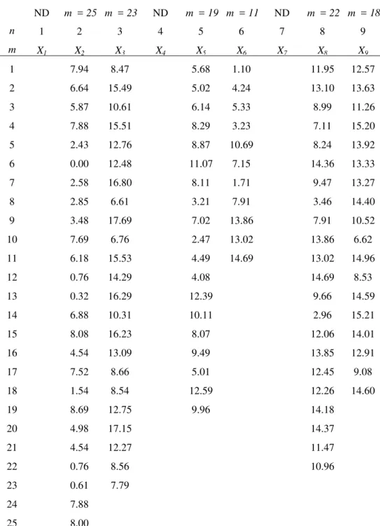
The proposed methodology is expounded using a 9-input parameters example (X1, X2,…, X9; n = 9)
given in Table 1. These 9-input parameters, for example, can be viewed as water quality indicators or parameters used in estimating building structure’s vulnerability against earthquake. It is assumed that all input parameters have commensurate units and do not require transformation before
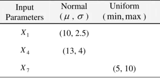
aggregation. Six out of the nine input parameters have varying number of historical data points (m) (Table 1). The remaining three-input parameters (X1, X4 and X7), have no historical data.
Consequently, ‘expert’ provided probability distribution functions are defined (Table 2).
2.1. Data aggregation
2.1.1. OWA operator: basic concepts
Most multi-criteria decision analysis problems require neither strict “anding” (like minimum) of the
t-norms nor strict “oring” of the s-norms (like maximum). To generalize this idea, Yager (1988)
introduced a new family of aggregation technique called the ordered weighted average (OWA) operators, which is a general mean type aggregator. The OWA operator provides a flexibility to utilize the whole range of “and” to “or” associated with the attitude of a decision maker in the aggregation process.
An OWA operator of dimension n is a mapping , which has an associated weighting vector . The requirements to be satisfied are
R Rn → n T n w w w , , , ) ( w= 1 2 L wj∈[0,1] and .
Hence, for given input parameters, the input vector (X
∑nj=1wj =1
n 1, X2,…, Xn) is aggregated using OWA
operators as follows:
∑
= = = n 1 j j j n 2 1,X , ,X ) w b X ( OWA L L (1) where bj is the j thlargest element in the vector (X1, X2,…, Xn) and . Therefore, the
OWA weight is not associated with any particular value X
n b b
b1 ≥ 2 ≥...≥
j
ordinal position of . The linear form of OWA equation aggregates a vector of input parameters (X
j b
1, X2,…, Xn) and provides a nonlinear solution (Yager and Filev, 1999).
The range of OWA between two extremes minimum and maximum can be expressed through the degree of orness(α), which is defined by Yager (1988) as follows:
(
)
∑
= − − = α n i i n i w n 1 ) ( 1 1 , and α∈[0,1] (2) The orness characterizes the degree to which the aggregation is like an or operation. For α = 0 refers to a case that OWA vector w becomes (0, 0,…, 1), i.e., an element with the minimum value in the multiple criteria vector (X1, X2,…, X9) gets the ‘full’ weight, which implies that the OWAbecomes a minimum operator. Similarly when α = 1, refers to a scenario that OWA vector w becomes (1, 0,…, 0), i.e., an element with a maximum value in the input parameters vector (X1,
X2,…, X9) is assigned ‘full’ weight, which implies that the OWA becomes maximum operator.
2.1.2. Determination of OWA weights
A class of functions to generate OWA weights, called regularly increasing monotone (RIM) quantifier was first proposed by Yager (1988). The RIM functions are bounded by two linguistic quantifiers “there exists” (or) and “for all”, (and). Thus, for any RIM quantifier , the limit holds true (Yager and Filev, 1994). The OWA weights can be
generated for a given RIM quantifier as follows ) (r Q∗ Q∗(r) Q(r) ) ( ) ( ) (r Q r Q r Q∗ ≤ ≤ ∗ ) (r Q ⎟ ⎠ ⎞ ⎜ ⎝ ⎛ − − ⎟ ⎠ ⎞ ⎜ ⎝ ⎛ = n i Q n i Q wi 1 i=1,2,...,n (3)
Yager (1988, 1996) defined a parameterized class of fuzzy subsets, which provides families of RIM quantifiers that change continuously between Q∗(r) and Q∗(r) by:
δ r ) r ( Q = r≥0 (4) (a) For δ =1; Q(r) = r the unitor quantifier (arithmetic average, i.e., = 0.5) α (b) Forδ →∞; Q∗(r), the universal quantifier (and-like, i.e., α = 0)
(c) Forδ →0; , the existential quantifier (or-like, i.e., Q∗(r) α = 1) Therefore Equation (3) can be generalized as
δ δ ⎟ ⎠ ⎞ ⎜ ⎝ ⎛ − − ⎟ ⎠ ⎞ ⎜ ⎝ ⎛ = n 1 i n i wi , i=1,2,...,n (5)
where δ is a degree of a polynomial function. For δ = 1, the RIM function becomes a uniform distribution, i.e., the weight distribution becomes similar to an arithmetic mean, i.e., wi = 1/n. For δ > 1, the RIM function leans towards right, i.e., “and-type” operators manifesting negatively skewed OWA weight distributions. Similarly, for δ < 1, the RIM function leans towards left (it becomes RDM, i.e., regularly decreasing monotone), i.e., “or-type” operators manifesting positively skewed OWA weight distributions.
A simple example is provided here to illustrate the OWA weight generation and aggregation process to estimate the load of the system. This example involves 9-input parameters (X1, X2,…, X9) with
commensurable values. It is also assumed that δ = 1/3. A three-step OWA operation is described as follows:
Step 1) Reordering of the input arguments X:
X = (X1, X2,…, X9) = (0.125, 0.423, 0.622, 0.233, 0.866, 0.251, 0.396, 0.168, 0.269)
After reordering (write in descending order)
(b1, b2,…, b9) = (0.866, 0.622, 0.423, 0.396, 0.269, 0.251, 0.233, 0.168, 0.125)
Step 2) Determining the weights associated with the OWA operators: Using δ = 1/3 and n = 9 in Eq. (5)
) w , , w , w ( 1 2 L n = (0.48, 0.12, 0.09, 0.07, 0.06, 0.05, 0.05, 0.04, 0.04) Step 3) Aggregating (system load) using Eq. (1):
L = 0.48 × 0.866 + 0.12 × 0.622 +…+ 0.04 × 0.125 = 0.61.
As mentioned before, the meaning of the system load L is context dependent.
2.2. Data Processing
All input parameters are assumed to contain only aleatory uncertainty to simplify the analysis. For input parameters X1, X4 and X7, the historical data are not available, but initially we assume that
reliable information on the type of distribution of data is provided (Table 2). Given the input parameters, data processing entails utilization of two stochastic techniques (parametric and nonparametric analyses). The following subsections will highlight both types of analyses.
2.2.1 Parametric analysis
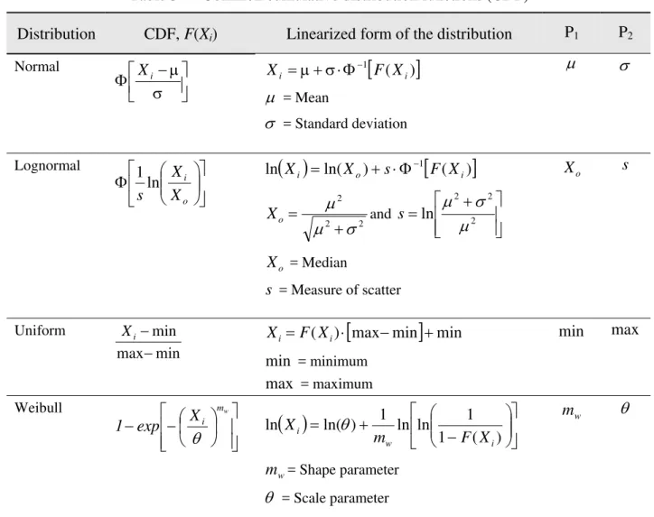
Parametric analysis requires defining the probability density functions (PDFs) for each input parameter. Monte Carlo simulations (MCS) and its derivatives are the most common simulation-based methods that fall in this category. As described earlier, historical data or expert knowledge are used to define the PDFs for input parameters. Commonly used PDFs, like normal, lognormal,
uniform and Weibull are selected in this example as candidate distributions for simplicity. Though proposed method is equally applicable to any type of PDF. Each of the selected PDFs can be
described using two parameters. The cumulative distribution function (CDF), and parameters of each distribution are provided in Table 3.
Continuing with the aforementioned example, statistical distributions are fitted to six input parameters (Table 1), , for which historical data are available. Four candidate distributions as mentioned earlier are fitted to the data of each input parameter, and the corresponding statistical parameters (P1, P2) are estimated.
9 8 6 5 3 2,X ,X ,X ,X ,X X
Fig. 3 shows the graphical representation of a fit of 4 candidate distributions to the input parameter . The criterion used for the goodness of
fit is the coefficient of determination (R
2 X 2
). The parameters of the fitted distributions are provided in Table 4. For example, the uniform distribution is the best-fitted model to the historical data of the input parameter X2. Table 4 also shows the best-fitted distribution for each input parameter in a shaded box. For input parameters X3,X5,X8, the normal distribution is found to be the best fitted
distribution, whereas Weibull distribution is the best fitted distribution for input parameters and . 6 X 9 X
Once the probability distributions of the input parameters are decided, Monte Carlo simulations (MCS) are performed and aggregation for each realization ( ) is done using OWA operator to determine the system load. The number of realizations (N) is chosen so that any increase in this number will not significantly change the statistical properties of the system load. The following steps are followed to determine the system load using MCS:
k
• From a predefined or best-fitted PDFs for each input parameter (X1, X2,…, Xn), draw a
random sample →k x1k,x2k,...,xnk,
• Repeat the sampling process for N realizations,
• Define the power of RIM quantifier (δ) associated with decision maker’s attitude (α), and
compute OWA weights,
• For each realization k, aggregate using the OWA to estimate the system load (Eq. 1),
= OWA( ),
L x1k,x2k,...,xnk
• Arrange the estimated system loads in an ascending order and assign the plotting positions to each iteration using mean rank formula, k/(N + 1), and
L
• Plot the empirical distribution function (EDF) and determine the mean and standard deviation of the EDF.
The EDF’s shape and magnitude of the system load generated through MCS depend on the decision maker’s attitude (α). Fig. 4 shows the EDFs generated from MCS at δ = 3, 1, 1/3, with
corresponding orness of α = 0.33, 0.5, 0.67, respectively. Fig. 4 shows that with an increase in , the EDF shifts towards the maximum values. To simplify the risk analysis, it is further assumed that the EDFs of the system load are normally distributed with estimated mean
orness
L
μ and standard deviation σ . Therefore, for δ = 3, 1 and 1/3, the system load distribution (L N μ ,L σ ) are L
(2.38, 0.54), (6.79, 0.90), and (11.46, 1.59), respectively.
N N N
2.2.2 Nonparametric analysis
Bootstrapping is a computationally intensive nonparametric simulation technique used for making inferences from historical data. Bootstrapping differs from the traditional parametric approach (like MCS) as it draws large numbers samples with replacement from the original data sets without making strong distribution assumptions (Efron and Tibshirani, 1986; 1993). Efron pioneered Bootstrap simulations in 1979 for estimating confidence intervals. The main advantage of
Bootstrapping is that it can provide estimates in the situations where mathematical solutions are not possible (Efron and Tibshirani, 1993).
Bootstrapping uses analogy between the sample and the population from which the sample is drawn. The central idea is that it may be better to draw conclusions about the characteristics of a population strictly from the sample at hand, rather than making ‘unrealistic’ assumptions about the population.
Bootstrapping involves re-sampling the data with replacement many times in order to estimate the statistics of interest. However, in this paper, instead of estimating a certain statistical parameter, the resample data points are directly used in the OWA operator. Bootstrapping is performed by
randomly sampling from the historical data of size m for a given input parameter Xi. The implementation of the generic Bootstrapping procedure is as follows:
• For each input value (where historical data are provided in Table 1) draw a random sample with replacement, (in our case for those input parameters for which historical data are not available MCS iterations are used),
∗
k x1k*,x2k*,...,xnk*
• Repeat the resampling process with replacements for N*
realizations,
• Define the decision maker’s attitude (α) through selecting power of RIM quantifier (δ) and
compute the corresponding OWA weights,
• For each realization , aggregate using the OWA operator, L = OWA(k∗ * *),
2 * 1 , ,..., k n k k x x x
• Arrange the estimated loads in an ascending order and find the plotting positions using mean rank formula, k
L
*
/(N* + 1), and
• Plot the empirical distribution function (EDF) and determine the mean and standard deviation of the EDF.
Resulting EDFs from the Bootstrapping using three levels of decision maker’s attitude, δ = 3, 1, 1/3 (corresponding α are 0.33, 0.5, 0.67, respectively) are shown in Fig. 5. Similar to the MCS, Fig. 5 shows that with an increase of orness, the results becomes closer to the maximum, and this
manifests in a right shift of the EDF. However, comparing the difference between the two extreme values α = 0.67 and 0.33 used in this analysis, the Bootstrapping captures less variability as compared to MCS. This can be explained in the light that no assumptions were made for the type of the distributions, consequently MCS may over or under estimate the variability depending on the type of distribution selected. The EDF of the system load are assumed normally distributed
(
orness
N μ ,L σ ). Thus, from Fig. 5, for δ = 3, 1, 1/3, the resulting system load distributions are L
(6.00, 1.13), (9.01, 0.93), and (11.85, 1.03), respectively.
N N N
2.3. Risk analysis
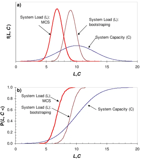
Risk analysis is a method of accounting for the risks in a particular engineering system resulting from various sources of uncertainty. When the load exceeds its capacity (Fig. 1), failure of the system is imminent; therefore the risk3 is computed as the probability of load exceeding capacity,
p(C<L). To compute the probability or risk of failurePf , a performance function Z can be
mathematically expressed as: ); 0 ( < = p Z Pf where Z = C - L (6) 3
Various methods are available to perform probabilistic risk analysis, such as analytical or numerical integration, simulation, response surface method, or first- and second-order reliability methods. Obtaining solution for Eq. (6) is complex, as it requires double integration over and C domains (Melchers, 1987). The most common approach is safety margin (SM) or performance function approach, which is the difference between capacity and value calculated for design loading (Eq. 6). This method involves linearizing the limit state function at the design point and then determining the value of the reliability index
L
β, which satisfies the limit state function. Theβis a measure of safety or functionality of the system. The normal distribution is used widely to relate safety factors to reliability when small variations in dimensional tolerances are expected. Similarly when the uncertainty about the load or capacity or both is large, the lognormal distribution is useful (Lewis, 1987). For simplicity, in the subsequent discussion and computation of risk of failure, it is assumed that both load and capacity have normal distribution. For normally distributed safety margin, the mean μ and standard deviation Z σ of Z are computed as follows: Z
L C Z μ μ μ = − 2 L 2 C Z σ σ σ = + (7)
and the reliability index is β
2 L 2 C L C Z Z σ σ μ μ σ μ β + − = = (8)
Consequently, the risk of failure Pf is ) ( 1 ) (−β = −Φ β Φ = f P (9)
where Φ is the cumulative distribution function (cdf) for a standard normal distribution. Similar relationships can be derived for lognormal distribution of system load and capacity. In Eqs. (7-9), it is assumed that the system load and capacity are uncorrelated and completely random. However, if the correlation between them is established through data or known a priori, the above equations can be modified accordingly (Cornell et al. 2002). In case of positively correlated load and capacity, the estimated risk of failure will be lower than the risk estimated from Eq. (9), i.e., a case of
uncorrelated system load and capacity. In contrary, if the relationship is negatively correlated, the estimated risk of failure will be higher than the uncorrelated estimates of risk.
Assume the system capacity C is normally distributed with mean μC = 10 and standard deviation C
σ = 3, i.e., N (10, 3). This example is illustrated using system load EDF for polynomial function
δ = 1. The PDF of the system load for MCS and bootstrapping and corresponding system capacity are shown in Fig. 6a. The system load EDFs using MCS and Bootstrapping, and corresponding system capacity EDF are plotted in Fig. 6b. The load EDFs are normally distributed for both MCS:
(6.79, 0.90) and bootstrapping: (9.01, 0.93). Thus, for estimated system load using MCS (6.79, 0.90) and given system capacity
N N
Consequently, the corresponding risk of failure is = 0.15. Thus, it can be interpreted that the risk of failure is = 0.15 and reliability of the system is 0.85. Similarly, for the bootstrapping, the reliability index β = 0.32 and corresponding risk of failure is = 0.38. Based on these two risk estimates, it can be interpreted that bootstrapping is more conservative, since it has higher risk of failure. f P f P f P
3. Dealing with missing information
The proposed methodology so far was made with an assumption that information for every input parameter is available either through historical data or through expert judgment. In cases where information for certain input parameters are missing, however, decisions are made under partial ignorance (Yager, 2004). Thus, for the missing input parameters, the decision maker can use two extreme possible values, which leads to interval-valued EDFs of system load. This concept is explained by assuming that the expert provided information in Table 2 is not available. Rather, only minimum and maximum values of the missing information are provided. To expound on the
proposed methods, three scenarios are considered, 1-miss, 2-miss and 3-miss. For the 1-miss scenario, the information for is missing (i.e., , and are known); for the 2-miss scenario, the information for and are missing (i.e., is known); and for the 3-miss scenario, information for all three input parameters, , , and , are missing. The minimum and maximum values considered for , , and are (2.5, 17.5), (1, 25) and (5, 10), respectively.
1 X X4 X7 1 X X4 X7 1 X X4 X7 1 X X4 X7
The system capacity C is again assumed to be normally distributed with a mean μC = 10 and
standard deviation σC = 3, i.e., N (10, 3). Further, the baseline results is the 0-miss analysis with δ
= 1. The δ = 1 assumption represents result of an arithmetic average, which represents a
compromising attitude. The risk analysis discussed in the previous section was performed for the three scenarios. The computation procedure for missing information scenarios remains the same as outlined earlier in Section 2. However, in case of missing information of a given input parameter, the analysis and simulation is repeated twice. The general steps to compute interval-based using MCS is outlined for 1-miss scenario as follows:
f P
• Assign value of X1 = 2.5
• From a predefined or best-fitted PDFs for each input parameter (X2,…, X9), draw a random
sample →k x2k,...,x9k,
• Repeat the sampling process for N realizations, • Assign the power of RIM quantifier δ = 1
• For each realization k, aggregate using the OWA to estimate the system load (Eq. 1),
= OWA( ,
• Arrange the estimated system loads in an ascending order and assign the plotting positions to each iteration using mean rank formula, k/(N + 1),
L
• Plot the empirical distribution function (EDF) (Fig. 7) and determine the mean and standard deviation of the EDF, N (5.97, 0.89),
• Calculate the risk of failure using Eqs. (7-9), Pf = 0.10, and
• Repeat the same process with X1 = 17.5, and finally obtain N(7.62, 0.83) and Pf = 0.22. The system load EDFs computed using MCS are shown in Fig. 7. Fig. 7a shows the EDF for the 0-miss analysis, with the corresponding risk of failure isPf= [0.15, 0.15] (from Section 2). Fig. 7b illustrates the interval EDF of 1-miss scenario and the corresponding risk of failure is = [0.10, 0.22]. Similarly,
f P
Fig. 7c and 7d show results of 2-miss and 3-miss scenarios, and the corresponding risk of failures are Pf = [0.10, 0.55] and Pf = [0.06, 0.52], respectively.
For the 1-miss scenario, the change in small. However, the upper bound of the = 0.22 shows more variation from the baseline (0.22-0.15 = 0.07) than the lower bound (0.15-0.10 = 0.05). This is due to the nonlinear nature of the OWA aggregation and the order of ’s minimum and maximum values with respect to the other input parameters. In light of this, it can be interpreted that the order of ’s minimum value has relatively less dominance than the order of ’s maximum value. Both f P Pf f P 1 X 1 X X1
Fig. 7c and Fig. 7d show an increase in the (epistemic) uncertainty band that highlights the significance and dominance of the missing information. It is interesting to note that for 2-miss scenario, the minimum = 0.10 is not different from the 1-miss scenario. This shows that the minimum value selected for (1) is not showing any significance in the final system load computation. However, the reverse is true, where the sensitivity of the maximum value is
reflected in the final . On the other hand, the 3-miss scenarios, showed a decrease in the minimum and higher sensitivity in the maximum value of .
f P 4 X 4 X f P f P Pf
Similar results are observed for the bootstrap simulations (Fig. 8). The baseline 0-miss results are provided in Fig. 8a, where the risk of failure is Pf = [0.38, 0.38]. The Pf for the 1-miss (Fig. 8b), 2-miss (Fig. 8c) and 3-2-miss (Fig. 8d) scenarios are [0.36, 0.57], [0.18, 0.69], and [0.18, 0.75],
respectively. For all analyses, the band of uncertainty for Bootstrapping is wider than the MCS. The above description provides a rigorous approach of dealing with the missing data without making assumptions about probability distribution. The interval-valued EDFs for load provide a realistic view to the decision maker on what can be the possible range of risk estimates.
4. Sensitivity analysis
Sensitivity analysis enables the identification of critical input data/parameters (Cullen and Frey 1999) that have a significant impact on the risk of failure. Central to the proposed model is the use of OWA operator for data aggregation. Initial sensitivity analysis using the degree of polynomial δ = 3, 1, 1/3 showed that there is a marked difference in the final EDF of the system load and the
corresponding estimates of risk of failure.
Now the sensitivity analysis is extended to δ = 1/9, 1/5, 1/3, 1, 3, 5, 9 for both MCS and
bootstrapping. First, the analysis is carried out for a 0-miss scenario. Once the EDF of the system load is established, the statistical values like average, 10th and 90th percentile are reported. The results of the MCS and bootstrapping are shown in Fig. 9 and Fig. 10, respectively. Both figures show that with an increase in δ (i.e., decrease in ), the mean value of system load L decreases. Moreover, results of the MCS (
orness
Fig. 9) show that an increase in δ causes a decrease in variability (can be interpreted as a difference between 10th and 90th percentile values). However, the bootstrapping results (Fig. 10), contrary to the MCS results, show less reduction in variability with an increase in
δ. This is attributed to the difference in the minimum values sampled in the MCS and bootstrapping.
In MCS, the random sample can be picked beyond the historical data minimum (or maximum) value as shown in Table 1. On the contrary, for the bootstrapping, the sample minimum and maximum is fixed to the values given in Table 1. Consequently, with δ = 1/9, the minimum value gets the highest weight, and minimum values selected in the MCS are dominant.
Summary of the sensitivity analyses results for both MCS and bootstrapping are provided in Table 5. Table 5 also shows the difference in upper and lower risk estimates using MCS
( )
ΔMCS andbootstrapping
( )
ΔBS . As discussed before, with an increase in number of missing input parameters at given δ , the ΔMCSand ΔBS values increase. For the 0-, 1- and 2-miss scenarios, maximumdifferences are obtained at δ =1/3. However, for the 3-miss scenario, the maximum difference is obtained at δ =1. At δ = 9, i.e. orness α ≈ 0, Table 5 shows that the risk of failure is 0. ≈ So far, the sensitivity analysis is carried out for system capacity with μ =10 and C = 3, with a
coefficient of variation COV =
C
σ
C
σ /μC=3/10 = 0.30. The sensitivity analysis is repeated by varying
the system capacity mean value (μC) and COV (Fig. 11). The MCS simulation is carried out for two
degree of orness, α = 0.67 (δ = 1/3) and α = 0.33 (δ= 3), and the risk of failure is shown contour plots in
f P
Fig. 11a and Fig. 11b, respectively. The risk of failure contour plot is illustrated for = 7.5 and COV=0.60. Hence, the corresponding values for
C
μ Pf α = 0.67 and α = 0.33 are 0.80,
and 0.13, respectively. As expected (Fig. 11a) a decrease in the system capacity mean μC, causes an
increase in Pf . For example, for μC=15 and COV = 0, the risk of failurePf ≈ 0, and for μC=5 and COV = 0, Pf ≈1. Fig. 11a shows that at μC= 5, the interval estimate of the risk of failure is big
= [0.1, 0.95]. However, with for
f
P μC= 15, the interval estimate of the risk of failure is reduced to = [0.43, 0.88]. It can be seen that for a given system load, by decreasing
f
P μC and fixing σ , the C
risk of failure increases. This has direct implication in the regulatory threshold for capacity. The risk contour plot coupled with
f P
Fig. 11b shows that the risk of failure is not sensitive to the variation of μC, due to the fact that the
estimated system’s load for α = 0.33 is small. However, the risk of failure showed relatively higher sensitivity with variation in COV, Pf ≈ [0.02, 0.22].
5. Discussion and Summary
One of the basic premise in the use of OWA operator is that the input parameters are in
commensurable units. For simplicity, in this paper commensurate values of input parameters were assumed. However, this is not always be the case. Therefore non-commensurate input parameters are transformed into commensurate units. Fig. 12 shows four commonly used transformation functions that can be used for this purpose. These functions include monotonically increasing function (MIF), monotonically decreasing function (MDF), and non-monotonic function that could be convex (CxF) or concave (CvF) function. Selection of these functions depends on the type of input parameters (attributes). A detailed discussion on this subject is beyond the scope of this paper. However, once non-commensurate input parameters are transformed into commensurate values, the methodology explained in this paper is valid.
The proposed methodology can be opted for systems for which physical-based models are not available. The methodology is flexible enough to handle the case of scant and missing data. If all stochastic input parameters are available, the corresponding output is a point estimate of risk. However, in case of missing information, the risk estimates are interval-valued. Interval-valued risk of failure is important as it reflects the state of knowledge about the system and guides decision maker to make informed decisions under partial ignorance. This concept is similar to belief and plausibility used in Dempster-Shafer theory. Generally, beliefs manifest themselves at two levels - the credal level (from credibility) where belief is entertained, and the pignistic level where beliefs are used to make decisions. The term “pignistic” was proposed by Smets (2000) and originates from the word pignus, meaning ‘bet’ in Latin. Pignistic probability is used for decision-making and uses Principle of Insufficient Reason to derive a point estimate. Therefore, interval-valued risk can be transformed into pignistic probability for decision-making under partial ignorance. See Sadiq et al. (2006) for details.
A summary and specific conclusions of the proposed methodology are as follows:
• The proposed OWA operators can be used in lieu of complex modelling and for decision-making under partial ignorance where physical-based models are not available;
• Aleatory uncertainty is handled through stochastic analyses using parametric (Monte Carlo simulations) and nonparametric (bootstrapping) techniques;
• Missing information (epistemic uncertainty) is handled using interval-valued stochastic analyses;
• The decision-maker’s attitude (degree of orness) is the dominant parameter in the final risk estimates, which is followed by the number of missing input parameters. With increase in number of missing input parameters, the epistemic uncertainty is reflected in a large interval-valued risk of failure Pf ; and
References
Ayyub, B.M. and Chao, R.-J. 1997. Uncertainty types and modeling methods. Uncertainty Modeling and Analysis in Civil Engineering, edited by B.M. Ayyub – CRC Press, Boston, pp.1-28.
Cornell, C.A., Jalayer, F., Hamburger, R.O. and Foutch, D.A. 2002. Probabilistic Basis for 2000 SAC Federal Emergency Management Agency Steel Moment Frame Guidelines. ASCE Journal of Structural Engineering, 128: 526-533.
Cullen, A.C., and Frey, H.C. 1999. Probabilistic Techniques in Exposure Assessment: a Handbook-for Dealing with Variability and Uncertainty in Models and Inputs. Plenum Press, New York, pp. 352.
Effron, B., and Tibshirani, R. (1986). Bootstrap methods for standard errors, confidence intervals, and other measures of statistical accuracy. Statis. Sci., 1: 54–77.
Effron, B., and Tibshirani, R. (1993). An Introduction to the Bootstrap. Chapman and Hall, Inc., New York.
Hohenbichler, M. and Rackwitz, R. (1981). Non-normal dependent vectors in structural safety. Journal of the Engineering Mechanics Division, ASCE, 107(6): 1227-1238.
Klir, G.J. (1985). Architecture of Systems Problem Solving, Plenum Press, New York.
Klir, G.J. and Yuan, B. (1995). Fuzzy Sets and Fuzzy Logic: Theory and Applications. Upper Saddle River, NJ: Prentice Hall International.
Knight, F. (1921). Risk, Uncertainty, and Profit. Boston, Haughton Mifflin.
Lewis, E.E. (1987). Introduction to Reliability Engineering. John Wiley & Sons, New York. Lowrance, W. W. (1976). Of Acceptable Risk. Los Altos, CA: William Kaufmann.
Melchers, R.E. (1987). Structural reliability: analysis and prediction. Chichester, England: Ellis Horwood.
Ott, W.R. (1978). Environmental Indices: Theory and Practice. Ann Arbor Science Publishers, Michigan, US.
Paté-Cornell, M.E. (1996). Uncertainties in risk analysis: six levels of treatment. Reliability Engineering and System Safety, 54: 95-111.
Ricci, P.F., Sagen, L.A., and Whipple, C.G. (1981). Technological Risk Assessment Series E: Applied Series No.81.
Rowe, N. (1977). Risk: An Anatomy of Risk. John Wiley and Sons, NY.
Sadiq, R., Kleiner, Y. and Rajani, B. (2006). Estimating risk of contaminant intrusion in distribution networks using Dempster-Shafer theory of evidence, Civil Engineering and Environmental Systems, 23(3): 129-141.
Smets, Ph. (2000). Data Fusion in the transferable Belief Model, Proceedings of 3rd International Conference on Information Fusion, Fusion 2000, pp. PS21-PS33, Paris, France, July 10-13 Yager R.R. (1996). Quantifier guided aggregation using OWA operators. International Journal of
Intelligent Systems, 11: 49–73.
Yager, R.R, and Filev, D.P. (1999). Induced ordered weighted averaging operators. IEEE Transactions System Man and Cybernetics, 29: 141–150.
Yager, R.R. (1988). On ordered weighted averaging aggregation in multicriteria decision making. IEEE Transactions on Systems, Man and Cybernetics. 18: 183-190.
Yager, R.R. (2004). Uncertainty modeling and decision support. Reliability Engineering and System Safety, 85: 341-354.
Yager, R.R. and Filev, D.P. (1994). Parameterized "andlike" and "orlike" OWA operators. International Journal of General Systems, 22: 297-316.
Table 1 Data for input parameters used in the example ND m = 25 m = 23 ND m = 19 m = 11 ND m = 22 m = 18 n 1 2 3 4 5 6 7 8 9 m X1 X2 X3 X4 X5 X6 X7 X8 X9 1 7.94 8.47 5.68 1.10 11.95 12.57 2 6.64 15.49 5.02 4.24 13.10 13.63 3 5.87 10.61 6.14 5.33 8.99 11.26 4 7.88 15.51 8.29 3.23 7.11 15.20 5 2.43 12.76 8.87 10.69 8.24 13.92 6 0.00 12.48 11.07 7.15 14.36 13.33 7 2.58 16.80 8.11 1.71 9.47 13.27 8 2.85 6.61 3.21 7.91 3.46 14.40 9 3.48 17.69 7.02 13.86 7.91 10.52 10 7.69 6.76 2.47 13.02 13.86 6.62 11 6.18 15.53 4.49 14.69 13.02 14.96 12 0.76 14.29 4.08 14.69 8.53 13 0.32 16.29 12.39 9.66 14.59 14 6.88 10.31 10.11 2.96 15.21 15 8.08 16.23 8.07 12.06 14.01 16 4.54 13.09 9.49 13.85 12.91 17 7.52 8.66 5.01 12.45 9.08 18 1.54 8.54 12.59 12.26 14.60 19 8.69 12.75 9.96 14.18 20 4.98 17.15 14.37 21 4.54 12.27 11.47 22 0.76 8.56 10.96 23 0.61 7.79 24 7.88 25 8.00 ND: no historical data available
Table 2 Expert provided probability distributions for input parameters X1, X4, and X7 Input Parameters Normal (μ, σ) Uniform (min,max) 1 X (10, 2.5) 4 X (13, 4) 7 X (5, 10)
Table 3 Common cumulative distribution functions (CDF)
Distribution CDF, F(Xi) Linearized form of the distribution P1 P2 Normal ⎥⎦ ⎤ ⎢⎣ ⎡ σ μ − Φ Xi
[
( )]
1 i i F X X =μ+σ⋅Φ− μ = Mean σ = Standard deviation μ σ Lognormal ⎥ ⎦ ⎤ ⎢ ⎣ ⎡ ⎟⎟ ⎠ ⎞ ⎜⎜ ⎝ ⎛ Φ o i X X sln 1 ln( )
Xi ln(Xo) s 1[
F(Xi)]
− Φ ⋅ + = 2 2 2 σ μ μ + = o X and ⎥ ⎥ ⎦ ⎤ ⎢ ⎢ ⎣ ⎡ + = 2 2 2 ln μ σ μ s o X = Median s = Measure of scatter o X s Uniform min max min − − iX Xi =F(Xi)⋅
[
max−min]
+minmin = minimum max = maximum min max Weibull ⎥ ⎥ ⎦ ⎤ ⎢ ⎢ ⎣ ⎡ ⎟ ⎠ ⎞ ⎜ ⎝ ⎛ − − w m i X exp 1 θ
( )
⎥⎦ ⎤ ⎢ ⎣ ⎡ ⎟⎟ ⎠ ⎞ ⎜⎜ ⎝ ⎛ − + = ) ( 1 1 ln ln 1 ) ln( ln i w i X F m X θ w m = Shape parameter θ = Scale parameter w m θTable 4 Statistical parameters of the candidate distributions and their corresponding coefficients of determination for each of six input parameters for which historical data are available Input Parameter Normal (μ , σ ) 2 R Lognormal (Xo, ) s 2 R Uniform ( min, max ) 2 R Weibull (θ,mw) R2 2 X (4.75, 3.15) 0.93 (2.75, 1.48) 0.62 (0.00, 8.69) 0.96 (5.58, 0.75) 0.77 3 X (12.38, 3.91) 0.95 (11.82, 0.34) 0.94 (6.61, 17.69) 0.97 (13.74, 3.57) 0.95 5 X (7.48, 3.38) 0.99 (6.82, 0.51) 0.96 (2.47, 12.59) 0.98 (8.50, 2.38) 0.99 6 X (7.54, 5.73) 0.96 (5.75, 1.00) 0.93 (1.10, 14.69) 0.88 (8.76, 1.18) 0.98 8 X (10.93, 3.55) 0.89 (10.18, 0.42) 0.75 (2.96, 14.69) 0.85 (12.30, 2.78) 0.87 9 X (12.70, 2.64) 0.86 (12.43, 0.23) 0.80 (6.62, 15.21) 0.81 (13.87, 5.00) 0.91
Table 5 Risk of failure using MCS and Bootstrapping Polynomial power (δ) 1/9 1/5 1/3 1 3 5 9 Degree of orness (α) 0.91 0.87 0.67 0.50 0.33 0.13 0.09 Scenario Method MCS [0.86, 0.86] [0.79, 0.79] [0.67, 0.67] [0.15, 0.15] [0.01, 0.01] [0.00, 0.00] [0.00, 0.00] MCS Δ 0 0 0 0 0 0 0 BS [0.90, 0.90] [0.84, 0.84] [0.72, 0.72] [0.38, 0.38] [0.11, 0.11] [0.05, 0.05] [0.03, 0.03] 0-miss BS Δ 0 0 0 0 0 0 0 MCS [0.83, 0.97] [0.75, 0.93] [0.59, 0.83] [0.10, 0.22] [0.00, 0.01] [0.00, 0.00] [0.00, 0.00] MCS Δ 0.14 0.18 0.24 0.12 0 0 0 BS [0.93, 0.98] [0.79, 0.96] [0.66, 0.90] [0.36, 0.57] [0.05, 0.13] [0.02, 0.06] [0.01, 0.03] 1-miss BS Δ 0.05 0.17 0.24 0.21 0.08 0.04 0.02 MCS [0.83, 1.00] [0.76, 1.00] [0.60, 1.00] [0.10, 0.55] [0.00, 0.03] [0.00, 0.01] [0.00, 0.00] MCS Δ 0.17 0.24 0.39 0.45 0.03 0 0 BS [0.85, 1.00] [0.77, 1.00] [0.64, 1.00] [0.18, 0.69] [0.01, 0.12] [0.01, 0.06] [0.00, 0.03] 2-miss BS Δ 0.15 0.23 0.36 0.50 0.11 0.05 0.03 MCS [0.73, 1.00] [0.64, 1.00] [0.47, 1.00] [0.06, 0.52] [0.00, 0.03] [0.00, 0.01] [0.00, 0.00] MCS Δ 0.27 0.36 0.52 0.45 0.02 0.01 0 BS [0.84, 1.00] [0.77, 1.00] [0.64, 1.00] [0.18, 0.75] [0.02, 0.20] [0.01, 0.10] [0.00, 0.06] 3-miss BS Δ 0.16 0.23 0.36 0.56 0.18 0.09 0.05
MCS: Monte Carlo Simulations; BS: Bootstrapping;
: Difference in upper and lower risk estimates using MCS;
MCS
Δ ΔBS
L, C P ro b a b ilit y d e n s it y System capacity (C) System Load (L) p(C<L)
Start End Parametric? No Yes Next i m > 10? No Yes Sample from historical data m > 10? Define possible minand max values Fit a PDF
For i = 1 to I
p(L > C) = Risk of failure Generate an EDF
Specify μCand σCfor the system capacity (C)
Yes No
MCS / Bootstrapping Do you have idea about distribution?
Define a PDF (Bayesian)
Yes No
Estimate μLand σL for system load (L) For j = 1 to J
Next J For j = 1 to J
Next J
• Define decision maker’s attitude δ • Estimate OWA weights
• Calculate decision maker’s attitude α OWA operator
• Define decision maker’s attitude δ • Estimate OWA weights
• Calculate decision maker’s attitude α OWA operator Da ta proc es si ng D ata ag g re g ation Risk Anal y sis
0.0 0.2 0.4 0.6 0.8 1.0 0 5 10 15 20 25 30 X2 P( Xi <) Lognormal Actual data Exponential Normal Uniform
Fig. 3. Fitting of statistical distributions to input parameter X2.
0.0 0.2 0.4 0.6 0.8 1.0 0 5 10 15 20 System Load (L) P( L <) δ = 1/3 δ = 1 δ = 3
0.0 0.2 0.4 0.6 0.8 1.0 0 2 4 6 8 10 12 14 1 System Load (L) P( L <) 6 δ = 1/3 δ = 1 δ = 3
0.0 0.2 0.4 0.6 0.8 1.0 0 5 10 15 20 L,C P( L, C <) System Capacity (C) System Load (L): MCS System Load (L): bootstraping b) 0 5 10 15 20 L,C f( L, C ) System Capacity (C) System Load (L): MCS System Load (L): bootstraping a)
Fig. 6. Comparing system load and system capacity a) PDFs generated using MCS and bootstrapping b) EDFs for system load and capacity
0.0 0.2 0.4 0.6 0.8 1.0 0 5 10 15 System Load (L) P( L <) 0.0 0.2 0.4 0.6 0.8 1.0 0 5 10 15 System Load (L) P( L <) 0.0 0.2 0.4 0.6 0.8 1.0 0 5 10 15 System Load (L) P( L <) 0.0 0.2 0.4 0.6 0.8 1.0 0 5 10 15 System Load (L) P( L <) a) 0-miss b) 1-miss c) 2-miss d) 3-miss
0.0 0.2 0.4 0.6 0.8 1.0 0 5 10 15 System Load (L) P( L <) 0.0 0.2 0.4 0.6 0.8 1.0 0 5 10 15 System Load (L) P( L <) 0.0 0.2 0.4 0.6 0.8 1.0 0 5 10 15 System Load (L) P( L <) 0.0 0.2 0.4 0.6 0.8 1.0 0 5 10 15 System Load (L) P( L <) a) 0-miss b) 1-miss c) 2-miss d) 3-miss
0 5 10 15 20 0.11 0.20 0.33 1 3 5 9
Degree of a polynomial funciton (δ)
S yst em l o ad ( L ) Risk taking Risk aversion
Fig. 9. MCS sensitivity analyses for variation in δ on the system load
0 5 10 15 20 0.11 0.20 0.33 1 3 5 9
Degree of a polynomial funciton (δ)
S yst em l o ad ( L ) Risk taking Risk aversion
Fig. 10. Bootstrapping sensitivity analyses for variation in δ on the system load
10thpercentile 90thpercentile Mean 10thpercentile 90thpercentile Mean
5 7.5 10 12.5 15 0 0.2 0.4 0.6 0.8 1 μc CO V 0.02 0.02 0.02 0.04 0.04 0.04 0.06 0.06 0.06 0.08 0.08 0.08 0.1 0.1 0.12 0.12 0.12 0.14 0.14 0.14 0.16 0.16 0.16 0.18 0.18 0.18 0.2 0.2 0.2 0.22 0.22 0.24 0.26 5 7.5 10 12.5 15 0 0.2 0.4 0.6 0.8 1 μc CO V 0.1 0.15 0.2 0.2 5 0.3 0.3 5 0.3 5 0.4 0.4 0.4 5 0.4 5 0.4 5 0 .5 0 .5 0 .5 0 .55 0 .5 5 0 .5 5 0 .6 0 .6 0 .6 0 .6 5 0 .6 5 0. 6 5 0 .7 0 .7 0 .7 0 .7 5 0. 75 0 .7 5 0 .8 0 .8 0 .8 0 .8 5 0 .85 0.85 0 .9 0.9 0 .9 0.95 0.95
a) Degree of orness α = 0.67 a) Degree of orness α = 0.33
Fig. 11. Risk of failure (Pf) computation for MCS by varying the mean and the coefficient of variation of system capacity for a) α = 0.67 and b) α = 0.33
Actual value T ran sf orm ed val u e MIF MDF CxF CvF
Fig. 12. Some common functions used to transform non-commensurate values of input parameters into commensurable units

![Table 5 Risk of failure using MCS and Bootstrapping Polynomial power (δ) 1/9 1/5 1/3 1 3 5 9 Degree of orness (α) 0.91 0.87 0.67 0.50 0.33 0.13 0.09 Scenario Method MCS [0.86, 0.86] [0.79, 0.79] [0.67, 0.67] [0.15, 0.15] [0.01, 0.01] [0.](https://thumb-eu.123doks.com/thumbv2/123doknet/14166270.473913/26.918.138.811.135.681/table-failure-bootstrapping-polynomial-degree-orness-scenario-method.webp)