ATLAS search for new phenomena in dijet mass and angular distributions using pp collisions at √s =7 TeV

ATLAS search for new phenomena in dijet mass and

angular distributions using pp collisions at √s =7 TeV

The MIT Faculty has made this article openly available.

Please share

how this access benefits you. Your story matters.

Citation

Aad, G., T. Abajyan, B. Abbott, J. Abdallah, S. Abdel Khalek, A. A.

Abdelalim, O. Abdinov, et al. “ATLAS Search for New Phenomena in

Dijet Mass and Angular Distributions Using Pp Collisions at √s =7

TeV.” J. High Energ. Phys. 2013, no. 1 (January 2013). © CERN, for

the benefit of the ATLAS collaboration

As Published

http://dx.doi.org/10.1007/jhep01(2013)029

Publisher

Springer-Verlag

Version

Final published version

Citable link

http://hdl.handle.net/1721.1/86152

Terms of Use

Creative Commons Attribution

JHEP01(2013)029

Published for SISSA by Springer

Received: October 5, 2012 Revised: November 9, 2012 Accepted: December 2, 2012 Published: January 3, 2013

ATLAS search for new phenomena in dijet mass and

angular distributions using pp collisions at

√s = 7 TeV

The ATLAS collaboration

E-mail: atlas.publications@cern.ch

Abstract: Mass and angular distributions of dijets produced in LHC proton-proton col-lisions at a centre-of-mass energy√s = 7 TeV have been studied with the ATLAS detector using the full 2011 data set with an integrated luminosity of 4.8 fb−1_{. Dijet masses up}

to ∼ 4.0 TeV have been probed. No resonance-like features have been observed in the dijet mass spectrum, and all angular distributions are consistent with the predictions of QCD. Exclusion limits on six hypotheses of new phenomena have been set at 95% CL in terms of mass or energy scale, as appropriate. These hypotheses include excited quarks below 2.83 TeV, colour octet scalars below 1.86 TeV, heavy W bosons below 1.68 TeV, string resonances below 3.61 TeV, quantum black holes with six extra space-time dimen-sions for quantum gravity scales below 4.11 TeV, and quark contact interactions below a compositeness scale of 7.6 TeV in a destructive interference scenario.

Keywords: Hadron-Hadron Scattering

JHEP01(2013)029

Contents

1 Introduction 2

2 Overview of the dijet mass and angular analyses 3

3 Jet calibration 4

4 Event selection criteria 5

5 Comparing the dijet mass spectrum to a smooth background 6

6 QCD predictions for dijet angular distributions 8

7 Comparing χ distributions to QCD predictions 9

8 Comparing the Fχ(mjj) distribution to the QCD prediction 11

9 Simulation of hypothetical new phenomena 12

10 Limits on new resonant phenomena from the mjj distribution 14

11 Model-independent limits on dijet resonance production 17

12 Limits on CI and QBH from the χ distributions 18

13 Limits on new resonant phenomena from the Fχ(mjj) distribution 18

14 Limits on CI from the Fχ(mjj) distribution 21

15 Conclusions 22

A Limits on new resonant phenomena from the mjj distribution 24

A.1 Excited quarks 24

A.2 Colour octet scalars 24

A.3 Heavy W boson 25

A.4 String resonances 25

JHEP01(2013)029

1 Introduction

At the CERN Large Hadron Collider (LHC), collisions with the largest momentum transfer typically result in final states with two jets of particles with high transverse momentum (pT). The study of these events tests the Standard Model (SM) at the highest energies

accessible at the LHC. At these energies, new particles could be produced [1, 2], new interactions between particles could manifest themselves [3–6], or interactions resulting from the unification of SM with gravity could appear in the TeV range [7–12]. These collisions also probe the structure of the fundamental constituents of matter at the smallest distance scales allowing, for example, an experimental test of the size of quarks. The models for new phenomena (NP) tested in the current studies are described in section9.

The two jets emerging from the collision may be reconstructed to determine the two-jet (ditwo-jet) invariant mass, mjj, and the scattering angular distribution with respect to the

colliding beams of protons. The dominant Quantum Chromodynamics (QCD) interactions for this high-pT scattering regime are t-channel processes, leading to angular distributions

that peak at small scattering angles. Different classes of new phenomena are expected to modify dijet mass distribution and the dijet angular distributions as a function of mjj,

creating either a deviation from the QCD prediction above some threshold or an excess of events localised in mass (often referred to as a “bump” or “resonance”). Most models predict that the angular distribution of the NP signal would be more isotropic than that of QCD.

Results from previous studies of dijet mass and angular distributions [13–23] were consistent with QCD predictions. The study reported in this paper is based on pp collisions at a centre-of-mass (CM) energy of 7 TeV produced at the LHC and measured by the ATLAS detector. The analysed data set corresponds to an integrated luminosity of 4.8 fb−1

collected in 2011 [24, 25], a substantial increase over previously published ATLAS dijet analyses [22,23].

A detailed description of the ATLAS detector has been published elsewhere [26]. The detector is instrumented over almost the entire solid angle around the pp collision point with layers of tracking detectors, calorimeters, and muon chambers.

High-transverse-momentum hadronic jets in the analysis are measured using a finely-segmented calorimeter system, designed to achieve a high reconstruction efficiency and an excellent energy resolution. The electromagnetic calorimetry is provided by high-granularity liquid argon (LAr) sampling calorimeters, using lead as an absorber, that are split into a barrel (|η| < 1.475)1

and end-cap (1.375 < |η| < 3.2) regions. The hadronic calorimeter is divided into barrel, extended barrel (|η| < 1.7) and Hadronic End-Cap (HEC; 1.5 < |η| < 3.2) regions. The barrel and extended barrel are instrumented with scintillator tiles and steel absorbers, while the HEC uses copper with liquid argon modules. The Forward Calorimeter region (FCal; 3.1 < |η| < 4.9) is instrumented with

1

In the right-handed ATLAS coordinate system, the pseudorapidity η is defined as η ≡ −ln tan(θ/2), where the polar angle θ is measured with respect to the LHC beamline. The azimuthal angle φ is measured with respect to the x-axis, which points toward the centre of the LHC ring. The z-axis is parallel to the anti-clockwise beam viewed from above. Transverse momentum and energy are defined as pT= p sinθ and

JHEP01(2013)029

LAr/copper and LAr/tungsten modules to provide electromagnetic and hadronic energy measurements, respectively.

2 Overview of the dijet mass and angular analyses

The dijet invariant mass, mjj, is calculated from the vectorial sum of the four-momenta

of the two highest pT jets in the event. A search for resonances is performed on

the mjj spectrum, employing a data-driven background estimate that does not rely on

QCD calculations.

The angular analyses employ ratio observables and normalised distributions to sub-stantially reduce their sensitivity to systematic uncertainties, especially those associated with the jet energy scale (JES), parton distribution functions (PDFs) and the integrated luminosity. Unlike the mjj analysis, the angular analyses use a background estimate based

on QCD. The basic angular variables and distributions used in the previous ATLAS dijet studies [18,22] are also employed in this analysis. A convenient variable that emphasises the central scattering region is χ. If E is the jet energy and pz is the z-component of the

jet’s momentum, the rapidity of the jet is given by y ≡ 12ln( E+pz

E−pz). In a given event, the

rapidities of the two highest pT jets in the pp centre-of-mass frame are denoted by y1 and

y2, and the rapidities of the jets in the dijet CM frame are y∗= 1₂(y1− y2) and −y∗. The

longitudinal motion of the dijet CM system in the pp frame is described by the rapidity boost, yB = 12(y1+ y2). The variable χ is: χ ≡ exp(|y1− y2|) = exp(2|y∗|).

The χ distributions predicted by QCD are relatively flat compared to those produced by new phenomena. In particular, many NP signals are more isotropic than QCD, causing them to peak at low values of χ. For the χ distributions in the current studies, the rapidity coverage extends to |y∗_{| < 1.7 corresponding to χ < 30.0. This interval is divided into}

11 bins, with boundaries at χi = exp(0.3 × i) with i = 0, . . . , 11, where 0.3 corresponds

to three times the coarsest calorimeter segmentation, ∆η = 0.1. These χ distributions are measured in five dijet mass ranges with the expectation that low mjjbins will be dominated

by QCD processes and NP signals would be found in higher mass bins. The distributions are normalised to unit area, restricting the analysis to a shape comparison.

To facilitate an alternate approach to the study of dijet angular distributions, it is useful to define a single-parameter measure of isotropy as the fraction Fχ≡ N_Ntotalcentral, where

Ntotal is the number of events containing a dijet that passes all selection criteria, and

Ncentral is the subset of these events in which the dijet enters a defined central region. It

was found that |y∗_{| < 0.6, corresponding to χ < 3.32, defines an optimal central region}

where many new processes would be expected to deviate from QCD predictions. This value corresponds to the upper boundary of the fourth bin in the χ distribution.

As in previous ATLAS studies [18], the current angular analyses make use of the Fχ(mjj) distribution, which consists of Fχ binned finely in mjj:

Fχ(mjj) ≡

dNcentral/dmjj

dNtotal/dmjj

, (2.1)

using the same mass binning as the dijet mass analysis. This distribution is more sensitive to mass-dependent changes in the rate of centrally produced dijets than the χ distributions

JHEP01(2013)029

but is less sensitive to the detailed angular shape. The distribution of Fχ(mjj) in the

central region defined above is similar to the mjj spectrum, apart from an additional

selection criterion on the boost of the system (as explained in section4).

Dijet distributions from collision data are not corrected (unfolded) for detector reso-lution effects. Instead, the measured distributions are compared to theoretical predictions passed through detector simulation.

3 Jet calibration

The calorimeter cell structure of ATLAS is designed to follow the shower development of jets. Jets are reconstructed from topological clusters (topoclusters) [27] that group together cells based on their signal-to-noise ratio. The default jet algorithm in ATLAS is the anti-kt

algorithm [28, 29]. For the jet collection used in this analysis, the distance parameter of R = 0.6 is chosen. Jets are first calibrated at the electromagnetic scale (EM calibration), which accounts correctly for the energy deposited by electromagnetic showers but does not correct the scale for hadronic showers.

The hadronic calibration is applied in steps, using a combination of techniques based on Monte Carlo (MC) simulation and in situ measurements [30]. The first step is the pile-up correction which accounts for the additional energy due to collisions in the same bunch crossing as the signal event (in-time) or in nearby bunch crossings (out-of-time). Since the pile-up is a combination of these effects, the net correction may add or subtract energy from the jet. In the second step, the position of the jet origin is corrected for differences between the geometrical centre of the detector and the collision vertex. The third step is a jet energy correction using factors that are functions of the jet energy and pseudorapidity. These calibration factors are derived from MC simulation using a detailed description of the ATLAS detector geometry, which simulates the main detector response effects. The EM and hadronic calibration steps above are referred to collectively as the “EM+JES” scheme [31], which restores the hadronic jet response in MC to within 2%.

The level of agreement between data and MC simulation is further improved by the application of calibration steps based on in situ studies. First, the relative response in |η| is equalised using an inter-calibration method obtained from balancing the transverse momenta of jets in dijet events [32]. Then the absolute energy response is brought into closer agreement with MC simulation by a combination of various techniques based on momentum balancing methods between photons or Z bosons and jets, and between high-momentum jets and a recoil system of low-high-momentum jets. This completes all the stages of the jet calibration.

The jet energy scale uncertainty is determined for jets with transverse momenta above 20 GeV and |η| < 4.5, based on the uncertainties of the in situ techniques and on systematic variations in MC simulations. For the most general case, covering all jet measurements made in ATLAS, the correlations among JES uncertainties are described by a set of 58 sources of systematic uncertainty (nuisance parameters). Uncertainties due to pile-up, jet flavour, and jet topology are described by five additional nuisance parameters. The total uncertainty from in situ techniques for central jets with a transverse momentum of 100 GeV is as low as 1% and rises to about 4% for jets with transverse momentum above 1 TeV.

JHEP01(2013)029

For the high-pT dijet measurements made in the current analysis, the number of

nui-sance parameters is reduced to 14, while keeping a correlation matrix and total magnitude equivalent to the full configuration. This is achieved using a procedure that diagonalises the total covariance matrix found from in situ techniques, selects the largest eigenvalues as ef-fective nuisance parameters, and groups the remaining parameters into one additional term. The jet energy resolution is estimated both in data and in simulation using transverse momentum balance studies in dijet events, and they are found to be in good agreement [33]. Monte Carlo studies are used to assess the dijet mass resolution. Jets constructed from final state particles are compared to the calorimeter jets obtained after the same particles have been passed through full detector simulation. While the dijet mass resolution is found to be 10% at 0.20 TeV, it is reduced to approximately 5% within the range of high dijet masses considered in the current studies.

4 Event selection criteria

The triggers employed for this study select events that have at least one large (100 GeV or more) transverse energy deposition in the calorimeter. These triggers are also referred to as “single jet” triggers. To match the data rate to the processing and storage capacity available to ATLAS, a number of triggers with low-pT thresholds were “prescaled”. For

these triggers only a preselected fraction of all events passing the threshold is recorded. A single, unprescaled trigger is used for the dijet mass spectrum analysis. This single trigger is also used for the angular analyses at high dijet mass, but in addition several prescaled triggers are used at lower dijet masses. Each χ distribution is assigned a unique trigger, chosen to maximise the statistics, leading to a different effective luminosity for each distribution. Similar choices are made for the Fχ(mjj) distribution, assigning triggers to

specific ranges of mjj to maximise the statistics in each range. In all analyses, kinematic

se-lection criteria ensure a trigger efficiency exceeding 99% for the events under consideration. Events are required to have a primary collision vertex defined by two or more charged particle tracks. In the presence of additional pp interactions, the primary collision vertex chosen is the one with the largest scalar sum of p2

Tfor its associated tracks. In this analysis,

the two highest-pT jets are invariably associated with this largest sum of p2T collection of

tracks, which ensures that the correct collision vertex is used to reconstruct the dijet. Events are rejected if the data from the electromagnetic calorimeter have a topology as expected for non-collision background, or there is evidence of data corruption [34]. There must be at least two jets within |y| < 4.4 in the event, and all jets with |y| ≥ 4.4 are discarded. The highest pT jet is referred to as the “leading jet” (j1), and the second

highest as the “next-to-leading jet” (j2). These two jets are collectively referred to as the

“leading jets”. Following the criteria in ref. [34], there must be no poorly measured jets with pT greater than 30% of the pT of the next-to-leading jet for events to be retained. Poorly

measured jets correspond to energy depositions in regions where the energy measurement is known to be inaccurate. Furthermore, if either of the leading jets is not attributed to in-time energy depositions in the calorimeters, the event is rejected.

JHEP01(2013)029

A selection has been implemented to avoid a defect in the readout electronics of the electromagnetic calorimeter in the region from −0.1 to 1.5 in η, and from −0.9 to −0.5 in φ that occurred during part of the running period. The average response for jets in this region is 20% to 30% too low. For the mjj analysis, events in the affected running

period with jets near this region are rejected if such jets have a pT greater than 30% of the

next-to-leading jet pT. This requirement removes 1% of the events. A similar rejection has

been made for the angular analysis. In this case the complete η slice from −0.9 to −0.5 in φ is excluded in order to retain the shape of the distributions. The event reduction during run periods affected by the defect is 13%, and the overall reduction in the data set due to this effect is 4%.

Additional kinematic selection criteria are used to enrich the sample with events in the hard-scattering region of phase space. For the dijet mass analysis, events must satisfy |y∗_{| < 0.6 and |η}

1,2| < 2.8 for the leading jets, and mjj > 850 GeV.

For the angular analyses, events must satisfy |y∗_{| < 1.7 and |y}

B| < 1.1, and mjj >

800 GeV. The combined y∗ _{and y}

B criteria limit the rapidity range of the leading jets to

|y1,2| < 2.8. This |yB| selection does not affect events with dijet mass above 2.8 TeV since

the phase space is kinematically constrained. The kinematic selection also restricts the minimum pT of jets entering the analysis to 80 GeV. Since at lowest order yB = 12ln(

x1 x2)

and m2

jj = x1x2s, with x1,2 the parton momentum fractions of the colliding protons, the

combined mjj and yB criteria result in limiting the effective x1,2-ranges in the convolution

of the matrix elements with the PDFs. The QCD matrix elements for dijet production lead to χ distributions that are approximately flat. Without the selection on yB, the χ

distributions predicted by QCD would have a slope becoming more pronounced for the lower mjj bins. Restricting the x1,2-ranges of the PDFs reduces this shape distortion, and

also reduces the PDF and jet energy scale uncertainties associated with each χ bin of the final distribution.

5 Comparing the dijet mass spectrum to a smooth background

In the dijet mass analysis, a search for resonances in the mjj spectrum is made by using a

data-driven background estimate. The observed dijet mass distribution after all selection cuts is shown in figure 1. Also shown in the figure are the predictions for an excited quark for three different mass hypotheses [1, 2]. The mjj spectrum is fit to a smooth

functional form,

f (x) = p1(1 − x)p2xp3+p4ln x, (5.1)

where the pi are fit parameters, and x ≡ mjj/√s. In previous studies, ATLAS and other

experiments [15,17,19,22] have found this ansatz to provide a satisfactory fit to the QCD prediction of dijet production. The use of a full Monte Carlo QCD background prediction would introduce theoretical and systematic uncertainties of its own, whereas this smooth background form introduces only the uncertainties associated with its fit parameters. A feature of the functional form used in the fitting is that it allows for smooth background variations but does not accommodate localised excesses that could indicate the presence of NP signals. However, the effects of smooth deviations from QCD, such as contact

JHEP01(2013)029

∫

[GeV]

Reconstructed m

1000

2000

3000

4000

ATLAS

Figure 1. The reconstructed dijet mass distribution (filled points) fitted with a smooth functional form (solid line). Mass distribution predictions for three q∗_{masses are shown above the background.}

The middle part of figure shows the data minus the background fit, divided by the fit. The bin-by-bin significance of the data-background difference is shown in the lower panel.

interactions, could be absorbed by the background fitting function, and therefore the mjj

analysis is used only to search for resonant effects.

The χ2_{-value of the fit is 17.7 for 22 degrees of freedom, and the reduced χ}2 _{is 0.80.}

The middle part of figure 1 shows the data minus the background fit, divided by the fit. The lower part of figure 1 shows the significance, in standard deviations, of the difference between the data and the fit in each bin. The significance is calculated taking only statis-tical uncertainties into account, and assuming that the data follow a Poisson distribution. For each bin a p-value is determined by assessing the probability of the background fluc-tuating higher than the observed excess or lower than the observed deficit. This p-value is transformed to a significance in terms of an equivalent number of standard deviations (the z-value) [35]. Where there is an excess (deficit) in data in a given bin, the significance is plotted as positive (negative).2 _{To test the degree of consistency between the data and the}

fitted background, the p-value of the fit is determined by calculating the χ2_{-value from the}

data and comparing this result to the χ2 _{distribution obtained from pseudo-experiments} 2_{In mass bins with small expected number of events, where the observed number of events is similar}

to the expectation, the Poisson probability of a fluctuation at least as high (low) as the observed excess (deficit) can be greater than 50%, as a result of the asymmetry of the Poisson distribution. Since these bins have too few events for the significance to be meaningful, the bars are not drawn for them.

JHEP01(2013)029

drawn from the background fit, as described in a previous publication [22]. The resulting p-value is 0.73, showing that there is good agreement between the data and the fit.

As a more sensitive test, the BumpHunter algorithm [36,37] is used to establish the presence or absence of a resonance in the dijet mass spectrum, as described in greater detail in previous publications [22,23]. Starting with a two-bin window, the algorithm increases the signal window and shifts its location until all possible bin ranges, up to half the mass range spanned by the data, have been tested. The most significant departure from the smooth spectrum (“bump”) is defined by the set of bins that have the smallest probability of arising from a background fluctuation assuming Poisson statistics.

The BumpHunter algorithm accounts for the so-called “look-elsewhere effect” [38], by performing a series of pseudo-experiments drawn from the background estimate to de-termine the probability that random fluctuations in the background-only hypothesis would create an excess anywhere in the spectrum at least as significant as the one observed. Furthermore, to prevent any NP signal from biasing the background estimate, if the most significant local excess from the background fit has a p-value smaller than 0.01, this re-gion is excluded and a new background fit is performed. No such exclusion is needed for this data set.

The most significant discrepancy identified by the BumpHunter algorithm in the observed dijet mass distribution in figure 1 is a four-bin excess in the interval 2.21 TeV to 2.88 TeV. The probability of observing such an excess or larger somewhere in the mass spectrum for a background-only hypothesis is 0.69. This test shows no evidence for a resonance signal in the mjj spectrum.

6 QCD predictions for dijet angular distributions

In the dijet angular analyses, the QCD prediction is based on MC generation of event samples which cover the kinematic range in χ and mjj spanned by the selected dijet

events. The QCD hard scattering interactions are simulated using the Pythia 6 [39] event generator with the ATLAS AUET2B LO** tune [40] which uses the MRSTMCal [41] modified leading-order (LO) parton distribution functions (PDFs).

To incorporate detector effects, these QCD events are passed through a fast detec-tor simulation, ATLFAST 2.0 [42], which employs FastCaloSim [43] for the simulation of electromagnetic and hadronic showers in the calorimeter. Comparisons with detailed simu-lations of the ATLAS detector [44,45] using the Geant4 package [45] show no differences in the angular distributions exceeding 5%.

To simulate in-time pile-up, separate samples of inelastic interactions are generated using Pythia 8 [46], and these samples are passed through the full detector simulation. To simulate QCD events in the presence of pile-up, hard scattering events are overlaid with µ inelastic interactions, where µ is Poisson distributed, and the distribution of hµi is chosen to match the distribution of average number of interactions per bunch crossings in data. The combined MC events, containing one hard interaction and several soft interactions, are then reconstructed in the same way as collision data and are subjected to the same event selection criteria as applied to collision data.

JHEP01(2013)029

Bin-by-bin correction factors (K-factors) are applied to the angular distributions rived from MC calculations to account for NLO contributions. These K-factors are de-rived from dedicated MC samples and are defined as the ratio N LOM E/P Y TSHOW. The

N LOM E sample is produced using NLO matrix elements in NLOJET++ [47–49] with

the NLO PDF from CT10 [50]. The P Y TSHOW sample is produced with the Pythia 6

generator restricted to leading-order matrix elements and with parton showering but with non-perturbative effects turned off. This sample also uses the AUET2B LO** tune.

The angular distributions generated with the full Pythia simulation include various non-perturbative effects including hadronisation, underlying event, and primordial k⊥. The

K-factors defined above are designed to retain these effects while adjusting for differences in the treatment of perturbative effects. The full Pythia predictions of angular distribu-tions are multiplied by these bin-wise K-factors to obtain reshaped spectra that include corrections originating from NLO matrix elements. K-factors are applied to χ distributions before normalising them to unit area. The K-factors change the normalised χ distributions by 2% at low dijet mass, by as much as 11% in the highest dijet mass bins, and the effect is largest at low χ. The K-factors for Fχ(mjj) are close to unity for dijet masses of around

1 TeV, but increase with dijet mass, and are as large as 20% for dijet masses of 4 TeV. Electroweak corrections are not included in the theoretical predictions [51].

7 Comparing χ distributions to QCD predictions

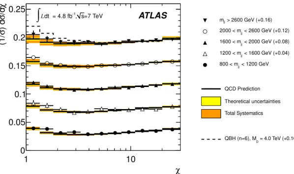
The observed χ distributions normalised to unit area are shown in figure 2 for several mjj bins, defined by boundaries at 800, 1200, 1600, 2000, and 2600 GeV. The highest bin

includes all dijet events with mjj > 2.6 TeV. The dijet mass bins are chosen to ensure

sufficient entries in each mass bin. From the lowest dijet mass bin to the highest bin, the number of events are: 13642, 4132, 35250, 28462, 2706, and the corresponding integrated luminosities are 5.6 pb−1_{, 19.2 pb}−1_{, 1.2 fb}−1_{, 4.8 fb}−1 _{and 4.8 fb}−1_{. The yield for all}

mjj < 2000 GeV is reduced due to the usage of prescaled triggers, and for mjj > 2000 GeV

by the falling cross section.

The χ distributions are compared to the predictions from QCD, which include all systematic uncertainties, and the signal predictions of one particular NP model, a quantum black hole (QBH) scenario with a quantum gravity mass scale of 4.0 TeV and six extra dimensions [7,8].

Pseudo-experiments are used to convolve statistical, systematic and theoretical uncer-tainties on the QCD predictions, as has been done in previous studies of this type [18]. The primary sources of theoretical uncertainty are NLO QCD renormalisation and factorisation scales, and PDF uncertainties. The QCD scales are varied by a factor of two independently around their nominal values, which are set to the mean pT of the leading jets, while the

PDF uncertainties are determined using CT10 NLO PDF error sets [52]. The resulting bin-wise uncertainties for the cross-section normalised χ distributions can be as high as 8% for the combined NLO QCD scale variations and are typically below 1% for the PDF uncertainties. These theoretical uncertainties are convolved with the JES uncertainty and applied to all MC angular distributions. Other experimental uncertainties such as those

JHEP01(2013)029

∫

Figure 2. The χ distributions for all dijet mass bins. The QCD predictions are shown with theo-retical and total systematic uncertainties (bands), as well as the data with statistical uncertainties. The dashed line is the prediction for a QBH signal for MD = 4.0 TeV and n = 6 in the highest

mass bin. The distributions have been offset by the amount shown in the legend to aid in visually comparing the shapes in each mass bin.

due to pile-up and to the jet energy and angular resolutions have been investigated and found to be negligible. The JES uncertainties are largest at low χ and are as small as 5% for the lowest dijet mass bin but increase to above 15% for the highest bin. Variations based on the resulting systematic uncertainties are used in generating statistical ensembles for the estimation of p-values when comparing QCD predictions to data.

A statistical analysis is performed on each of the five χ distributions to test the overall consistency between data and QCD predictions. A binned log-likelihood is calculated for each distribution assuming that the sample consists only of QCD dijet production. The expected distribution of this likelihood is then determined using pseudo-experiments drawn from the QCD MC sample and convolved with the systematic uncertainties as discussed above. Finally the p-value is defined as the probability of obtaining a log-likelihood value less than the value observed in data.

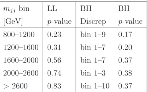
The p-values determined from the observed likelihoods are shown in table 1. These indicate that there is no statistically significant evidence for new phenomena in the χ dis-tributions, and that these distributions are in reasonable agreement with QCD predictions. As with the dijet resonance analysis, the BumpHunter algorithm is applied to the five χ distributions separately, in this case to test for the presence of features that might indicate disagreement with the QCD prediction. The results are shown in table 1. In this particular application, the BumpHunter is required to start from the first χ bin, and the excess must be at least three bins wide. For each of the bin combinations, the binomial p-value for observing the data given the QCD-background-only hypothesis is calculated. The bin sequence with the smallest binomial p-value is listed in table 1. Statistical and

JHEP01(2013)029

mjj bin LL BH BH

[GeV] p-value Discrep p-value

800–1200 0.23 bin 1–9 0.17

1200–1600 0.31 bin 1–7 0.20

1600–2000 0.56 bin 1–7 0.37

2000–2600 0.74 bin 1–3 0.38

> 2600 0.83 bin 1–10 0.37

Table 1. Comparing χ distributions to QCD predictions. The abbreviations in the first line of the table stand for “log-likelihood” (LL), and “BumpHunter” (BH). The second line labels the “p-values” (p-value) and the “most discrepant region” (Discrep).

systematic uncertainties, and look-elsewhere effects, are included using pseudo-experiments drawn from the QCD background. For each of the pseudo-experiments the most discrepant bin combination is found and its p-value is used to construct the expected binomial p-value distribution. The final BumpHunter p-value is then defined as the probability of finding a binomial p-value as extreme as the one observed in data. The p-values listed in the last column of table1indicate that the data are consistent with the QCD prediction in all five mass bins.

In addition, the BumpHunter algorithm is applied to all χ distributions at once, which increases the effect of the correction for the look-elsewhere effect. The most discrepant region in all distributions is in bins 1–9 of the 800–1200 GeV mass distribution. The resulting p-value, including the look-elsewhere effect, is now 0.43, again indicating good agreement with QCD predictions.

8 Comparing the Fχ(mjj) distribution to the QCD prediction

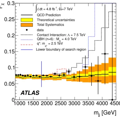
The observed Fχ(mjj) data distribution is shown in figure 3, where it is compared to the

QCD prediction, which includes all systematic uncertainties. Also shown in the figure is the expected behaviour of Fχ(mjj) if a contact interaction with the compositeness scale

Λ = 7.5 TeV were present [53,54]. Furthermore the predictions for an excited quark with a mass of 2.5 TeV and a QBH signal with MD = 4.0 TeV are shown. The blue vertical line

at 1.8 TeV included in figure 3indicates the mass boundary above which the search phase of the analysis is performed, as explained below.

The observed Fχ(mjj) distribution is obtained by forming the finely-binned mjj

dis-tributions for Ncentral and Ntotal — the “numerator” and “denominator” distributions

of Fχ(mjj) — separately and taking the ratio. The handling of systematic

uncertain-ties, including JES, PDF and scale uncertainuncertain-ties, uses a procedure similar to that for the χ distributions.

Two statistical tests are applied to the high-mass region to determine whether the data are compatible with the QCD prediction. The first test uses a binned likelihood, which includes the systematic uncertainties, and is constructed assuming the presence of QCD

JHEP01(2013)029

[GeV]

m

1000 1500 2000 2500 3000 3500 4000 4500

F

0

0.05

0.1

0.15

0.2

0.25

0.3

ATLAS

∫

Lower boundary of search region

Figure 3. The Fχ(mjj) distribution in mjj. The QCD prediction is shown with theoretical and

total systematic uncertainties (bands), and data (black points) with statistical uncertainties. The blue vertical line indicates the lower boundary of the search region for new phenomena. Various expected new physics signals are shown: a contact interaction with Λ = 7.5 TeV, an excited quark with mass 2.5 TeV and a QBH signal with MD= 4.0 TeV.

processes only. The p-value calculated from this likelihood is 0.38, indicating that these data are in agreement with the QCD prediction.

The second test consists of applying the BumpHunter and TailHunter algorithms [36, 37] to the Fχ(mjj) distributions, including systematic uncertainties and assuming

binomial statistics. For this test only data with dijet masses above 1.8 TeV, associated with the single unprescaled trigger, are used to obtain a high sensitivity at high mass and to avoid diluting the test with the large number of low-mass bins. The test scans the data using windows of varying widths and identifies the window with the largest excess of events with respect to the background. The BumpHunter finds the most discrepant interval to be from 1.80 TeV to 2.88 TeV, with a p-value of 0.20. The TailHunter finds the most discrepant interval to be from 1.80 TeV onwards, with a p-value of 0.21. The p-values indicate that there is no significant excess in the data .

9 Simulation of hypothetical new phenomena

In the absence of any significant signals indicating the presence of phenomena beyond QCD, Bayesian 95% credibility level (CL) limits are determined for a number of NP hypotheses. The following models have been described in detail in previous ATLAS dijet studies [17,

JHEP01(2013)029

scalars (s8) [6], and quantum black holes (QBH) [7,8]. Two models of new phenomena are added to the current analysis: heavy W bosons (W′_{) with SM couplings [55–57], and string}

resonances (SR) [9–12]. Contact interactions and QBH appear as slowly rising effects in mjj, while the other hypotheses produce localised excesses.

A number of these NP models are available in the Pythia 6 event generator. In these cases, the corresponding MC samples are generated using the AUET2B LO** tune and the MRSTMCal PDF. For NP models provided by other event generators, with other PDFs, partons originating from the initial two-parton interaction are used as input to Pythia which performs parton showering and the remaining event generation steps. In all cases, the renormalisation and factorisation scales are set to the mean pT of the leading jets.

The quark contact interaction, CI, is used to model the appearance of kinematic prop-erties that characterise quark compositeness. In the current analysis, only destructive interference is studied, but constructive interference is expected to give less conservative limits. Pythia 6 is used to create MC event samples for distinct values of the composite-ness scale, Λ.

Excited quarks, q∗_{, a possible manifestation of quark compositeness, are also simulated}

in all decay modes with Pythia 6 for selected values of the q∗ _{mass. Excited quarks}

are assumed to decay to common quarks via standard model couplings, leading to gluon emission approximately 83% of the time. Recent studies comparing this benchmark model to the same excited quark model in Pythia 8 show that the q∗_m

jjdistribution in Pythia 8

is significantly broader than that in Pythia 6. The Pythia authors have identified a long-standing misapplication of QCD pT-ordered final state radiation (FSR) vetoing in

Pythia 6, which is resolved in Pythia 8. The q∗ _m

jj distributions from Pythia 6 can

be brought into close correspondence with Pythia 8 by setting the Pythia 6 MSTJ(47) parameter to zero, restoring the correct behaviour for final state radiation. The resulting widening of the peak affects the search sensitivity and exclusion limits. The q∗_{MC samples}

used in the current studies are generated using both the default and corrected Pythia 6 settings, to determine the impact on the q∗ _{exclusion limit.}

The colour octet scalar model, s8, is a typical example of possible exotic coloured resonances decaying to two gluons. MadGraph 5 [58] with the CTEQ6L1 PDF [59] is employed to generate parton-level event samples at leading-order approximation for a selection of s8 masses, which are used as input to Pythia 6.

A model for quantum black holes, QBH, that decay to two jets is simulated using BlackMax [60] with the CT10 PDF to produce a simple two-body final state scenario of quantum gravitational effects at the reduced Planck Scale MD, with n = 6 extra spatial

dimensions. The QBH model is used as a benchmark to represent any quantum gravita-tional effect that produces events containing dijets. Event samples for selected values of MD are used as input to Pythia for further processing.

The first new NP phenomenon used in the current dijet analysis, the production of heavy charged gauge bosons, W′_{, has been sought in events containing a charged lepton}

(electron or muon) and a neutrino [56,57], but no evidence has been found. In the current studies, dijet events are searched for the decays of W′ _{to q ¯q}′_{. The specific model used in}

JHEP01(2013)029

this study [55] assumes that the W′_{has V-A SM couplings but does not include interference}

between the W′ _{and the W . The W}′ _{signal sample is generated with the Pythia 6 event}

generator. Instead of the LO cross section values, the NNLO electroweak-corrected cross section values [57, 61–63] calculated using the MSTW2008 PDF [64], are used in this analysis. For a given W′ _{mass, the width of the resonance in m}

jj is very similar to that of

the q∗_{, and the angular distribution peaks at low χ. The limit analysis for this W}′ _model

includes the branching ratio to the chosen q ¯q′ _{final state and, for each simulated mass, this}

fraction is taken from Pythia 6.

The second new NP model considered, string resonances (SR), results from excitations of quarks and gluons at the string level [9–12]. The dominant decay mode is to qg, and the SR model described in ref. [11] is implemented in the CalcHEP generator [65] with the MRSTMCal PDF. As with other models, MC samples are created for selected values of the mass parameter, mSR, by passing the CalcHEP output at parton level to Pythia 6.

All MC signal samples are passed through fast detector simulation using ATLFAST 2.0, except for string resonances, which are fully simulated using Geant4.

10 Limits on new resonant phenomena from the mjj distribution

For each NP process under study, Monte Carlo samples have been simulated at a number of selected mass points, mNP. The Bayesian method documented in ref. [22] is applied to

data at these same mass points to set a 95% CL limit on the cross section times acceptance, σ × A, for the NP signal as a function of mNP, using a prior constant in signal strength.

The limit on σ × A from data is interpolated between mass points to create a continuous curve in mjj. The exclusion limit on the mass (or energy scale) of the given NP signal

occurs at the value of mjj where the limit on σ ×A from data is the same as the theoretical

value, which is derived by interpolation between the generated mass values.

This form of analysis is applicable to all resonant phenomena where the NP cou-plings are strong compared to the scale of perturbative QCD at the signal mass, so that interference with QCD terms can be neglected. The acceptance calculation includes all re-construction steps and analysis cuts described in section4. For all resonant models except for the W′_{, all decay modes have been simulated so that the branching ratio into dijets}

is implicitly included in the acceptance through the analysis selection. For the W′ _model,

only dijet final states have been simulated, and the branching ratio is included in the cross section instead of in the acceptance.

The effects of systematic uncertainties due to luminosity, acceptance, and jet energy scale are included. The luminosity uncertainty for the 2011 data is 3.9% [24] and is com-bined in quadrature with the acceptance uncertainty. The correlated systematic uncertain-ties corresponding to the 14 JES nuisance parameters are added in quadrature and repre-sented by a single nuisance parameter which shifts the resonance mass peaks by less than 4%. The background parameterisation uncertainty is taken from the fit results, as described in ref. [22]. The effect of the jet energy resolution uncertainty is found to be negligible.

These uncertainties are incorporated into the fit by varying all sources according to Gaussian probability distributions and convolving them with the posterior probability

dis-JHEP01(2013)029

Observed 95% CL upper limit Expected 95% CL upper limit 68% and 95% bands ATLAS -1 = 4.8 fb dt L ∫ = 7 TeV s

(a) Excited-quark model.

Mass [GeV] 2000 3000 4000 [pb] xA × σ -2 10 -1 10 1 10 2 10 s8

Observed 95% CL upper limit Expected 95% CL upper limit 68% and 95% bands ATLAS -1 = 4.8 fb dt L ∫ = 7 TeV s

(b) Colour scalar octet model.

Figure 4. The 95% CL upper limits on σ × A as a function of particle mass (black filled circles) using mjj. The black dotted curve shows the 95% CL upper limit expected in the absence of

any resonance signal, and the green and yellow bands represent the 68% and 95% contours of the expected limit, respectively. Theoretical predictions of σ × A are shown (dashed) in (a) for excited quarks, and in (b) for colour octet scalars. For a given NP model, the observed (expected) limit occurs at the crossing of the dashed σ × A curve with the observed (expected) 95% CL upper limit curve.

tribution. Credibility intervals are then calculated numerically from the resulting convo-lutions. No uncertainties are associated with the theoretical model, as in each case the NP model is a benchmark that incorporates a specific choice of model parameters, PDF set, and MC tune. Previous ATLAS studies using the q∗ _{theoretical prediction [22] showed}

that the variation among three different choices of MC tune and PDF set was less than 4% for the expected limits.

The resulting limits for excited quarks, based on the corrected Pythia 6 samples (as explained in section 9), are shown in figure 4(a)_{. The acceptance A ranges from 40% to}

51% for mq∗ between 1.2 TeV and 4.0 TeV, and is never lower than 46% for masses above

1.4 TeV. The largest reduction in acceptance arises from the rapidity selection criteria. The expected lower mass limit at 95% CL for q∗ _{is 2.94 TeV, and the observed limit is}

2.83 TeV. For comparison, this limit has also been determined using Pythia 6 samples with the default q∗ _{settings, leading to narrower mass peaks. The expected limit determined}

from these MC samples is 0.1 TeV higher than the limit based on the corrected samples. This shift is an approximate indicator of the fractional correction that is expected when comparing the current ATLAS results to all previous analyses that found q∗ _{mass limits}

using Pythia 6 and pT-ordered final state radiation without corrections, including all

previous ATLAS results.

The limits for colour octet scalars are shown in figure 4(b). The expected mass limit at 95% CL is 1.97 TeV, and the observed limit is 1.86 TeV. For this model the acceptance values vary between 34% and 48% for masses between 1.3 TeV and 4.0 TeV.

JHEP01(2013)029

Observed 95% CL upper limit Expected 95% CL upper limit 68% and 95% bands ATLAS -1 = 4.8 fb dt L ∫ = 7 TeV s

(a) Heavy charged gauge bosons, W′_.

Mass [GeV] 2000 3000 4000 5000 [pb] xA × σ -3 10 -2 10 -1 10 1 10 2 10 String Resonance

Observed 95% CL upper limit Expected 95% CL upper limit 68% and 95% bands ATLAS -1 = 4.8 fb dt L ∫ = 7 TeV s (b) String resonances, SR.

Figure 5. In (a), 95% CL upper limits on σ × A × BR as a function of particle mass (black filled circles) from mjj analysis are shown for heavy gauge bosons, W′. The black dotted curve

shows the 95% CL upper limit expected in the absence of any resonance signal, and the green and yellow bands represent the 68% and 95% contours of the expected limit, respectively. The observed (expected) limit occurs at the crossing of the dashed theoretical σ ×A× BR curve with the observed (expected) 95% CL upper limit curve. In (b), 95% CL upper limits on σ × A are shown for string resonances, SR, with the equivalent set of contours for this model, and the same method of limit determination.

The limits for heavy charged gauge bosons, W′_{, are shown in figure 5(a). For this}

model, only final states with dijets have been simulated. The branching ratio, BR, to the studied q ¯q′ _{final state varies little with mass and is 0.75 for m}

W′ values of 1.1 TeV to

3.6 TeV, and the acceptance ranges from 29% to 36%. The expected mass limit at 95% CL is 1.74 TeV, and the observed limit is 1.68 TeV. This is the first time that an ATLAS limit on W′ _{production is set using the dijet mass distribution. Searches for leptonic decays of}

the W′ _{are however expected to be more sensitive.}

The W′ _{hypothesis used in the current study assumes SM couplings to quarks. If a}

similar model were to predict stronger couplings, for example, figure 5(a) could be used to estimate the new mass limit by shifting the theoretical curve upward by the ratio of the squared couplings. Alternately, the current limit on W′ _{decaying to dijets could be}

of interest for comparison with leptophobic W′ _{models, where all final states would be}

hadronic [66–69].

The limits for string resonances are shown in figure 5(b). The SR acceptance ranges from 45% to 48% for masses varying from 2.0 TeV to 5.0 TeV. The expected mass limit at 95% CL is 3.47 TeV, and the observed limit is 3.61 TeV.

Tables with acceptance values and limits for all models discussed here can be found in appendix A.

JHEP01(2013)029

[GeV]

Mass, m

[pb]

xA

×

σ

95

%

C

L

Li

m

it

on

ATLAS

∫

Figure 6. The 95% CL upper limits on σ × A for a simple Gaussian resonance decaying to dijets as a function of the mean mass, mG, for three values of σG/mG, taking into account both statistical

and systematic uncertainties.

11 Model-independent limits on dijet resonance production

As in previous dijet resonance analyses, limits on dijet resonance production are deter-mined here using a Gaussian resonance shape hypothesis. Limits are set for a collection of hypothetical signals that are assumed to be Gaussian-distributed in mjj with means

(mG) ranging from 1.0 TeV to 4.0 TeV and with standard deviations (σG) from 7% to 15%

of the mean.

Systematic uncertainties are treated using the same methods as applied in the model-dependent limit setting described above. The only difference between the Gaussian analysis and the standard analysis is that the decay of the dijet final state is not simulated. In place of this, it is assumed that the dijet signal mass distribution is Gaussian in shape, and the JES uncertainty is modelled as an uncertainty of 4% in the central value of the Gaussian signal. This approach has been validated by shifting the energy of all jets in Pythia 6 signal templates by their JES uncertainty and evaluating the relative shift of the mass peak. The resulting limits on σ×A for the Gaussian template model are shown in figure6and detailed in table2. These results may be utilised to set limits on NP models beyond those considered in the current studies, under the condition that their signal shape approaches a Gaussian distribution after applying the kinematic selection criteria on y∗_{, m}

JHEP01(2013)029

leading jets (section 4). The acceptance should include the branching ratio of the particle decaying into dijets and the physics selection efficiency. The ATLAS mjj resolution is

about 5%, hence NP models with a width smaller than 7% should be compared to the 7% column of table2. Models with a greater width should use the column that best matches their width. A detailed description of the recommended procedure, including the treatment of detector resolution effects, is given in ref. [23].

12 Limits on CI and QBH from the χ distributions

The χ distribution in the highest mass bin of figure2 is used to set 95% CL limits on two NP hypotheses, CI and QBH.

In the contact interaction analysis, four MC samples of QCD production modified by a contact interaction are created for values of Λ ranging from 4.0 TeV to 10.0 TeV. For the CI distributions, QCD K-factors are applied to the QCD-only component of the cross section, as follows: before normalising the χ-distributions to unit area, the LO QCD part of the cross section, determined from a QCD-only simulation sample, is replaced by the QCD cross section corrected for NLO effects.

Using the QCD distribution and the finite set of MC CI distributions, each χ-bin is fit as function of Λ against a four-parameter interpolation function,3 _{allowing for a smooth}

integration of the posterior probability density functions over Λ. From the signal fits, a posterior probability density is constructed as a function of Λ. The systematic uncertain-ties described in section 7 are convolved with the posterior distribution through pseudo-experiments drawn from the NP hypotheses. For the expected limit, pseudo-pseudo-experiments are performed on the QCD background and used as pseudo-data.

This analysis sets a 95% CL lower limit on Λ at 7.6 TeV with an expected limit of 7.7 TeV. The observed posterior probability density function is shown in figure7.

To test the sensitivity of the CI limit to the choice of prior, this analysis is repeated for a constant prior in 1/Λ2_{, which has been used in previous publications. As anticipated, the}

expected limit is less conservative, increasing by 0.40 TeV. Since the constant prior in 1/Λ4

more accurately follows the cross section predicted for CI, the 1/Λ2 _{result is not reported}

in the final results of the current studies.

The second model is QBH with n = 6 and with a constant prior in 1/M4

D, which is for

n = 6 proportional to the cross section. Similarly to what is done for CI, the QCD sample, together with a set of eleven QBH samples with MD ranging from 2.0 TeV to 6.0 TeV,

is fit to the same smooth function in every χ-bin to enable integration of the posterior probability density functions over MD. The expected and observed 95% CL lower limits

on MD are 4.20 TeV and 4.11 TeV, respectively.

13 Limits on new resonant phenomena from the Fχ(mjj) distribution

The Bayesian approach employed to set exclusion limits on new resonant phenomena with the dijet mass spectrum may be applied to the Fχ(mjj) distribution (see figure 3),

pro-3_{The fitting function is f (x) = p}

JHEP01(2013)029

Observed 95% CL upper limits on σ × A [pb] mG [GeV] σG/mG= 7% σG/mG= 10% σG/mG= 15% 1000 0.66 0.67 0.61 1050 0.56 0.58 0.57 1100 0.44 0.51 0.41 1150 0.28 0.37 0.26 1200 0.18 0.22 0.21 1250 0.14 0.16 0.18 1300 0.11 0.12 0.16 1350 0.093 0.11 0.16 1400 0.083 0.11 0.15 1450 0.084 0.10 0.17 1500 0.090 0.11 0.17 1550 0.087 0.12 0.20 1600 0.090 0.11 0.18 1650 0.082 0.11 0.17 1700 0.079 0.11 0.17 1750 0.078 0.10 0.15 1800 0.069 0.097 0.13 1850 0.066 0.091 0.12 1900 0.061 0.075 0.11 1950 0.054 0.068 0.095 2000 0.049 0.058 0.085 2100 0.035 0.047 0.073 2200 0.029 0.040 0.066 2300 0.027 0.036 0.054 2400 0.024 0.031 0.044 2500 0.020 0.027 0.032 2600 0.017 0.021 0.021 2700 0.014 0.017 0.013 2800 0.012 0.012 0.0084 2900 0.0087 0.0075 0.0063 3000 0.0062 0.0052 0.0047 3200 0.0030 0.0032 0.0032 3400 0.0021 0.0021 0.0021 3600 0.0015 0.0016 0.0016 3800 0.0012 0.0012 0.0013 4000 0.0010 0.0010 0.0011

Table 2. The 95% CL upper limit on σ × A [pb] for the Gaussian model. The symbols mG and

JHEP01(2013)029

]

[1/TeV

Λ

1/

0

0.2

0.4

0.6

0.8

1

10

×

pdf value

0

1

2

3

4

5

10

×

ATLAS

∫

Figure 7. Observed posterior probability density function as function of 1/Λ4

for the CI model. The coloured area shows the 95% area, and the blue dashed line denotes the 95% CL limit.

vided that the NP models under consideration do not include interference with QCD. Unlike the mjj resonance analysis, the background prediction is based on the QCD MC

samples processed through detector simulation and corrected for NLO effects. The like-lihood is constructed from two mjj distributions and their associated uncertainties, one

distribution being the numerator spectrum of the Fχ(mjj) distribution and the other

be-ing the denominator. Here too, pseudo-experiments are used to convolve all systematic uncertainties, which in this case include the JES uncertainties, and the PDF and scale uncertainties associated with the QCD prediction.

Figure8shows the limits expected and observed from data on the production cross sec-tion σ times the acceptance A, along with theoretical predicsec-tions for the QBH model [7,8], for n ranging from two to seven. For this model, generator-level studies have shown that the acceptance does not depend on the number of extra dimensions within this range. There-fore only the QBH MC sample for n = 6 has been processed through the ATLFAST 2.0 detector simulation, and the acceptance calculated from this sample is used for all values of n. The acceptance is close to 90% for all MD values. The resulting 95% CL exclusion

limits for the number of extra dimensions n ranging from 2 to 7 are shown in table3. The same analysis is applied to detect resonances in Fχ(mjj) due to excited quarks.

With an acceptance close to 90% for all masses this analysis sets a 95% CL lower limit on mq∗ at 2.75 TeV with an expected limit of 2.85 TeV.

JHEP01(2013)029

[GeV]

M

2000

3000

4000

5000

[pb]

xA

×

σ

10

10

10

10

1

10

10

10

10

10

ATLAS

Observed 95% CL upper limit Expected 95% CL upper limit 68% band 95% band QBH n=5 QBH n=6 QBH n=7 =7 TeV s , -1 dt = 4.8 fb L

∫

Figure 8. The 95% CL upper limits on σ × A as function of the reduced Planck mass MD of

the QBH model using Fχ(mjj) (black filled circles). The black dotted curve shows the 95% CL

upper limit expected from Monte Carlo, and the green and yellow bands represent the 68% and 95% contours of the expected limit, respectively. Theoretical predictions of σ × A are shown for various numbers of extra dimensions.

n extra Expected Observed

dimensions limit [TeV] limit [TeV]

2 3.85 3.71 3 3.99 3.84 4 4.07 3.92 5 4.12 3.99 6 4.16 4.03 7 4.19 4.07

Table 3. Lower limits at 95% CL on MD of the QBH model with n = 2 to 7 extra dimensions.

14 Limits on CI from the Fχ(mjj) distribution

As was done previously with the ATLAS 2010 data sample [22], the Fχ(mjj) distribution

(see figure3) is used in the current study to set limits on quark contact interactions. The procedure is very similar to the one used for limits obtained with χ discussed in section 12. MC samples of QCD production modified by a contact interaction are created for values of Λ ranging from 4.0 TeV to 10.0 TeV. For the CI distributions, QCD K-factors are applied to the QCD-only components of the numerator and denominator of Fχ(mjj)

JHEP01(2013)029

separately. This is done by subtracting the LO QCD cross section and adding the QCD cross section corrected for NLO effects.

Simulated Fχ(mjj) distributions are statistically smoothed by a fit in mjj. For the

pure QCD sample (corresponding to Λ = ∞), a second-order polynomial is used, while for the MC distributions with finite Λ, a Fermi function is added to the polynomial, which gives a good representation of the onset of contact interactions.

Next, all mjj bins of the MC Fχ(mjj) distributions are interpolated in Λ using the same

four-parameter interpolation function used for the χ analysis, creating a smooth predicted Fχ(mjj) surface as a function of mjj and Λ. This surface enables integration in mjj vs. Λ

for continuous values of Λ.

Pseudo-experiments are then employed to construct a posterior probability, assuming a prior that is flat in 1/Λ4_{. This analysis sets a 95% CL lower limit on Λ at 7.6 TeV with}

an expected limit of 7.7 TeV.

15 Conclusions

Dijet mass and angular distributions have been measured by the ATLAS experiment over a large angular range and spanning dijet masses up to approximately 4.0 TeV, using 4.8 fb−1

of pp collision data at √s = 7 TeV. No resonance-like features have been observed in the dijet mass spectrum, and all angular distributions are consistent with QCD predictions. This analysis places limits on a variety of hypotheses for physics phenomena beyond the Standard Model, as summarised in table 4.

For√s = 7 TeV pp collisions at the LHC, the integrated luminosity used in the current studies represents a substantial increase over that available in previously published ATLAS dijet searches. Table5 lists the previous and current expected limits from ATLAS studies using dijet analyses for three benchmark models: excited quarks, colour octet scalars, and contact interactions with destructive interference. The increase in the excited quark mass limit would have been greater by 0.10 TeV had there not been the long-standing problem with the default Pythia 6 q∗ _{model, discussed in earlier sections.}

For 2012 running, the collision energy of the LHC has been raised from 7 TeV to 8 TeV. The higher energy, and the associated rise in parton luminosity, will increase search sensitivities and the possibility of discoveries. The current 2011 analysis provides a reference for the study of energy-dependent effects once the 2012 data set has been analysed. Acknowledgments

We thank Noriaki Kitazawa for the string resonance amplitude calculations and event samples.

We thank CERN for the very successful operation of the LHC, as well as the support staff from our institutions without whom ATLAS could not be operated efficiently.

We acknowledge the support of ANPCyT, Argentina; YerPhI, Armenia; ARC, Aus-tralia; BMWF and FWF, Austria; ANAS, Azerbaijan; SSTC, Belarus; CNPq and FAPESP, Brazil; NSERC, NRC and CFI, Canada; CERN; CONICYT, Chile; CAS, MOST and

JHEP01(2013)029

Model and Analysis Strategy 95% CL Limits [TeV]

Expected Observed

Excited quark, mass of q∗

Resonance in mjj 2.94 2.83

Resonance in Fχ(mjj) 2.85 2.75

Colour octet scalar, mass of s8

Resonance in mjj 1.97 1.86

Heavy W boson, mass of W′

Resonance in mjj 1.74 1.68

String resonances, scale of SR

Resonance in mjj 3.47 3.61

Quantum Black Hole for n = 6, MD

Fχ(mjj) 4.16 4.03

χ , mjj > 2.6 TeV 4.20 4.11

Contact interaction, Λ, destructive interference

Fχ(mjj) 7.7 7.6

χ , mjj > 2.6 TeV 7.7 7.6

Table 4. The 95% CL lower limits on the masses and energy scales of the models examined in this study. All limit analyses are Bayesian, with statistical and systematic uncertainties included. For each NP hypothesis, the result corresponding to the highest expected limit is the result quoted in the abstract.

New Phenomenon 36 pb−1 _{[22] 1.0 fb}−1 _{[23] 4.8 fb}−1_current

Resonance in mjj

Excited quark, mass of q∗ _{2.07 2.81 2.94}

Colour octet scalar, mass of s8 — 1.77 1.97

Angular distribution in χ

Contact interaction, Λ 5.4 — 7.7

Table 5. ATLAS previous and current expected 95% CL upper limits [TeV] on new phenomena. The current expected limit for q∗ _{cannot be compared directly to the two previous limits since}

they employed Pythia 6 samples with an error in the simulation of final state radiation. Had such samples been used in the current analysis, the expected q∗ _{limit would be 0.10 TeV higher.}

NSFC, China; COLCIENCIAS, Colombia; MSMT CR, MPO CR and VSC CR, Czech Re-public; DNRF, DNSRC and Lundbeck Foundation, Denmark; EPLANET, ERC and NSRF, European Union; IN2P3-CNRS, CEA-DSM/IRFU, France; GNSF, Georgia; BMBF, DFG, HGF, MPG and AvH Foundation, Germany; GSRT and NSRF, Greece; ISF, MINERVA, GIF, DIP and Benoziyo Center, Israel; INFN, Italy; MEXT and JSPS, Japan; CNRST, Mo-rocco; FOM and NWO, Netherlands; BRF and RCN, Norway; MNiSW, Poland; GRICES and FCT, Portugal; MERYS (MECTS), Romania; MES of Russia and ROSATOM,

Rus-JHEP01(2013)029

sian Federation; JINR; MSTD, Serbia; MSSR, Slovakia; ARRS and MVZT, Slovenia; DST/NRF, South Africa; MICINN, Spain; SRC and Wallenberg Foundation, Sweden; SER, SNSF and Cantons of Bern and Geneva, Switzerland; NSC, Taiwan; TAEK, Turkey; STFC, the Royal Society and Leverhulme Trust, United Kingdom; DOE and NSF, United States of America.

The crucial computing support from all WLCG partners is acknowledged gratefully, in particular from CERN and the ATLAS Tier-1 facilities at TRIUMF (Canada), NDGF (Denmark, Norway, Sweden), CC-IN2P3 (France), KIT/GridKA (Germany), INFN-CNAF (Italy), NL-T1 (Netherlands), PIC (Spain), ASGC (Taiwan), RAL (UK) and BNL (USA) and in the Tier-2 facilities worldwide.

A Limits on new resonant phenomena from the mjj distribution

A.1 Excited quarks

mq∗ [GeV] Observed Expected Expected ±1σ Expected ±2σ A

1000 1.43 0.55 0.36/1.064 0.31/1.58 0.299 1200 0.30 0.36 0.27/0.66 0.23/0.99 0.403 1400 0.16 0.22 0.17/0.35 0.14/0.52 0.459 1600 0.16 0.15 0.12/0.25 0.098/0.37 0.481 1800 0.16 0.10 0.079/0.16 0.065/0.24 0.497 2000 0.12 0.071 0.054/0.11 0.043/0.16 0.501 2250 0.064 0.045 0.034/0.070 0.027/0.10 0.505 2500 0.050 0.032 0.023/0.050 0.018/0.071 0.511 2750 0.032 0.023 0.016/0.036 0.013/0.051 0.499 3000 0.017 0.016 0.012/0.024 0.0094/0.034 0.500 3250 0.0081 0.011 0.0086/0.017 0.0069/0.024 0.505 3500 0.0056 0.0081 0.0062/0.012 0.0049/0.016 0.499 3750 0.0041 0.0063 0.0047/0.0090 0.0037/0.013 0.493 4000 0.0034 0.0049 0.0036/0.0070 0.0028/0.010 0.484

Table 6. The 95% CL upper limit on σ × A [pb] for excited quarks, q∗_.

A.2 Colour octet scalars

ms8 [GeV] Observed Expected Expected ±1σ Expected ±2σ A

1300 0.40 0.68 0.38/1.45 0.31/2.20 0.339 1500 0.27 0.38 0.27/0.75 0.23/1.18 0.405 1700 0.24 0.27 0.20/0.52 0.17/0.79 0.443 2000 0.33 0.16 0.12/0.29 0.099/0.43 0.467 2500 0.17 0.084 0.059/0.14 0.049/0.21 0.484 3000 0.097 0.062 0.042/0.11 0.034/0.17 0.441 3500 0.034 0.049 0.036/0.079 0.030/0.12 0.390 4000 0.035 0.048 0.038/0.073 0.032/0.11 0.357

JHEP01(2013)029

A.3 Heavy W boson

mW′ [GeV] Observed Expected Expected ±1σ Expected ±2σ A

1100 0.65 0.46 0.32/0.88 0.27/1.30 0.286 1200 0.29 0.35 0.26/0.62 0.22/0.90 0.314 1400 0.15 0.21 0.16/0.33 0.13/0.48 0.345 1600 0.15 0.14 0.11/0.23 0.094/0.33 0.358 1800 0.13 0.099 0.077/0.16 0.063/0.23 0.353 2000 0.12 0.072 0.055/0.11 0.045/0.16 0.341 2400 0.065 0.042 0.031/0.064 0.025/0.090 0.293

Table 8. The 95% CL upper limit on σ × A × BR [pb] for Heavy W bosons, W′_.

A.4 String resonances

mSR [GeV] Observed Expected Expected ±1σ Expected ±2σ A

2000 0.094 0.059 0.041/0.080 0.032/0.12 0.449 2500 0.036 0.026 0.017/0.034 0.013/0.048 0.447 3000 0.012 0.012 0.0077/0.016 0.0061/0.022 0.452 3500 0.0041 0.0059 0.0036/0.0069 0.0028/0.010 0.464 4000 0.0021 0.0032 0.0020/0.0038 0.0016/0.0058 0.458 4500 0.0016 0.0023 0.0016/0.0029 0.0013/0.0040 0.478 5000 0.0013 0.0019 0.0012/0.0024 0.0010/0.0034 0.482

Table 9. The 95% CL upper limit on σ × A [pb] for string resonances, SR.

Open Access. This article is distributed under the terms of the Creative Commons Attribution License which permits any use, distribution and reproduction in any medium, provided the original author(s) and source are credited.

References

[1] U. Baur, I. Hinchliffe and D. Zeppenfeld, Excited quark production at hadron colliders,

Int. J. Mod. Phys.A 2 (1987) 1285[INSPIRE].

[2] U. Baur, M. Spira and P. Zerwas, Excited quark and lepton production at hadron colliders,

Phys. Rev.D 42 (1990) 815[INSPIRE].

[3] P.H. Frampton and S.L. Glashow, Chiral color: an alternative to the standard model,

Phys. Lett.B 190 (1987) 157[INSPIRE].

[4] P.H. Frampton and S.L. Glashow, Unifiable chiral color with natural

Glashow-Iliopoulos-Maiani mechanism,Phys. Rev. Lett.58 (1987) 2168[INSPIRE].

[5] J. Bagger, C. Schmidt and S. King, Axigluon production in hadronic collisions,

Phys. Rev.D 37 (1988) 1188 [INSPIRE].

[6] T. Han, I. Lewis and Z. Liu, Colored resonant signals at the LHC: largest rate and simplest topology,JHEP 12 (2010) 085 [arXiv:1010.4309] [INSPIRE].

JHEP01(2013)029

[7] P. Meade and L. Randall, Black holes and quantum gravity at the LHC,JHEP 05 (2008) 003

[arXiv:0708.3017] [INSPIRE].

[8] L.A. Anchordoqui, J.L. Feng, H. Goldberg and A.D. Shapere, Inelastic black hole production and large extra dimensions,Phys. Lett.B 594 (2004) 363[hep-ph/0311365] [INSPIRE].

[9] S. Cullen, M. Perelstein and M.E. Peskin, TeV strings and collider probes of large extra dimensions,Phys. Rev.D 62 (2000) 055012[hep-ph/0001166] [INSPIRE].

[10] L.A. Anchordoqui, H. Goldberg, S. Nawata and T.R. Taylor, Jet signals for low mass strings at the LHC,Phys. Rev. Lett.100 (2008) 171603[arXiv:0712.0386] [INSPIRE].

[11] L.A. Anchordoqui et al., LHC phenomenology for string hunters,

Nucl. Phys.B 821 (2009) 181[arXiv:0904.3547] [INSPIRE].

[12] N. Kitazawa, A closer look at string resonances in dijet events at the LHC,

JHEP 10 (2010) 051[arXiv:1008.4989] [INSPIRE].

[13] UA1 collaboration, G. Arnison et al., Angular distributions and structure functions from two jet events at the CERN SPSp¯p collider,Phys. Lett.B 136 (1984) 294[INSPIRE].

[14] UA2, Bern-CERN-Copenhagen-Orsay-Pavia-Saclay collaboration, P. Bagnaia et al., Measurement of jet production properties at the CERNpp collider,¯

Phys. Lett.B 144 (1984) 283[INSPIRE].

[15] CDF collaboration, T. Aaltonen et al., Search for new particles decaying into dijets in proton-antiproton collisions at√s = 1.96 TeV,Phys. Rev.D 79 (2009) 112002

[arXiv:0812.4036] [INSPIRE].

[16] D0 collaboration, V. Abazov et al., Measurement of dijet angular distributions at √

s = 1.96 TeV and searches for quark compositeness and extra spatial dimensions,

Phys. Rev. Lett.103 (2009) 191803[arXiv:0906.4819] [INSPIRE].

[17] ATLAS collaboration, Search for new particles in two-jet final states in 7 TeV proton-proton collisions with the ATLAS detector at the LHC, Phys. Rev. Lett.105 (2010) 161801

[arXiv:1008.2461] [INSPIRE].

[18] ATLAS collaboration, Search for quark contact interactions in dijet angular distributions in pp collisions at√s = 7 TeV measured with the ATLAS detector,

Phys. Lett.B 694 (2011) 327[arXiv:1009.5069] [INSPIRE].

[19] CMS collaboration, Search for resonances in the dijet mass spectrum from 7 TeV pp collisions at CMS,Phys. Lett.B 704 (2011) 123[arXiv:1107.4771] [INSPIRE].

[20] CMS collaboration, Search for quark compositeness with the dijet centrality ratio in pp collisions at√s = 7 TeV,Phys. Rev. Lett.105 (2010) 262001[arXiv:1010.4439] [INSPIRE].

[21] CMS collaboration, Measurement of dijet angular distributions and search for quark compositeness inpp collisions at√s = 7 TeV,Phys. Rev. Lett.106 (2011) 201804

[arXiv:1102.2020] [INSPIRE].

[22] ATLAS collaboration, Search for new physics in dijet mass and angular distributions in pp collisions at√s = 7 TeV measured with the ATLAS detector,New J. Phys.13 (2011) 053044

[arXiv:1103.3864] [INSPIRE].

[23] ATLAS collaboration, G. Aad et al., Search for new physics in the dijet mass distribution using1 fb−1 _{ofpp collision data at} √_{s = 7 TeV collected by the ATLAS detector,}