HAL Id: hal-00023033
https://hal.archives-ouvertes.fr/hal-00023033
Submitted on 19 Apr 2006HAL is a multi-disciplinary open access
archive for the deposit and dissemination of sci-entific research documents, whether they are pub-lished or not. The documents may come from
L’archive ouverte pluridisciplinaire HAL, est destinée au dépôt et à la diffusion de documents scientifiques de niveau recherche, publiés ou non, émanant des établissements d’enseignement et de
An algorithm reconstructing convex lattice sets
Sara Brunetti, Alain Daurat
To cite this version:
Sara Brunetti, Alain Daurat. An algorithm reconstructing convex lattice sets. Theoretical Computer Science, Elsevier, 2003, 304, pp.35-57. �10.1016/S0304-3975(03)00050-1�. �hal-00023033�
ccsd-00023033, version 1 - 19 Apr 2006
An algorithm reconstructing convex lattice
sets
Sara Brunetti
a, Alain Daurat
b,∗
a Dipartimento di Scienze Matematiche ed Informatiche, Universit`a di Siena, Via
Del Capitano 15, 53100, Siena, Italy
bLLAIC1, I.U.T. Informatique, Ensemble Universitaire des C´ezeaux, B.P. no 86,
63172 Aubi`ere Cedex, France
Abstract
In this paper, we study the problem of reconstructing special lattice sets from X-rays in a finite set of prescribed directions. We present the class of “Q-convex”
sets which is a new class of subsets of Z2 having a certain kind of weak
connect-edness. The main result of this paper is a polynomial-time algorithm solving the reconstruction problem for the “Q-convex” sets. These sets are uniquely determined by certain finite sets of directions. As a result, this algorithm can be used for
re-constructing convex subsets of Z2 from their X-rays in some suitable sets of four
lattice directions or in any set of seven mutually non parallel lattice directions.
Key words: Algorithms; Combinatorial problems; Convexity;
Discrete tomography; Lattice sets.
1 Introduction
The present paper studies the problem of reconstructing special “lattice sets” from a set of X-rays in certain directions. A lattice set is a non-empty finite subset of the integer lattice Z2. A directing vector p ∈ Z2\ {0} is called
a lattice direction. Further, the X-ray of a lattice set F in a lattice direction p is the function XpF giving the number of points in F on each line parallel to
this direction.
∗ Corresponding author, his new permanent address is: LSIIT, Pˆole API, Boulevard S´ebastien Brant, 67400 Illkirch-Graffenstaden, France. Tel.: +33-3-90-24-48-56; fax: +33-3-90-24-44-55.
Email addresses: [email protected](S. Brunetti),
The computational complexity of various inverse problems in discrete to-mography is studied in [10] and the general problem of reconstructing two-dimensional lattice sets from their X-rays in a set of m ≥ 3 pairwise nonparallel directions is shown to be NP-hard. In most practical applications there is some a priori information concerning the sets to be reconstructed. The algorithms can take advantage of this information to reconstruct the set. Mathematically, it can be described in terms of properties of the subsets of Z2, namely, of classes
of lattice sets the solution must belong to. Many authors have studied the case of determining a lattice set from its X-rays in the horizontal and vertical direc-tions and, in particular, there are polynomial-time algorithms to reconstruct special sets having some convexity and connectivity properties like, for exam-ple, horizontally and vertically convex polyominoes [3,4,6]. In [2] the authors reconstruct connected lattice sets which are convex in the directions of the X-rays including (1, 0), (0, 1) and (1, 1). In this paper we present a new class of lattice sets whose definition involves a certain kind of weak connectedness and convexity. These sets are called “Q-convex” sets. Then, the basic question is whether it is possible to reconstruct a “Q-convex” set from its X-rays in a finite set D of lattice directions. Let us point out that we allow arbitrary lattice directions. We provide a polynomial-time algorithm for solving this re-construction problem. Moreover, the problems studied in [3,4,6] are solvable as special cases of our problem.
The class of convex lattice sets (i.e., finite subsets F with F = Z2∩ convF )
is another well-known and studied class in discrete tomography. Gardner and Gritzmann [11] proved that the X-rays in four suitable or any seven prescribed mutually nonparallel lattice directions uniquely determine all the convex lat-tice sets. The complexity of the reconstruction problem on this class is an open problem raised by Gritzmann during the workshop: Discrete Tomogra-phy: Algorithms and Complexity (1997). Since the class of “Q-convex” sets contains that of convex lattice sets and “ Q-convex” sets are uniquely de-termined by certain finite sets of directions ([8],[7]), for such directions the proposed algorithm solves the reconstruction problem for the class of convex sets too.
2 Definitions and notations 2.1 Classical definitions
Lattice direction. A direction is an equivalence class for the relation of parallelism on the straight lines of the plane. It can be given by an equation λx + µy = const or by a directing vector (−µ, λ). If λ and µ are integer then, the direction is a lattice direction, and we can suppose that λ and µ are coprime. The horizontal direction is directed by (1, 0), the vertical one by (0, 1), the diagonal one by (1, 1).
Convexity. A lattice set F is line-convex with respect to a direction p if the intersections of all lines of p with F are the sets of the points with integer coordinates of straight line segments. In particular, F is hv-convex (resp. hvd-convex) if it is line-convex with respect to the horizontal and vertical directions (resp. the horizontal, vertical and diagonal directions). Finally, a lattice set is convex if it is the intersection between Z2 and its convex hull.
Connectivity. A 4-path (resp. an 8-path, a 6-path) is a finite sequence (M0, M1, . . . , Mn) of points of Z2such that Mi+1−Miis in the set {(±1, 0), (0, ±1)}
(resp. {(±1, 0), (0, ±1), (±1, ±1)}, {(±1, 0), (0, ±1), (1, 1), (−1, −1)}). A lat-tice set F is 4-connected (resp. 8-connected, 6-connected) if for any A, B in F there is a 4-path (resp. an 8-path, a 6-path) from A to B. A 4-connected lattice set is also called a polyomino.
2.2 New definitions and first properties
Let D be a set of two prescribed lattice directions p = λpx + µpy and
q = λqx + µqy. Furthermore we call a p-line and a q-line any line having
equation p(M) = const and q(M) = const for each M ∈ Z2, respectively. We
point out that if δ = | det(p, q)| = |λpµq−λqµp| 6= 1, the intersection of a p-line
and a q-line is not always in Z2 as the reader may note in subsection 3.1. In
[9] the authors give a condition to determine whether the intersection of these lines is a point of Z2: a point M belongs to Z2 if and only if j ≡ κi (mod δ),
where p(M) = i, q(M) = j and κ = (λqu + µqv)sign(λpµq− λqµp) (mod δ),
λpu + µpv = 1.
We denote by hi, jip,q (or hi, ji if there is no ambiguity) the point M which
satisfies p(M) = i and q(M) = j.
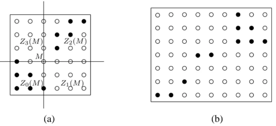
We consider two directions p and q and a point M = hi, ji; it defines the following four zones (called quadrants, see Fig. 1a)):
Z0(hi, ji) = {hi′, j′i ∈ Z2 : i′ ≤ i and j′ ≤ j)},
Z1(hi, ji) = {hi′, j′i ∈ Z2 : i′ ≥ i and j′ ≤ j},
Z2(hi, ji) = {hi′, j′i ∈ Z2 : i′ ≥ i and j′ ≥ j},
Z3(hi, ji) = {hi′, j′i ∈ Z2 : i′ ≤ i and j′ ≥ j}.
Definition 2.1. A lattice set F is Q-convex (quadrant-convex) around D = {p, q} if Zt(M) ∩ F 6= ∅ for all t ∈ {0, 1, 2, 3} implies M ∈ F.
We denote the class of lattice sets which are Q-convex around the directions of D by Q(D). When a lattice set is Q-convex around the specified set of direc-tions, we shortly say that the set is Q-convex. Fig. 1 shows some examples of lattice sets having different kinds of convexity, when the considered directions are p = x and q = y.
(a) (b) M Z3(M ) Z1(M ) Z0(M ) Z2(M )
Fig. 1. a) A lattice set which is line-convex with respect to (1, 0) and (0, 1), but not Q-convex. b) A lattice set Q-convex around (1, 0) and (0, 1).
Definition 2.2. A lattice set F is indivisible for the direction p, or p-indivisible, if {i ∈ Z : |{N ∈ F | p(N) = i}| > 0} is made up of consecutive integers.
By definition, if F is p-indivisible lattice set, then there are i1, i2 ∈ Z such
that the line p = i contains a point of F if and only if i1 ≤ i ≤ i2. If F is
p-and q-indivisible with D = {p, q}, we say that F is D-indivisible or shortly, indivisible. The lattice set shown in Fig. 1a) is indivisible, whereas that in Fig. 1b) is not. An example of an indivisible lattice set which is line-convex with respect to the directions p = x − y and q = x + y, but not Q-convex, is given in Fig. 2. 0 0 3 2 1 2 1 0 1 1 3 1 0 1 1 1 X(1,1)F X(−1,1)F
Fig. 2. An indivisible lattice set which is line-convex with respect to (1, 1)and (−1, 1), but not Q-convex.
In case p = x and q = y, we can establish the following interesting relation-ship between indivisible Q-convex sets and hv-convex 8-connected sets. Proposition 2.3. Let p = x and q = y. An indivisible lattice set F belongs to Q({p, q}) if and only if F is 8-connected and line-convex with respect to directions p and q.
Proof. Let p = x and q = y and let F be an 8-connected and hv-convex set. The set F is 8-connected, so it is indivisible. Suppose that for any i ∈ {0, . . . , 3} we have a point Mi ∈ Zi(M)∩F . We are going to prove that M ∈ F . Consider
first M0 and M1 and let M0 = A0, . . . , Ai, . . . , Ak = M1 the shortest 8-path in
F (it is the path which minimizes k). Since this path is the shortest one and F is hv-convex, the path is monotone, namely, the two sequences (p(Ai)) and
is in the path (see Fig. 3a)). By considering a path from M2 to M3 we can
prove in a similar way that there exists a point N2 ∈ F ∩ (Z2(M) ∩ Z3(M)).
Since the point M is in the vertical segment [N1, N2], M belongs to F .
Conversely, suppose F is an indivisible Q-convex set. F is hv-convex because of the Q-convexity. Let M and N be two points of F and xM < xN and
yM < yN (see Fig. 3b)). We construct an 8-path from M to N. Let M1 =
a)
b)
N
M
1M
3M
2Z
1(M
2)
M
M
2M
0M
N
1M
1M
3Z
3(M
1)
Fig. 3. a) An 8-path from M0 to M1 intersecting Z0(M ) ∩ Z1(M ). b) Constructing
an 8-path from M to N .
(xM, yM + 1), M2 = (xM + 1, yM) and M3 = (xM + 1, yM + 1). Suppose that
none of them belongs to F . Since F is Q-convex, if M1 6∈ F there is at least one
zone Zi(M1) such that Zi(M1)∩F = ∅. We deduce i = 3, because N ∈ Z2(M1)
and M ∈ Z0(M1) ∩ Z1(M1). By proceeding analogously for M2, we deduce
Z1(M2) ∩ F = ∅ and for M3, we have Z1(M3) ∩ F = ∅ or Z3(M3) ∩ F = ∅.
If Z1(M3) ∩ F = ∅, then the line x = xM + 1 does not contain points of F ,
contradicting the hypothesis of indivisibility. If Z3(M3) ∩ F = ∅, then the line
y = yM + 1 does not contain points of F , also contradicting the hypothesis of
indivisibility. Therefore one of the three points M1, M2, M3 belongs to F , say
M1, and (M, M1) constitutes the first step in the construction of any 8-path
from M to N. Continuing in this way, we obtain the searched path.
Let us now introduce the reconstruction problem. Consider any finite subset F of Z2: the X-ray of F in a lattice direction p is the function X
pF : Z → N
defined by: XpF (i) = |{N ∈ F | p(N) = i}|, where i ∈ Z. By definition, XpF
gives the number of points in F on each line parallel to p. Let us define pmin = min{i : XpF (i) > 0}, pmax = max{i : XpF (i) > 0},
qmin = min{j : XqF (j) > 0}, qmax = max{j : XqF (j) > 0},
The set F is finite and so the set of lines intersecting F is also finite. Thus, a vector of nonnegative integers gives a suitable representation for any X-ray of F . The inverse reconstruction problem can be formulated as follows:
Reconstruction2Qconv (Reconstruction of Q-convex sets from X-rays in two directions)
Instance: Two directions p and q and two vectors p = (ppmin, . . . , ppmax),
q= (qqmin, . . . , qqmax) of nonnegative integers.
Task: Reconstruct a set F ∈ Q({p, q}) such that XpF (i) = pi, XqF (j) = qj
for all i ∈ [pmin, pmax] and j ∈ [qmin, qmax], if one exists. 3 Reconstruction algorithm for two directions
In this section we suppose that one instance of Reconstruction2Qconv is given. Without loss of generality we can assume ppmin> 0, ppmax > 0, qqmin >
0, qqmax > 0. Let ∆ denote the parallelogram:
∆ = {M = hi, jip,q ∈ Z2 : pmin ≤ i ≤ pmax, qmin ≤ j ≤ qmax}.
If α and β are two subsets of Z2 we denote the set of all the solutions F
of Reconstruction2Qconv which verify α ⊆ F ⊆ β by E(α, β). The re-construction problem just consists in determining if E(∅, Z2) is empty or not
and in reconstructing a member of it in the latter case. We have trivially E(∅, Z2) = E(∅, ∆). We cannot determine E(∅, ∆) directly, but if E(∅, ∆) 6= ∅
then there exist U1 and U2 ∈ ∆ with p(U1) = pmin and p(U2) = pmax such
that E({U1, U2}, ∆) is not empty.
In the next part, we fix U1, U2 ∈ ∆ such that p(U1) = pmin, p(U2) =
pmax. (These points are called the p-base points). Our aim is to check if E({U1, U2}, ∆) is empty or not. Moreover we suppose that q(U1) ≤ q(U2).
(The case q(U1) ≥ q(U2) is similar.)
3.1 The set H
The first step consists in finding a set H such that E({U1, U2}, ∆) = E({U1, U2}, H).
For this we define the four partial sums: S0(hi, ji) = S0(i) =
X i′≤i pi′ S1(hi, ji) = S1(j) = X j′≤j qj′
S2(hi, ji) = S2(i) =
X i′≥i pi′ S3(hi, ji) = S3(j) = X j′≥j qj′. (3.1)
If S0(pmax) = S2(pmin) =Ppmaxi=pminpiis different from S1(qmax) = S3(qmin) =
Pqmax
j=qminqj, then we know that there cannot be any solution. So we suppose
that these two numbers are equal. Let us define S by:
S = X pmin≤i≤pmax pi = X qmin≤j≤qmax qj. (3.2)
These sums satisfy the following easy but fundamental lemma:
Lemma 3.1. Let M = hi, ji with i, j ∈ Z. If Sk(M) + Sk+1(M) > S, then
F ∩ Zk(M) 6= ∅ for any F ∈ E(∅, ∆), where k + 1 = 0 for k = 3.
Proof. At first we take k = 0 into consideration. If F ∩ Z0(M) = ∅, then
S0(M) + S1(M) = |F ∩ (Z3(M) ∪ Z1(M))| ≤ S. Analogously, cases k = 1, 2, 3
can be proven.
For each line p = i such that pi > 0 we can define two q-indices, as follows:
ai = min{j : S1(j) + S2(i) > S} (3.3)
bi = max{j : S3(j) + S0(i) > S}. (3.4)
Lemma 3.2. If pi > 0, then ai ≤ bi, for i ∈ [pmin, pmax].
Proof. By (3.3) we have that S1(ai − 1) + S2(i) ≤ S. Since S1(ai − 1) =
S − S3(ai) and S2(i) = S − S0(i − 1), the inequality can be rewritten as
S3(ai) + S0(i − 1) ≥ S. If pi > 0, then S0(i − 1) < S0(i) and therefore,
S3(ai) + S0(i) > S. In view of (3.4), this implies ai ≤ bi.
Now we define the sequence ci as follows:
ci = q(U1), if ai < q(U1)
ci = ai, if q(U1) ≤ ai ≤ bi ≤ q(U2)
ci = q(U2), if bi > q(U2)
Lemma 3.3. Let F ∈ E({U1, U2}, ∆} and C = hi, cii ∈ Q2. If pi > 0, then
Zk(C) ∩ F 6= ∅, ∀k ∈ {0, . . . , 3}.
Proof. • If ai < q(U1), we have C = hi, q(U1)i and so U1 ∈ Z0(C) ∩ Z3(C)
and U2 ∈ Z2(C) because of q(U1) < q(U2). Moreover, by the definition of
ai it follows that S1(C) + S2(C) > S and then, by Lemma 3.1, we conclude
Z1(C) ∩ F 6= ∅.
• If q(U1) ≤ ai ≤ bi ≤ q(U2), then C = hi, aii. So, U1 ∈ Z0(C) and U2 ∈
Z2(C). By the definition of ai, S1(C)+S2(C) > S and therefore Z1(C)∩F 6=
∅. Finally, we use the fact that q(C) = ai ≤ bi and S3(C) + S0(C) > S to
conclude that Z3(C) ∩ F 6= ∅.
• If bi > q(U2), then we have C = hi, q(U2)i. It follows that U2 ∈ Z1(C) ∩
Z2(C) and U1 ∈ Z0(C). By the definition of bi, S3(C) + S0(C) > S and so
Z3(C) ∩ F 6= ∅.
Thus, if the point C is in Z2, then it is also in F for any F ∈ E({U
1, U2}, ∆).
ci and hi, ji ∈ Z2} and δ = | det(p, q)|. We have
c′
i ≤ ci ≤ c′i+ δ and hi, c′ii, hi, c′i+ δi ∈ Z2.
Lemma 3.4. LetF ∈ E({U1, U2}, ∆). If pi > 0, then F ∩ {hi, c′ii, hi, c′i+ δi} 6=
∅.
Proof. Let A = hi, c′
ii, B = hi, c′i+ δi, and C = hi, cii. Lemma 3.4 states that
Zk(C) ∩ F 6= ∅, for any k. Since pi > 0, there exists a point N ∈ F such that
p(N) = i.
• If q(N) ≤ q(C), then N ∈ Z0(A)∩Z1(A). We have Z2(C) ⊆ Z2(A), Z3(C) ⊆
Z3(A) and therefore Z2(A) ∩ F 6= ∅, Z3(A) ∩ F 6= ∅. By the Q-convexity of
F we deduce A ∈ F .
• If q(N) ≥ q(C), then N ∈ Z2(B) ∩ Z3(B). Since Z0(C) ⊆ Z0(B), Z1(C) ⊆
Z1(B), by the same arguments as above we can conclude that B ∈ F .
Now let us introduce the following set H:
H = {hi, ji ∈ Z2 : pi > 0, qj > 0, ci− δpi < j ≤ ci + δpi}.
Using this definition we can reformulate the previous lemma as follows: Lemma 3.5. E({U1, U2}, ∆) = E({U1, U2}, H}.
By the definition of H we also have:
Lemma 3.6. In each line p = i there are at most 2pi points of H for all
i ∈ {pmin, . . . , pmax}. 3.2 The filling operations
The previous section shows that E({U1, U2}, Z2) = E({U1, U2}, H). Now we
look for more precise pairs α, β ⊂ Z2 such that E({U
1, U2}, Z2) = E(α, β),
where α is a subset of any F ∈ E({U1, U2}, Z2), whereas β \ α contains
inde-terminate points in the sense that we do not know whether they are in F or not.
So, at the beginning we instantiate α = {U1, U2} and β = H, and then we
expand α and reduce β by means of some operations. All the operations are performed separately on the lines p = i and q = j.
Let us denote the set of points of the intersection between p = i (q = j) and β by βi
p (βqj) and the set of points of the intersection between p = i (q = j)
and α by αi p (αjq). We also define: g(αi p) = min M∈αi p q(M), d(αi p) = max M∈αi p q(M), g(βi p) = min M∈βi p q(M), d(βi p) = max M∈βi p q(M). Here are the four operations ⊕, ⊗, ⊖, ⊙ already described in [3] adapted to
• If αi
p 6= ∅, then ⊕αip = {hi, ji : g(αip) ≤ j ≤ d(αip)}.
• ⊗αi
p = {hi, ji : d(βpi) − δpi < j < g(βpi) + δpi}.
• If αi
p 6= ∅, hi, j′i /∈ βpi with j′ ≤ g(αpi), then ⊖βpi = {hi, ji ∈ βpi : j > j′}.
If αi
p 6= ∅, hi, j′i /∈ βpi with j′ ≥ d(αpi), then ⊖βpi = {hi, ji ∈ βpi : j < j′}.
• If αi
p 6= ∅, then ⊙βpi = {hi, ji ∈ βpi : d(αpi) − δpi < j < g(αip) + δpi}.
To these four operations we add a last operation denoted by ⊙′ which allows
us to delete in β a sequence of consecutive indeterminate points of p = i, when the sequence is shorter than pi.
⊙′βi p =
\
hi,j′i,hi,j′′i∈Z2\β 0<j′′−j′≤δpi
{hi, ji ∈ βi
p : j < j
′ or j > j′′}.
The filling operations on the q-lines are defined analogously.
The algorithm performs all these operations on the p-lines and on the q-lines and repeats this procedure until α 6⊂ β or no further changes in α and β are produced. If we obtain α 6⊂ β, then E({U1, U2}, Z2) = ∅. Therefore, the
algorithm chooses two different p-base points and tries again.
If α = β, then E({U1, U2}, Z2) = E(α, β) ⊆ {α}. So, it only remains to
check if α is Q-convex. Finally, we can obtain the case in which α and β are invariant with respect to the filling operations and α ⊂ β, so that β \ α is not empty.
3.3 The types of lines
Now we suppose that α, β are invariant by the filling operations and verify {U1, U2} ⊆ α ⊂ β ⊆ H.
We will prove in this section that α and β have very particular forms on the p-lines and q-lines.
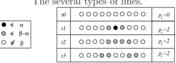
Table 1 shows four types of lines; black, gray and white-colored points rep-resent a point of α, an indeterminate point and a point which does not belong to β, respectively.
Table 1
The several types of lines.
p =0i p =2i p =2i p =2i t3 t1 t0 t2 β−α α β
More precisely, the line p = i is of type: • t0, if βpi = ∅; • t1, if αip 6= ∅; then we have: αi p = {hi, ji : g(α i p) ≤ j ≤ d(α i p)}
βi
p = {hi, ji : g(αip) − δ(pi− |αip|) ≤ j ≤ d(αip) + δ(pi− |αip|)};
• t2, if αip = ∅ and βpi is made up of 2pi consecutive points. So we have
βpi = {hi, ji : g(β i
p) ≤ j < g(β i
p) + 2δpi};
• t3, if αip = ∅ and βpi consists of two separated sequences of pi points. So:
βpi = {hi, ji : g(β i p) ≤ j ≤ g(β i p)+δ(pi−1) or d(βpi)−δ(pi−1) ≤ j ≤ d(βpi)} with d(β i p)−g(β i p) ≥ 2p
Since we know that β ⊆ H, thanks to Lemma 3.6 we can claim that:
Proposition 3.7. After performing the filling operations, each line having equation p = i is of type t0, t1 or t2, i ∈ [pmin, pmax].
Let p = i be any p-line. From Proposition 3.7, we deduce that: |βi
p| = 2pi− |αip| for all i ∈ [pmin, pmax].
By summing over i we have
|β| = 2S − |α|. (3.5)
Consider now the q-lines and let q = j be the equation of any line containing indeterminate points. Thanks to the operations ⊗ and ⊙′, we have:
|βj q| ≥ 2qj− |αjq| and therefore, |β| =X j |βj q| ≥ X j (2qj− |αjq|) = 2S − |α|. By (3.5) we deduce: |βj
q| = 2qj− |αjq| for all j ∈ [qmin, qmax];
otherwise we get a contradiction. We note that this result allows us to deter-mine the type of the q-lines. In fact, when |αj
q| > 0 we know that q = j is a
line of type t1. If |αjq| = 0 then we have |βqj| = 2qj; thanks to the operation
⊙′ this means that the set βj
q is made up of two sequences having the same
length, being either consecutive (in this case q = j of type t2) or separate (in
this case q = j of type t3).
Proposition 3.8. After performing the filling operations, each line having equation q = j is of type t0, t1, t2 or t3, j ∈ [qmin, qmax].
3.4 Reduction to a 2-SAT formula
For each point M ∈ ∆\α we associate a boolean variable VM expressing the
Each instantiation of the boolean variables VM gives a set α ⊆ F (V ) ⊆ β
where
F (V ) = α ∪ {M ∈ β \ α : VM = T RUE}.
Now we construct a boolean formula whose variables are (VM)M∈β\αin such
a way that F (V ) is a Q-convex set having the given X-rays. Therefore the reconstruction problem will be reduced to the search of a truth assignment of the variables for the formula. Since this formula is a 2-SAT formula, its satisfiability can be easily checked (see [1]).
3.4.1 Expression ofXqF (j) = qj
We fix a line q = j. This line is of type ti with i ∈ {0, . . . , 3} and so, there
are exactly 2(qj−|αip|) unknown points on each line q = j. If the line is of type
t1 or t2, and A = hi, ji, B = hi + δpi, ji ∈ β \ α, then for any set F ∈ E(α, β)
we have
A ∈ F if and only if B /∈ F so we can express XqF (j) = qj by the formula:
F Qj =
^
hi,ji,hi′,ji∈β\α i′−i=δqj
Vhi,ji⇐⇒ Vhi′,ji.
If the line is of type t3, then this line is made up of two sequences of
consecu-tive indeterminate points. Since we know that each set F ∈ E(α, β) contains exactly one of these sequences, in this case we can express XqF (j) = qj by
the formula: F Qj = ^ hi,ji,hi′,ji∈β\α i′−i>δqj Vhi,ji⇐⇒ Vhi′,ji.
In the same way we can express that XpF (i) = pi by a similar formula F Pi.
3.4.2 Expression of the Q-convexity
Now we impose that the set F (V ) is Q-convex. We can find a direct boolean formula which expresses that for any M /∈ F (V ) there is a quadrant Zi(M)
containing no points of F (V ) but this formula is a disjunction of 5 variables or negations of variables, that is not a 2-SAT formula.
Remark 3.9. Let M = hi, jip,q be a point of Z2\ α which verifies one of the
following properties:
• q(M) = j (resp., p(M) = i) is a t1 q-line (resp., p-line) or a t2 q-line (resp.,
p-line).
• q(M) = j is a t3 q-line such that d(βqj)−δ(qj−1) ≤ i or i ≤ g(βqj)+δ(qj−1).
Then, one of the two semi-lines Λ−
q(M) = {hi′, ji : i′ ≤ i} and Λ+q(M) =
{hi′, ji : i′ ≥ i} (resp., Λ−
p(M) = {hi, j′i : j′ ≤ j} and Λ+p(M) = {hi, j′i :
j′ ≥ j}) contains a point of F for any F ∈ E(α, β). We denote this semi-line
• if the line is of type t1, then Λq(M) is the semi-line containing a point of
αj q;
• if the line is of type t2 or t3 and M /∈ β, then Λq(M) is the semi-line
containing all the points of βj q;
• if the line is of type t2 or t3 and M ∈ β, then we have Λ−q(M) ∩ Λ+q(M) =
{M} ⊆ βj
q and |βqj| = 2qj. So, one of the semi-lines verifies |Λ·q(M)∩βqj| > qj.
This semi-line contains at least one point of any F ∈ E(α, β). Let g′(βj
q) = g(βqj) + δ(qj− 1) and d′(βqj) = d(βqj) − δ(qj − 1); as a summary,
if g′(βj
q) ≥ i, then Λq(M) = Λ+q(M), whereas if d′(βqj) ≤ i, then Λq(M) =
Λ− q(M).
Now we will express the Q-convexity of F (V ) around M ∈ ∆ \ α by means of a 2-SAT boolean formula.
• At first, suppose that p(M) = i and q(M) = j verify Remark 3.9. Thanks to the semi-lines Λp(M) and Λq(M) we can find an integer k ∈ {0, . . . , 3}
such that for any l 6= k and any F ∈ E(α, β) we have Zl(M) ∩ F 6= ∅.
· If M /∈ β and Zk(M) ∩ α 6= ∅, then we have E(α, β) = ∅, so we can express
the Q-convexity by the formula
F ALSE. (3.6)
· If M /∈ β and Zk(M) ∩ α = ∅, the formula is:
VN (3.7)
for any N ∈ Zk(M) ∩ β.
· If M ∈ β and Zk(M) ∩ α 6= ∅, the formula is:
VM. (3.8)
· If M ∈ β and Zk(M) ∩ α = ∅, the formula is:
VN ⇒ VM (3.9)
for any N ∈ Zk(M) ∩ β.
• Suppose now that M /∈ β, and at least one of the lines p(M) = i and q(M) = j does not verify the conditions in Remark 3.9. Since we know that U1, U2 ∈ α, there are at most two quadrants which do not contain any
point of α. If there is no or only one such quadrant, then we can express the Q-convexity by formulas (3.6) and (3.7). Otherwise there are exactly two quadrants Zl1(M) and Zl2(M) which do not contain any point of α.
- If p = i is a t0-line, or q = j is a t0-line or a t3-line such that g(βqj) + δqj ≤
i ≤ d(βj
q) − δqj, then we can express the Q-convexity around M by the
formula:
VN1 ∨ VN2 (3.10)
Now we briefly summarize the reconstruction procedure, describing its main steps and their complexities. The analysis of the computational cost of every step is given in the appendix.
The algorithm checks whether the given X-rays satisfy the necessary condition on the cumulated sums to get a solution, and then it fixes two p-base points or two q-base points depending on the sizes of the X-ray vector. (If m < n, the p-base points are chosen). The cost of this choice is min{m2, n2}, the number of
possible positions of the base points. Furthermore let us assume that the p-base points U1 and U2are chosen. At this point, since E(∅, ∆) ⊇ E({U1, U2}, ∆), the
problem is reduced to checking if E({U1, U2}, ∆) is empty or not. To this goal,
the algorithm works to reduce the set containing the solution by computing the set H (only depending on the X-rays and p-base points). This is made in O(mn) time. Then, sets α and β are initialized and the filling operations are performed to expand α and reduce β in such a way that the following property is preserved: E({U1, U2}, H) = E(α, β). The computational cost of this step
is O(mn(m + n)). Finally, the algorithm builds a boolean formula such that each assignment of values of the variables satisfying the formula gives rise to a solution F (V ) of our reconstruction problem. Since both the construction and the satisfiability of the formula take O(mn(m + n)) time, one knows if E(α, β) is empty or not in O(mn(m + n)) time.
Proposition 3.10. Reconstruction2Qconvis solvable inO(min{m2, n2}(mn(m+
n))) time.
Remark 3.11. From the previous remark and Lemma 2.3 it follows that our algorithm solves the problem of reconstructing 8-connected hv-convex sets from its X-rays in directions p = x, q = y in polynomial time.
4 More than two X-rays
In this section, we study the general problem with more than two X-rays. Now the question is the following: is it possible to reconstruct a Q-convex set from its X-rays taken in a prescribed set of d directions? Let us concentrate on the case d = 3. Let D be a set of three lattice directions p = λpx + µpy, q =
λqx+ µqy, r = λrx+ µry. Moreover we assume det(p, r) = λpµr−µpλr 6= 0 and
det(q, r) = λqµr− µqλr 6= 0. Now a point M of Z2 is the intersection of three
lines having equations p(M) = i, q(M) = j and r(M) = k and it determines three kinds of quadrants Ztpq(M), Z
qr
t (M) and Z rp
t (M), for t = 0, 1, 2, 3 related
to the pairs of directions {p, q}, {q, r} and {r, p}, respectively.
Definition 4.1. A lattice set F is Q-convex around {p, q, r} if it is Q-convex around {p, q}, {q, r} and {r, p}. More generally, a lattice set is Q-convex around a set D of directions if it is Q-convex around any pair of direction included in D.
Proposition 4.2. Let p = x, q = y and r = x − y be the horizontal, vertical and diagonal directions. An indivisible lattice set F belongs to Q(D) if and
only if F is 6-connected and line-convex with respect to the directions q, p and r.
Proof. If F is 6-connected, it is also 8-connected and therefore F is indivisible and Q-convex around {p, q}. Since there exists an isomorphism of Z2 which
transforms r-lines into q-lines but leaves p-lines invariant, we can conclude that F is indivisible and Q-convex around {p, r}. Analogously, the isomorphism of Z2 which transforms r-lines into p-lines, leaving q-lines invariant, allows us to say that F is indivisible and Q-convex around {q, r}.
Conversely, suppose that F is an indivisible Q-convex set; we show that for each pair (M, N) of F points there is 6-path from M = (xM, yM) to N =
(xN, yN) in F . Let N be such that xM < xN, yM < yN and yN ≤ xN (the
other cases can be proven by symmetry). Moreover, let M1 = (xM+ 1, yM+ 1)
and M2 = (xM + 1, yM). By the indivisibility of F , there is a point M′ of F
on the line x = xM + 1. If yM′ ≤ yM2 (see Fig. 4a)), by the Q-convexity of F
around {p, q}, M2belongs to F so that the first step of the path is determined.
So, let us suppose yM′ > yM2 (see Fig. 4b)); by the Q-convexity of F around
{p, r} M1 belongs to F so that the first step of the path is determined.
(a) (b) M2 M M1 N M2 M M1 N M′ M′ Fig. 4. a) yM′ ≤ yM2. b) yM′ > yM2.
Our algorithm can be easily extended in order to work for a set D = {p, q, r} of three directions for reconstructing lattice sets which are Q-convex around D. First the algorithm chooses the p-base-points U1, U2; then it constructs the
set H just considering the pairs p, q of directions and after that it performs the filling operations in all the given directions. In this way, the set of all the solutions is more accurately specified at each step:
E({U1, U2}, ∆) = E({U1, U2}, H) = E(α, β).
It is easy to see that in this case too, all the p-lines, q-lines, r-lines are of type ti, i ∈ {0, . . . , 3}. All the formulas expressing that F (V ) is a solution
because in expressing the Q-convexity in M around q, r the two points U1 and
U2 can be in the same quadrant.
To study this case, we generalize Remark 3.9 to points of Q2.
Remark 4.3. Let M = hj, kiq,r be a point of Q2\ α which verifies one of the
following properties: (M can be in Q2 \ Z2.)
• q(M) = j is a t1 q-line.
• q(M) = j is a t2 or t3 q-line and d′(βqj) ≤ k or k ≤ g′(βqj).
Then, one the two semi-lines Λ−
q(M) = {hj, k′iq,r : k′ ≤ k} and Λ+q(M) =
{hj, k′i
q,r : k′ ≥ k} contains a point of F for any F ∈ E(α, β). More precisely,
if g′(βj
q) ≥ k, then Λq(M) = Λ+q(M), whereas if d′(βqj) ≤ k, then Λq(M) =
Λ− q(M).
Suppose that M = hj, kiq,r is a point of ∆ \ β not verifying the conditions of
Remark 3.9 on the lines q(M) = j and r(M) = k. Moreover, U1 and U2 are in
the same quadrant, for example Z0qr(M). If there exists a point N such that r(N) = r(M) and q(N) ≥ q(M) verifying the conditions of Remark 4.3, then we know that Zhqr(M) ∩ F 6= ∅ with h ∈ {1, 2} for any F ∈ E(α, β) and this
case is analogous to one of the two-directions cases. Therefore, we can suppose that q(M) = j and r(M) = k are t0 or t3 lines and all the lines q = j′ with
j′ ≥ j are of type t
0 and, t2 or t3 such that g′(βj ′
q ) < k < d′(βj ′
q). The same
assumption is made for all the lines r = k′ with k′ ≥ k. As a consequence of
formulas F Q and F R, each indeterminate point N ∈ Z2qr(M) is associated to
a point N′ ∈ Zqr
1 (M) and to a point N′′ ∈ Z qr
3 (M), by the formulas
VN ≡ VN′ ≡ VN′′. (4.11)
Therefore, we can express the Q-convexity in M as:
VN1 ⇔ VN2 (4.12)
for any N1, N2 ∈ (β \ α) ∩ Z2qr(M). The algorithm constructs the boolean
formula and checks its satisfiability in O(n3) time where n = max(pmax −
pmin, qmax − qmin, rmax − rmin). Since performing the filling operations takes O(n3) and the number of attempts is bound by n2 (=number of possible
choices for U1 and U2), the complexity of this algorithm is O(n5).
Remark 4.4. From Lemma 4.2 it follows that our algorithm solves the prob-lem of reconstructing 6-connected hvd-convex sets from their X-rays in direc-tions p = x, q = y, r = x − y in polynomial time.
We can generalize the algorithm in order to work with any number d of directions. The precise problem we solve is the following:
ReconstructionQconv
Instance:A set of directions D = {v1, . . . , vd} and d vectors (pvi(minvi), . . . , pvi(maxvi))1≤i≤d.
Task:Reconstruct a set F ∈ Q(D) such that XviF (j) = pvi(j) for all i ∈ [1, d]
In this case the Q-convexity is expressed for all the pairs (vi, vj) such that
1 ≤ i < j ≤ d, so we can construct a solution in O(d2n5), where n is the
maximal length of the X-rays (n = max(maxvi− minvi)).
Proposition 4.5. ReconstructionQconv is solvable in O(d2n5) time.
This generalization is particularly interesting in view of a new result of Daurat [8,7] establishing when subsets of Q(D) are uniquely determined by the data: Theorem 4.6. If |D| ≥ 7, or if one of the cross-ratios of the slopes of any four directions, arranged in increasing order, is not in {4
3, 3
2, 2, 3, 4} then for
any sets E, F ∈ Q(D) we have:
∀p ∈ D XpE = XpF =⇒ E = F.
In this paper we establish the complexity of the related algorithmic prob-lem, showing that the reconstruction problem in Q(D) is solvable in polyno-mial time. Let us stress that the class of Q-convex sets contains the class of sets that are equal to the intersection of their convex hull and Z2, namely, the
class of convex sets. Thus, the most important application of the proposed algorithm is that it allows to reconstruct a convex lattice set from its X-rays taken in any certain set of directions, so answering the question proposed by Gritzmann during the workshop held in Dagstuhl in 1997. Precisely let us define the following problem:
ReconstructionConv
Instance: A set of directions D = {v1, . . . , vd} such that d ≥ 7 or one of the
cross-ratios of the slopes of four directions, arranged in increasing order is not in {43,32, 2, 3, 4} and d vectors (pvi(minvi), . . . , pvi(maxvi))1≤i≤d.
Task: Reconstruct a convex set such that XviF (j) = pvi(j) for all i ∈ [1, d]
and j ∈ [minvi, maxvi].
Theorem 4.7. ReconstructionConv can be solved in O(d2n5) time.
Proof. Let (D, (pvi)1≤i≤|D|) be an instance of ReconstructionConv. By the
algorithm of Proposition 4.5, we can check if there is a Q-convex set around D which has X-rays (pvi). If there is no Q-convex solution, then a fortiori there
is no convex solution. Otherwise we have found the Q-convex set F whose X-rays are (pvi). By Theorem 4.6 the set F is in fact the unique Q-convex set
having (pvi) as X-rays. So, we only have to check if F is convex. This check
can be done by computing the convex hull of F in R2 (see for example [12])
and then filling the convex polygon to check that F = conv(F ) ∩ Z2.
Remark 4.8. After the submission of this paper, the authors and A. Del Lungo have found an algorithm designed for approximate reconstruction prob-lems. It has already been published in [5]. The class of lattice sets studied in [5] is obtained by extending the definition 2.1 in a different way than 4.1. The resulting class, so-called strongly Q-convex, is a subclass of that of Q-convex sets. The algorithm proposed in [5] also permits to reconstruct the convex sets
as a special case, but it is much slower since d (number of directions) appears at the exponent of n.
5 Some considerations and conclusions
The most significant result of this paper is a polynomial-time algorithm for the reconstruction of uniquely determined convex lattice sets. But this result leads to two questions:
Can we decrease the complexity of our algorithm ? This question is impor-tant because the complexity of our algorithm can look still high for real appli-cations. At a closer look, the number of possible choices for U1 and U2 causes
the growth of the exponent of n from 3 to 5. Thus, in a smarter implementation of the algorithm, at first no base-points are chosen but the filling operations are performed; then, one base-point is fixed, and finally, only if necessary to reach the solution after failing the previous attempts, two base-points are selected. This variant probably improves the average case. Preliminary exper-iments ([8]) indicate an estimated average case complexity of O(n2.8) because
in most cases the bases need not to be chosen a priori, but much work should be done, and in particular we need an algorithm which generates uniformly convex lattice sets of a given size at random.
Secondly what can we say about the reconstruction problem for any set of lattice directions not uniquely determining convex lattice sets ? Does there exist a polynomial algorithm in this case ? We could apply our algorithm until the reduction to a 2-SAT formula, but then we do not see any way to express the convexity by a formula whose satisfiability could be checked in polynomial time.
6 Appendix
In this section we analyze the computational cost of computing the main steps of the reconstruction algorithm.
6.1 Performing the filling operations
In implementing the filling operations we use 5 supplementary variables for each p-line and each q-line. Consider the line p = i; we denote theses variables by toput⊕i
p, toput⊗ip, toremove⊖ip, toremove⊙ip, toremove⊙′ip
con-taining the points to be modified if we would apply the corresponding fill-ing operations. Algorithm 1 describes the procedure performfill-ing the fillfill-ing operations. Let us now compute the time-complexity of this algorithm. The procedure compute points to change needs O(m + n) operations. It follows that put in alpha and remove from beta have also a complexity of O(m + n). In the main procedure executing the repeat loop (lines 8-18) takes O(m +
Algorithm 1Implementation of the filling operations compute points to change(p, i)
1: for all ⊘ ∈ {⊕, ⊗} do 2: toput⊘i p ← ⊘(αip) \ αip 3: end for 4: for all ⊘ ∈ {⊖, ⊙, ⊙′} do 5: toremove⊘i p ← βpi \ ⊘(βpi) 6: end for put in alpha(M) 1: if M /∈ β then 2: EXIT(no solution) 3: end if 4: α ← α ∪ {M}
5: compute points to change(p, p(M))
6: compute points to change(q, q(M)) remove from beta(M)
1: if M ∈ α then
2: EXIT(no solution)
3: end if
4: β ← β \ {M}
5: compute points to change(p, p(M))
6: compute points to change(q, q(M)) main()
1: for all i ∈ {pmin, . . . , pmax} do
2: compute points to change(p, i)
3: end for
4: for all j ∈ {qmin, . . . , qmax} do
5: compute points to change(q, j)
6: end for
7: repeat
8: for all i ∈ {pmin, . . . , pmax} do
9: for all ⊘ ∈ {⊕, ⊗} and M ∈ toput⊘i p do
10: put in alpha(M)
11: end for
12: for all ⊘ ∈ {⊖, ⊙, ⊙′} and M ∈ toremove⊘i p do
13: remove from beta(M)
14: end for
15: end for
16: for all j ∈ {qmin, . . . , qmax} do
17: Idem by replacing p by q
18: end for
n + ki(m + n)) operations, where ki is the number of the calls of the
proce-dures put in alpha and remove from beta at the ith iteration. Each time that put in alpha or remove from beta are called, |β \ α| decreases except when an EXIT call is made. Therefore, k1+ k2+ . . . + kr ≤ mn + 1. Moreover we have
that the number of repeat loop iterations is bounded by mn. Therefore the final complexity of the algorithm 1 is O(mn(m + n)).
6.2 Constructing and satisfying the boolean formula 6.2.1 Two directions
In this part we prove that we can build a 2-SAT formula expressing the existence of a solution F ∈ E(α, β) in O((m + n)mn) time.
The formulas F P and F Q. The formulas F Pi, F Qj associated to t1 and
t2 lines can be trivially found in O(mn(m + n)) time. If q = j is of type t3,
constructing the formula F Qj takes O(mn) time, since F Qj is equivalent to
the formula: Vhg(βj
q),ji ⇐⇒ Vhg(βqj)+δ,ji⇐⇒ . . . ⇐⇒ Vhg(βqj)+(qj−1)δ,ji
⇐⇒ Vhd(βj
q)−(qj−1)δ,ji⇐⇒ . . . ⇐⇒ Vhd(βqj),ji
Therefore, all the formulas F Pi, F Qj can be found in O(mn(m + n)) time.
Let us now search the formulas which express the Q-convexity. At first we suppose that we have precomputed the function g, d, g′, d′ for any p-line or
q-line. This computation takes O(mn) operations So now, we can suppose that the time-complexity is constant.
The formulas associated to the points M which verify the remark 3.9. We build formulas (3.6),(3.7),(3.8),(3.9) line by line. Let us consider any line q = j; we show that the formulas associated to the points M of this line can be found in O(mn) time.
We look for the minimum and maximum p-indices such that Λp(M) = Λ−p(M)
and for the minimum and maximum p-indices such that Λp(M) = Λ+p(M).
Formally, we define
i1 = min{i : d′(βpi) ≤ j}, i2 = max{i : d′(βpi) ≤ j},
i′1 = min{i : g′(βpi) ≥ j}, i′2 = max{i : g′(β i
p) ≥ j}.
Thus, the points M ∈ ∆ \ α of q = j under the hypothesis of the remark 3.9 verify:
p(M) ∈ ([i1, i2] ∪ [i′1, i′2]) ∩ ([pmin, g′(βqj)] ∪ [d′(βqj), pmax]).
For instance, we look for all the clauses corresponding to the points M such that p(M) ∈ [i1, i2]∩[pmin, g′(βqj)]. (The other cases are similar). Since p(M) ∈
[i1, i2], Zl(M) ∩ F 6= ∅, l = 0, 1, while by p(M) ∈ [pmin, g′(βqj)] it follows that
Z2(M) ∩ F 6= ∅, for any F ∈ E(α, β). If Z3(M) ∩ α 6= ∅, clauses (3.6),(3.8) can
be easily found in O(mn) time. Clauses (3.7) can be found in O(mn) time, since we construct VN for any N ∈ Z3(M), where M 6∈ β is the point of q = j
maximizing p such that p(M) ∈ [i1, i2] ∩ [pmin, g′(βqj)].
Now we build formulas (3.9). At first we express the line-convexity along the line q = j by the formula:
Vhg(βj
q),ji ⇒ Vhg(βjq)+δ,ji⇒ . . . ⇒ Vhg(βqj)+δ(qj−1−|αjq|),ji. (6.13)
Let lmin, lmax defined by:
{l : hg(βj q)+δl, ji ∈ β\α and g(β j q)+δl ∈ [i1, i2]∩[pmin, g ′(βj q)]} = {lmin, . . . , lmax}.
Then we construct the additional clauses
VNl ⇒ Vhg(βjq)+lδ,ji (6.14)
for all Nl ∈ Z3(hg(βqj) + lδ, ji) if l = lmin and for all Nl∈ Z3(hg(βqj) + lδ, ji) \
Z3(hg(βqj)+(l−1)δ, ji) if l ∈ {lmin+1, . . . , lmax}. It is easy to see that formulas
(6.13) and (6.14) are equivalent to formulas (3.9) associated to all the points M on the line q = j. When the q-line is fixed, all these formulas can be found in O(mn) time. Since there are n q-lines, the global construction takes O(mn2)
time.
The formulas associated to the other points Now we show that also clauses (3.10) can be found in O((mn(m + n)) time. These formulas are built for the points not in β lying on a t0 p-line or on a t0, t3 q-line. Since there
are n q-lines (resp., m p-lines), if for each q-line (resp., p-line) we find these formulas in O(mn + m2)-time (resp., O(mn + n2)), then the construction will
take O(mn(m + n)) time.
The points M that are on a t0-q-line q = j. Three cases should be
considered:
j < q(U1), q(U1) < j < q(U2), q(U2) < j.
Let us examine the case: q(U1) < j < q(U2). Let us define
i1 = max{i : d′(βpi) ≤ j}, i2 = min{i : g ′(βi
the maximum and minimum p-index such that Λp(hi1, ji) = Λ−p(hi1, ji) and
Λp(hi2, ji) = Λ+p(hi2, ji). Thus, Z1(hi1, jip,q) ∩ F 6= ∅ and Z3(hi2, jip,q) ∩ F 6= ∅
for any F ∈ E(α, β). Since hi1, jip,q may not be in Z2, let i′1 = max(i : i ≤
i1, hi, jip,q ∈ Z2). So, we impose the formula VN for any N ∈ Z3(hi′1, jip,q).
Analogously, let i′
2 = min(i : i ≥ i2, hi, jip,q ∈ Z2): we impose VN for any
N ∈ Z1(hi′2, jip,q). Moreover, in each line p = i such that i1 < i < i2 and
pi > 0 we select two special points Ai, Bi ∈ β \ α defined by:
q(Ai) = max
h<j {h : hi, hip,q∈ β \ α}, q(Bi) = minj<h{h : hi, hip,q∈ β \ α}.
To express the Q-convexity around the points of q = j we impose the following clauses:
VAi ⇒ Vhi,q(Ai)−δi⇒ Vhi,q(Ai)−2δi ⇒ . . . ⇒ Vhi,g(βp)ii , (6.15)
VBi ⇒ Vhi,q(Bi)+δi⇒ Vhi,q(Bi)+2δi ⇒ . . . ⇒ Vhi,d(βi
p)i, (6.16)
So, less than mn clauses are constructed. To these ones we should also add the clauses
VAh1 ∨ VBh2, (6.17)
for all pairs (h1, h2) with h2 ≤ i ≤ h1 such that hi, jip,q∈ Z2 and i′1+ δ ≤ i ≤
i′
2− δ. The pairs (h1, h2) can be found in O(m2)-time by the algorithm 2.
Algorithm 2 Enumeration of the pairs (h1, h2) with a ≤ h2 ≤ h1 ≤ b when
there exists i = a + δi′ with i′ ∈ Z, h
2 ≤ i ≤ h1. The complexity of this
algorithm is O((b − a)2) h1 ← a i ← a while h1 ≤ b do while h1 < i + δ do h2 ← a while h2 ≤ i do PRINT (h1, h2) h2 ← h2+ 1 end while h1 ← h1+ 1 end while i ← i + δ end while
It is easy to check that if N1 ∈ Z1(M) and N2 ∈ Z3(M) the constructed
clauses are equivalent to VN1 ∨ VN2. Since we can build clauses (6.15) and
(6.16) in O(n) time and clauses (6.17) in O(m2) time, constructing clauses (3.10) takes O(mn(m + n)) time in case q(U1) < j < q(U2).
Now let us take case j < q(U1) into consideration. If {i : d′(βpi) ≤ j}
is not empty, let i1 and i2 be the minimum and maximum element of the
set, respectively and again i′
min{i : i ≥ i1, hi, jip,q∈ Z2}. If i′1 ≥ i′2, then there is no solution in E(α, β);
otherwise i′
2 = i′1+ δ and so the formulas VN, for any N ∈ Z0(hi′1, jip,q) and
N ∈ Z1(hi′2, jip,q) are imposed. If {i : d′(βpi) ≤ j} is empty, then on each
line p = i such that pi > 0 we select the point Ai such that q(Ai) = max{h :
hi, hip,q ∈ β \ α and 1 ≤ h < j}.
Therefore, the Q-convexity around the points of q = j is expressed by VAi ⇒ Vhi,q(Ai)−δi⇒ Vhi,q(Ai)−2δi ⇒ . . . ⇒ Vhi,g(βi
p)i,
and
VAh1 ∨ VAh2,
for all h2 ≤ i ≤ h1 such that hi, jip,q ∈ Z2 with pmin ≤ i ≤ pmax. Since less
than mn+m2clauses are built, constructing clauses (3.10) takes O(mn(m+n))
time in case j < q(U1).
Case q(U2) > j can be similarly treated being the symmetric case.
The points M that are on a t0-p-line p = i. This case is very similar
to the previous one. As in the previous case we define: j1 = min{j : d′(βqj) ≤ i}, j2 = max{j : d
′(βj q) ≤ i}
j1′ = min{j : g′(βqj) ≥ i}, j2′ = max{j : g′(βqj) ≥ i}.
It follows that j1 ≤ q(U1) ≤ j2 and j1′ ≤ q(U2) ≤ j2′, and moreover j1 ≤ j2′ by
q(U1) ≤ q(U2).
The Q-convexity around the points hi, ji which verify j1 ≤ j ≤ j2 or j1′ ≤
j ≤ j′
2 are expressed by the clauses (3.7).
The Q-convexity around the points hi, ji such that j ≤ min(j1, j1′) or
j2 ≤ j ≤ j1′ or j ≥ max(j2, j2′) can be expressed by similar formulas to
(6.15),(6.16),(6.17) in O(mn + n2)-time.
The points M that are on a t3-q-line q = j. We should express the
Q-convexity in all the points hi, ji such that g(βj
q) + δqj ≤ i ≤ d(βqj) − δqj. Let
N be an arbitrary indeterminate point such that q(N) = j and q(N) ≤ g′(βj q).
Since for each N′, N′′∈ βj
q \ α with p(N′) ≤ g′(βqj) < d′(βqj) ≤ p(N′′) we have
the formula VN ≡ VN′ ≡ VN′′ as a consequence of F Qj, we can express the
Q-convexity by the clauses
(VN ⇒ VN2), (VN ⇒ VN1) (6.18) for each N1 ∈ Zl1(hd(β q j) − δqj, ji) ∩ β and N2 ∈ Zl2(hg(β q j) + δqj, ji) ∩ β where (l1, l2) = (0, 1) if j ≤ q(U1) = (3, 1) if q(U1) ≤ j ≤ q(U2) = (3, 2) if j ≥ q(U2).
These clauses can be found in O(mn) time for each line q = j. 6.2.2 More than two directions
The expression of the Q-convexity in the points M which verify the Remark 3.9 can be computed exactly like in the case of two directions. Here we studied in details the additional cases that need to be taken into account. So, let us consider a line q = j of type t0or t3. We should impose the Q-convexity around
the two directions (q, r) in any point M = hj, kiq,r of ∆ \ β not verifying the
conditions of Remark 3.9. Moreover we suppose q(U1) ≤ j and that U1 and U2
are in the same quadrant Zlqr with l ∈ {0, . . . , 3}. From a brutal computation,
it may seem that the cost of the construction of the formulas (4.12) is O(n4),
so changing the performance of the reconstruction algorithm considerably. Actually, we show that it takes O(n3). We determine the gaps where the
r-indices of the points in q = j need to be considered. Let k1 = min h≥j(d ′(βh q)), k2 = max h≥j(g ′(βh q)) and k1′ = min{k : g′(βrk) ≥ j or d′(β k r) ≤ j)}, k2′ = max{k : g′(β k r) ≥ j or d′(β k r) ≤ j}.
The minima and maxima are taken only over lines intersecting β. The case in which all lines are t0-lines is trivial. Since the line r = r(U1) is a t1-line, by
definitions of k′
1, k2′ the inequality k′1 < r(U1) < k2′ follows.
We express the Q-convexity in all the points M = hj, kiqr of the q-line q = j.
• If k ≥ k1, then ∃h > j Λq(hh, kiq,r) = Λ−q(hh, kiq,r). We know that F ∩
Z1qr(hj, k1iq,r) 6= ∅ for any F ∈ E(α, β). So we can express the Q-convexity
by the formulas (3.10), which can be built by the method which is used for two directions.
• The case k ≤ k2 is similar to the previous one (∃h > j Λq(hh, kiq,r) =
Λ+
q(hh, kiq,r)).
• If k ∈ [k′
1, k′2], then we know that there exist l1 ∈ {0, 1}, l2 ∈ {2, 3} such
that Zlqr1(hj, k ′ 1i) ∩ F 6= ∅ and Z qr l2(hj, k ′
2i) ∩ F 6= ∅ for any F ∈ E(α, β). So,
we can also express the Q-convexity by the formulas (3.10).
• It remains the case k ∈]k2, k1[ \ [k′1, k2′]. If ]k2, k1[∩] − ∞, k′1[6= ∅, define:
k3 = max{k < min(k1′, k2) : hj, kiq,r ∈ Z2}. The Q-convexity in all the
points hj, ki with k ∈]k2, k1[∩] − ∞, k′1[ can be expressed by the formula:
VM1 ⇔ . . . ⇔ VMl
where M1, . . . Ml are the indeterminate points of Z1qr(hj, k3iq,r).
In the same way if ]k2, k1[∩]k2′, +∞[6= ∅ we define: k4 = min{k > max(k1, k′2) :
hj, kiq,r ∈ Z2}. The Q-convexity in all the points hj, ki with k ∈]k2, k1[∩]k′2, +∞[
can be expressed by the formula:
where M1, . . . Ml are the indeterminate points of Z2qr(hj, k4iq,r).
Therefore, the construction of the formulas can be done in O(n2) time, for
each fixed line. In conclusion, since there are at most 2n q-lines and r-lines the clauses to express the Q-convexity can be found in O(n3) time.
References
[1] B. Aspvall, M. Plass, R. Tarjan, A linear-time algorithm for testing the truth of certain quantified boolean formulas, Inform. Process. Lett. 8 (3) (1979) 121–123. [2] E. Barcucci, S. Brunetti, A. Del Lungo, M. Nivat, Reconstruction of discrete sets from three or more X-rays, Proc. of CIAC 2000, Lecture Notes in Comput. Sci., 1767 (2000) 199–210.
[3] E. Barcucci, A. D. Lungo, M. Nivat, R. Pinzani, Reconstructing convex polyominoes from horizontal and vertical projections, Theoret. Comput. Sci. 155 (2) (1996) 321–347.
[4] E. Barcucci, A. Del Lungo, M. Nivat, R. Pinzani, Medians of polyominoes: a property for the reconstruction, Int. J. Imaging Systems and Technol. 8 (1998) 69–77.
[5] S. Brunetti, A. Daurat, A. Del Lungo, Approximate X-rays reconstruction of special lattice sets, Pure Math. Appl. 11 (3) (2000) 409–425.
[6] M. Chrobak, C. D¨urr, Reconstructing HV-convex polyominoes from orthogonal
projections, Inform. Process. Lett. 69 (6) (1999) 283–289.
[7] A. Daurat, Uniqueness of the reconstruction of Q-convexes from their projections., preprint LLAIC1 (2000).
[8] A. Daurat, Convexit´e dans le plan discret, application `a la tomographie discr`ete,
Ph.D. thesis, LLAIC1 and LIAFA, Universit´e Paris 7 (2000).
[9] A. Daurat, A. Del Lungo, M. Nivat, Median points of discrete sets according to a linear distance, Discrete Comput. Geom. 23 (2000) 465–483.
[10] R. J. Gardner, P. Gritzmann, D. Prangenberg, On the computational complexity of reconstructing lattice sets from their X-rays, Discrete Math. 202 (1999) 45–71.
[11] R. J. Gardner, P. Gritzmann, Discrete tomography: Determination of finite sets by X-rays., Trans. Amer. Math. Soc. 349 (6) (1997) 2271–2295.
[12] R. L. Graham, An efficient algorithm for determining the convex hull of a finite planar set, Inform. Process. Lett. 1 (4) (1972) 132–133.
[13] G. H. Woeginger, The reconstruction of polyominoes from horizontal and vertical projections, Inform. Process. Lett. 77 (5-6) (2001) 225–229.