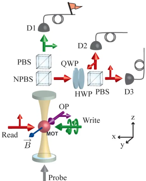
Atomic quantum memory for photon polarization
Texte intégral
Figure


Documents relatifs
predict the transition pressure between ferromagnetic and non- magnetic states, we have increased pressure on these compounds until the extinction of the magnetic moment and appear
In the quantum regime, single photons generated by an ensemble of cold atoms via DLCZ have been reversibly mapped with an efficiency of around 50 % into another cold atomic ensemble,
2014 A strong degree of polarization (64 %) has been observed in the fluorescence from calcium atoms excited by the photodissociation of Ca2 molecules in their ground
In its most efficient form, namely using the gradient echo memory scheme (GEM) [16] (sometimes called longitudinal CRIB) or using (transverse-) CRIB with a backward write pulse
Keywords: quantum optics, quantum information, continuous variables, quantum memory, optical parametric oscillator, squeezed states, entanglement, quantum tomog-
Thus, 10 hospital laboratories with expertise in culture of Legion- ella species performed both prospective and retrospective surveys of Legionella species isolated from the
Le problème de la répartition optimale des puissances est un problème d’optimisation dont l’objectif est de minimiser le coût total de la production de la puissance d’un
Vitesse de disparition d’un réactif et de formation d’un produit ; lois de vitesse pour des réactions d’ordre 0, 1, 2… ; ordre global, ordre apparent ; Temps de
