Comparison of four models to rank failure likelihood of individual pipes

Publisher’s version / Version de l'éditeur:

Vous avez des questions? Nous pouvons vous aider. Pour communiquer directement avec un auteur, consultez la

première page de la revue dans laquelle son article a été publié afin de trouver ses coordonnées. Si vous n’arrivez pas à les repérer, communiquez avec nous à PublicationsArchive-ArchivesPublications@nrc-cnrc.gc.ca.

Questions? Contact the NRC Publications Archive team at

PublicationsArchive-ArchivesPublications@nrc-cnrc.gc.ca. If you wish to email the authors directly, please see the first page of the publication for their contact information.

https://publications-cnrc.canada.ca/fra/droits

L’accès à ce site Web et l’utilisation de son contenu sont assujettis aux conditions présentées dans le site

LISEZ CES CONDITIONS ATTENTIVEMENT AVANT D’UTILISER CE SITE WEB.

Journal of Hydroinformatics, 14, 3, pp. 659-681, 2012-06-01

READ THESE TERMS AND CONDITIONS CAREFULLY BEFORE USING THIS WEBSITE. https://nrc-publications.canada.ca/eng/copyright

NRC Publications Archive Record / Notice des Archives des publications du CNRC : https://nrc-publications.canada.ca/eng/view/object/?id=cea030fd-fba6-49a3-9b88-017dd7e0c3f2 https://publications-cnrc.canada.ca/fra/voir/objet/?id=cea030fd-fba6-49a3-9b88-017dd7e0c3f2

Archives des publications du CNRC

This publication could be one of several versions: author’s original, accepted manuscript or the publisher’s version. / La version de cette publication peut être l’une des suivantes : la version prépublication de l’auteur, la version acceptée du manuscrit ou la version de l’éditeur.

For the publisher’s version, please access the DOI link below./ Pour consulter la version de l’éditeur, utilisez le lien DOI ci-dessous.

https://doi.org/10.2166/hydro.2011.029

Access and use of this website and the material on it are subject to the Terms and Conditions set forth at

Comparison of four models to rank failure likelihood of individual pipes Kleiner, Y.; Rajani, B. B.

Comparison of four models to

rank failure likelihood of

individual pipes

Kleiner, Y.; Rajani, B.B.

NRCC-55236

A version of this document is published in Journal of Hydroinformatics, 14, (3), pp. 659–681,2012-06-01, DOI: 10.2166/hydro.2011.029

The material in this document is covered by the provisions of the Copyright Act, by Canadian laws, policies, regulations and international agreements. Such provisions serve to identify the information source and, in specific instances, to prohibit reproduction of materials without

written permission. For more information visit http://laws.justice.gc.ca/en/showtdm/cs/C-42

Les renseignements dans ce document sont protégés par la Loi sur le droit d’auteur, par les lois, les politiques et les règlements du Canada et des accords internationaux. Ces dispositions permettent d’identifier la source de l’information et, dans certains cas, d’interdire la

Yehuda Kleiner and Balvant Rajani

National Research Council Canada, Ottawa, Ontario, Canada

Abstract

The use of statistical methods to discern patterns of historical breakage rates and use them to predict water main breaks has been widely documented. Particularly challenging is the prediction of breaks in individual pipes, due to the natural variations that exist in all the factors that affect their deterioration and subsequent failure. This paper describes alternative models developed into operational tools that can assist network owners and planners to identify individual mains for renewal in their water distribution networks. Four models were developed and compared: a heuristic model, naïve Bayesian classification model, a model based on logistic regression and finally a probabilistic model based on the Non Homogeneous Poisson Process (NHPP). These models rank individual water mains in terms of their anticipated breakage frequency, while considering both static (e.g., pipe material, diameter, vintage, surrounding soil, etc.) and dynamic (e.g., climate, operations, cathodic protection, etc.) effects influencing pipe deterioration rates.

Key words: heuristic, logistic regression, naïve Bayesian classification, non-homogeneous Poisson process, pipe break forecast, ranking

Introduction

The use of statistical methods to discern patterns of historical breakage rates and use them to predict water main breaks has been widely documented. Kleiner and Rajani (2001) provided a comprehensive review of approaches and methods that had been developed prior to their review. Since then, several more methods have been proposed, such as those by Dandy and Engelhardt (2001), Park and Loganathan (2002), Mailhot et al. (2003), Jarrett et al. (2003), Dridi et al. (2005), Giustolisi et al. (2005), Watson et al. (2004), Giustolisi and Berardi (2007), Boxall et al. (2007), Le Gat (2008) and Economou et al. (2008) to name but a few. In all these methods, few, if any, heuristic methods have been documented to discern patterns of historical breakage rates.

Many factors, operational, environmental and pipe-intrinsic factors, jointly affect the breakage rate of a water main. While not all pipes are created equal (even pipes of the same material and size), it is normally assumed that pipes that share specific intrinsic properties, such as material, diameter, vintage, etc., can be expected to have the same breakage pattern, all else being equal. However, non-pipe-intrinsic factors may have varying effects on the breakage patterns of different pipes, even if all else is equal. For example, two pipes of the same material, diameter, age, etc., can be impacted differently by climate. We may never have enough data to account for these differences due to variability. At the same time, it is unreasonable to perform a statistical analysis on the breakage pattern of a single pipe because sufficient data on breaks to conduct a credible analysis are not available. For these reasons, the forecasting of breaks in individual water mains has proven to be quite a challenge.

This paper describes four specific models intended to serve as operational tools for water distribution network owners and planners to help them rank individual water mains for renewal, while considering both static (e.g., pipe material, diameter, vintage, surrounding soil, etc) and dynamic (e.g., climate, operations, cathodic protection, etc.) effects influencing pipe

deterioration rates. It should be noted that risk-based prioritization of water mains for renewal, entails the quantification of both likelihood and consequences of failure. However, this research focused only on failure likelihood, and therefore in this paper the word “ranking” refers strictly to failure likelihood-based ranking.

Four models were developed and compared; a heuristic model named “Ordered Lists” (OL), comprising procedures that reflect intuition and observations, a model based on naïve Bayesian classification (NBC), one based on logistic regression and finally a probabilistic model based on the Non Homogeneous Poisson Process (NHPP). The first three are the so-called “ranking” models, intended for forecasting, within a homogeneous group, the ranking of individual pipes in terms of their relative failure likelihood, rather than attempt to forecast the actual number of breaks. The rationale was that the existing statistical/empirical models (such as D-WARP – see Kleiner and Rajani, 2004) forecast the aggregate breakage rate for a homogeneous group of pipes, the ranking models would be useful to drill down to the individual pipe level within the group (note that D-WARP considers both static and dynamic effects impacting pipe breakage rate). The fourth model is different from the first three in that it actually endeavours to forecast future breakage rates of individual pipes, rather than just rank them on relative failure likelihood.

The ranking models were set out to address the following challenge: “In a homogeneous group

comprising N individual pipes, with available breakage history of T years, find which n

pipes are expected to have the highest number of breaks in the next y years”. The rest of this paper is organized as follows. We first describe the covariates that were examined and used for the ranking models. Some of these covariates are new in the context of pipe breakage analysis and are based on practical observations and heuristic arguments. Subsequently, the three ranking models are described with details on how these and other covariates were used to rank individual mains. In the interest of good readability, some of the lengthy formulations are provided in appendices A, B and C rather than in the main text. The last model introduced is based on NHPP. The comparison between the four models is presented next by way of an example dataset, followed by some concluding comments.

Covariates for the ranking models

Pipe length. In practice all reported analyses of breakage frequency in pipe groups, aggregate

length of a group has been used as a normalizing factor (e.g., Shamir and Howard, 1979; Walski and Pelliccia, 1982; Clark et al., 1982; Kettler and Goulter, 1985; Kleiner and Rajani, 2004 and others). This has the implication that breaks are distributed uniformly along the pipes, which carries the expectation that the number of breaks is directly proportional to the length of pipes. This implication has been questioned by others, e.g., Goulter and Kazemi (1988), Goulter et al. (1993), Jacobs and Karney (1994) and Mavin (1996).

The literature reflects that pipe length has frequently been used as a covariate to “explain” at least some of the variability observed in individual water mains. Andreou et al. (1987), Eisenbeis

et al. (1999), Røstum (2000), Le Gat and Eisenbeis (2000) and others used the log of pipe length

as a covariate in their proportional hazards-based models (PHM).

The researchers cited above reported various outcomes with respect to the “quality” of pipe length as a covariate. In some water distribution networks, length was found to be statistically significant, while in others it was not. Additionally, in some pipe materials (cast iron (CI), PVC) length was found to be significant when the number of previous breaks was between 1 and 3, while insignificant when the number of previous breaks was zero or equal to or greater than 4. In other materials (asbestos cement (AC)) it was found to be not significant at any level of previous breaks. In some cases the square root of the pipe length was found to be a significant covariate.

The dichotomy of using length as a normalizing factor, as well as the inconclusive results using length as covariate, triggered an investigation, details of which are reported by Kleiner and Rajani (2010). They conclude that pipe length is a surrogate for pipe exposure and higher exposure necessarily leads to more breaks. However, the natural randomness inherent in the relationship between length and breaks is relatively high. Further, pipe break is a discrete entity while pipe length is a continuous physical property. Individual pipes, whose length might typically vary between a few tens and a few hundreds of meters, typically do not experience too many breaks before they are replaced. This discrete nature of breakage data amplifies the natural randomness in relatively short pipes. Consequently, the randomness or the “noise” in the data often overwhelms any mathematical relationship that may exist between length and observed breakage rate. However, when aggregated pipe lengths are examined, the aggregate number of breaks becomes continuous-like in their behaviour and the natural randomness produces “noise” that is much smaller relative to the mathematical relationship and therefore no longer

overwhelms this relationship. Furthermore, it appears that the relationship between breakage rates and length of individual water mains can be better characterized as non-parametric but monotone. This was revealed by rank correlation analyses, which consistently yielded better results than linear correlation.

Breakage history: number of known previous failures (NOKPF). The essence of all

statistical/empirical pipe failure prediction models is to use failure history to discern failure patterns. Therefore, these models always use the number of previous failures (NOPF) either explicitly or implicitly. In PHM it can be used as a covariate or as a stratification criterion (e.g., Andreou et al., 1987). In the past, NOPF has not been used explicitly as a covariate in non homogeneous Poison process (NHPP) models. Gustafson and Clancy (1999) and Mailhot et al. (2003) used break order (e.g., 1st break, 2nd break since installation, etc.) as a stratification criterion of sorts, upon which distribution parameters of time to failure are dependant. It should be recognized that in reality, most water utilities will have left-truncated datasets because they do not have pipe failure data that covers the entire history of pipes since installation (except for recently installed pipes). For this reason, models that use break order as a parameter will find little applicability. Also for this reason we chose to name this candidate covariate

number of known previous failures (NOKPF) as opposed to the more commonly used number of previous failures (NOPF).

Breakage history: Recency. Recency expresses the tendency of historical breaks to have occurred

more towards the beginning or towards the end of the observation period. Recency is defined with the use of Figure 1. T is the observation period, which starts at t0 and ends at te. t1 denotes

the time (since t0) of the first break recorded for this pipe, t2 is the time of second break, and so

forth. The pipe in Figure 1 experienced a total of b breaks during period T. The Recency (Rei) of

breakage pattern of pipe i during a historical observation period T is defined as follows

0 ; 1 1 1 1 > = =

∑

∑

which pipe i experienced its j-th break (t is measured from _ij t ). ₀ R is defined as zero when e_i

0 =

i

b (no breaks in period T). It is clear that 0≤Re_i ≤1. Thus, lower values of Recency mean that the observed historical breaks tend to have occurred more towards the beginning of the observation period, whereas higher values indicate breaks have occurred more recently.

Figure 1. Timeline for definitions of Recency and Scatter

Breakage history: Scatter. There are several ways to represent how observed historical breaks are

concentrated (or scattered) through the observation period. Two different formulations were examined, one based on the square deviation from the mean breakage year and the other based on Shannon’s entropy. No consistent differences in model performance were observed between the two formulations and Shannon’s entropy was selected for convenience. The Scatter (Sci) of

breakage pattern of pipe i during a historical observation period T is defined as follows (Figure 1):

i i i b e b i j i ij ij i b j ij ij i i t t w T t t w b w Ln w b Ln Sc − = − = > + − = + − + =

∑

It can be shown that when all breaks are evenly spaced along T then Sc=1. Also when all breaks are concentrated at t or at ₀ t then _e Sc=0. When all points are concentrated exactly in the middle of historical observation period T, then Sc=2 Ln

(

)

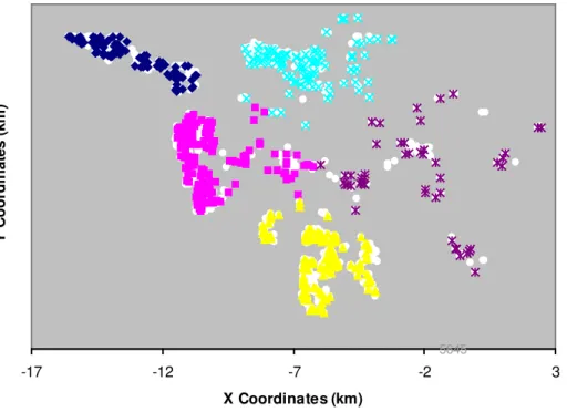
Geographical clustering. Water utilities often lack data that are geographically related (directly

or indirectly), such as soil data, overburden characteristics (land development, traffic patterns), historical installation practices, groundwater fluctuations, transient pressures, poor bedding, etc. These data, if available, may sometimes help “explain” variations in breakage rates among individual water mains in a “homogeneous” group of pipes. In the absence of such data, the proximity of a pipe to a cluster of historical breaks may serve as a useful surrogate.

The K-Means algorithm (MacQueen, 1967) was used to create the Cluster covariates (or

Clusters). Given n data points and K centroids (cluster centres), this algorithm assigns each data

point to the nearest centroid, then recalculates and shifts the location of the centroid and again re-assign each data point to the new location of the centroid, and so forth until equilibrium is reached and the centroids no longer shift their locations. The K-Means algorithm is capable of clustering multi-dimensional (or multi attribute) data. The application to two-dimensional geographical data (only X and Y coordinates) is therefore relatively simple and fast. In anticipation of typical availability of such geographical data, it was deemed sufficiently accurate to assume that the location of a break is always at the centre of the pipe (which can be computed from the pipe-node coordinates). It should be noted that the K-Means clustering algorithm does not determine the optimal number of clusters or their approximate locations, rather the user needs to visually determine those based on observation of historical break locations as well as on prior knowledge.

Figure 2 illustrates an example of clusters. Breaks and pipes were arbitrarily (visually) divided into five clusters, represented by five different colour dots, dark blue, light blue, yellow and purple. The grey dots in the background represent the centres of all pipes in the group (obviously not all pipes experienced breaks in this period).

Ordered lists (OL) model

The Ordered lists (OL) model is essentially a weighted, non-parametric heuristic model,

and anticipated breakage frequency in individual water mains. The model comprises two sub-procedures, model training (or calibration) and model validation. Model validation is conducted on a “holdout” sample data.

Figure 2. LogReg example – Spatial distribution and clustering of pipes and breaks. Procedure for model training

a. Partition the observation period T into training and validation periods, where the validation period comprises the latest v years in T (Figure 3).

Figure 3. Timeline for training and validation procedure

b. Select RefYear and partition the training period into WinPast and WinFuture. Identify n pipes with the highest number of breaks in period WinFuture and WinValidation. Record these pipes in lists named L and_f L , respectively. _v

Training period

te

t0

WinPast WinFuture WinValidation

RefYear Validation period T 5645 -17 -12 -7 -2 3 X Coordinates (km) Y C o o rd in at es ( km )

c. Create an ordered listL , containing all pipes sorted by the covariate NOKPF (number of _b

known previous failures) observed during WinPast in descending order (pipe with highest past breaks ranks first, etc.).

d. Similar to c. above, create an ordered listL , containing all pipes sorted by length in _l

descending order (longest pipe first, etc.).

e. Similar to c. above, create an ordered listL , containing all pipes sorted by Recency during _R WinPast in descending order (highest Recency first, etc.).

f. Similar to c. above, create an ordered listL , containing all pipes sorted by Scatter during _S WinPast in descending order (highest Scatter first, etc.).

g. Assign weights W_b,W_l,W_R,W_Sto listsL_b,L_l,L_R,L_S, respectively. Each list represents a covariate and each covariate is associated with a weight.

h. For each pipe i in the group, compute a composite score Cs that combines the rank _i R of _iL

this pipe in each list and the corresponding weight: ) , , , , , , , ( _iL _iL _iL _iL _{b l R S} i f R R R R W W W W Cs = b l R S ₍₃₎ where Lb i

R represents the rank of pipe i in list L , etc., and f(_b .) is an aggregation function. Several different types of aggregation functions were tested as described later.

i. Rank all pipes by their composite scores in ascending order (lower score corresponds to lower order rank, which means higher breakage potential). The n pipes with the lowest scores are those predicted by the model to have the highest number of breaks in the future window. Record these pipes in a listL . _w

j. Compare listL to list_w L . If a certain pipe i appears in both lists (irrespective of location _f

within a list) this occurrence is defined as a “hit”. Determine the number of hits, H.

k. Find a set of weights (W_b*,W_l*,W_R*,W_S*) that maximizes H. We then say that the model has been trained on the group of pipes that meets this condition. We used genetic algorithm (simple, single objective GA, using binary coded genes, crossover and mutation operators and roulette wheel-based selection mechanism) to maximize H.

Note that the Cluster covariate, which is a categorical covariate was not used in the Ordered lists model. It can be used, however, by partitioning the pipes in the group into subgroups

Procedure for model validation

For simplicity, we define WinPastValidation = WinPast + WinFuture. T is now partitioned into

WinPastValidation and WinValidation (Figure 3).

i. Repeat training steps c. through g. to create new ordered lists – “validation” lists

S R l

b L L L

L′, ′ , ′, ′ . For lists L_b′,L_R′,L_S′ use the time period WinPastValidation. Note thatL′ , _l

which refers to pipe length is the same as L (pipe lengths do not change). _l

ii. Apply the weights (W_b*,W_l*,W_R*,W_S*) to the validation lists and repeat training steps i. and j., where the n pipes with the lowest scores are recorded in listL′ . The list _w L′ contains _w

pipes predicted by the model to have the highest number of breaks in the validation time window. Note that the observed breaks in the validation time period (holdout sample data) did not participate in the training of the model.

iii. Determine,H ′ , the number of hits (pipes that appear in both lists) in lists L′ and_w L . _v

iv. Repeat the validation process for various n values (where n is the number of pipes with the highest breakage rates – see training step i.). Use the method described in Appendix A to analyze results.

Aggregation functions. As the Ordered lists model is a heuristic procedure, it is not possible to

determine a priori what type of aggregation function will best be suited for a specific dataset. Consequently, seven different published aggregation functions were tested. These functions can be classified into three classes, “Cardinal”, “Ordinal” and “Mixed” weights. The Cardinal weights class comprises aggregation functions in which each weight is assigned specifically to a covariate (list), exactly as described in training step h. above. In this class we included two specific functions, CardIndepend and CardDepend. The Ordinal weights class comprises aggregation functions in which a weight is assigned to a covariate based on the relative ranking that this covariate has for a given pipe. In this class we included four functions; OrdMaxMin,

OrdMaxNext, OrdAll and OrdChoquet. The Mixed weights class comprises one function Mixed,

which involves a combination of cardinal and ordinal weights. A description of the aggregation functions, as well as their precise mathematical formulations are provided in Appendix B.

Example. A homogenous group of CI pipes from Calgary was analyzed, including 1091 pipes (146.6 km or 91 miles total length), 150 mm (6”) in diameter, installed between 1956 and 1960,

and each pipe was at least 20 m long. Full year breakage data were available for the years 1961 - 2006. The OL model was trained on 40 years failure data from 1962 to 2001, where WinPast was taken as 35 years (1962 - 1996), WinFuture was taken as 5 years (1997 – 2001) and

WinValidation was taken as 5 years (2002 – 2006). RefYear is accordingly 1996. The weights

obtained from training (calibration) were used to forecast the ranking of pipes in the validation period. The model was trained on several n values that were selected to correspond to the number of pipes in the group observed with a precise number of breaks. The results are summarized in Tables 1 through 4. Note that the results for the same aggregation function can vary through multiple runs (a “run” refers to a training and validation session) because training is done using genetic algorithm, which is a search heuristic with random elements. Consequently, the model was applied 16 times with each aggregation function. The result tables provide the minimum, maximum and average number of training hits (in 16 runs), as well the minimum, maximum and average number of validation hits (note that in the training period a maximum of 3 breaks was observed in any given pipe, while in the validation periods up to 4 breaks were

observed) . Note further that P-values were used (Tables 2 and 4) to assess the ranking ability of the model for a given dataset. Appendix A describes in detail how these P-values are computed.

Table 1. Summary of Ordered lists (OL) model example results (number of hits) - training

Number of pipes recorded with at least

1 break 2 breaks 3 breaks 4 breaks

Aggregation function 138 24 6 0

Max. 46 3 1

Cardinal / independent Min. 44 1 0

Mean 45.2 2.1 0.8

Max. 48 5 1

Cardinal / with dependencies Min. 44 0 0

Mean 45.2 1.9 0.4

Max. 39 2 1

Ordinal / Max. & min. Min. 39 2 1

Mean 39.0 2.0 1.0

Max. 42 4 1

Ordinal / Max. & next Min. 42 4 1

Mean 42.0 4.0 1.0

Max. 43 4 1

Ordinal / All Min. 42 2 0

Mean 42.3 3.9 0.4

Max. 43 5 1

Ordinal / Choquet Min. 42 4 0

Mean 42.4 4.1 0.8

Max. 43 5 1

Mixed weights Min. 42 4 0

Mean 42.7 4.1 0.9

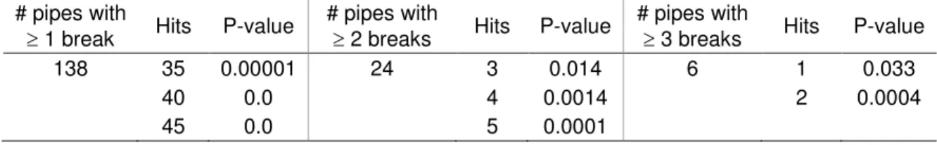
Table 2. Summary of Ordered lists (OL) model example results – training P-values (total 1091 pipes in sample)

# pipes with

≥ 1 break Hits P-value

# pipes with

≥ 2 breaks Hits P-value

# pipes with

≥ 3 breaks Hits P-value

138 35 0.00001 24 3 0.014 6 1 0.033

40 0.0 4 0.0014 2 0.0004

Table 3. Summary of Ordered lists (OL) model example results (number of hits) - validation

Number of pipes recorded with at least

1 break 2 breaks 3 breaks 4 breaks

Aggregation function 170 30 6 2

Max. 54 7 2 0

Cardinal / independent Min. 49 6 0 0

Mean 51.4 6.4 1.1 0

Max. 55 7 1 0

Cardinal / with dependencies Min. 44 1 0 0

Mean 49.3 4.2 0.4 0

Max. 52 9 1 1

Ordinal / Max. & min. Min. 46 5 1 0

Mean 47.3 5.7 1.0 0.9

Max. 52 7 1 1

Ordinal / Max. & next Min. 52 7 1 1

Mean 52.0 7.0 1.0 1.0

Max. 53 8 2 1

Ordinal / All Min. 45 5 0 0

Mean 50.3 7.0 1.3 0.3

Max. 55 8 2 1

Ordinal / Choquet Min. 50 6 1 0

Mean 52.0 7.2 1.8 0.6

Max. 55 8 2 1

Mixed weights Min. 50 7 1 0

Mean 51.6 7.2 1.9 0.2

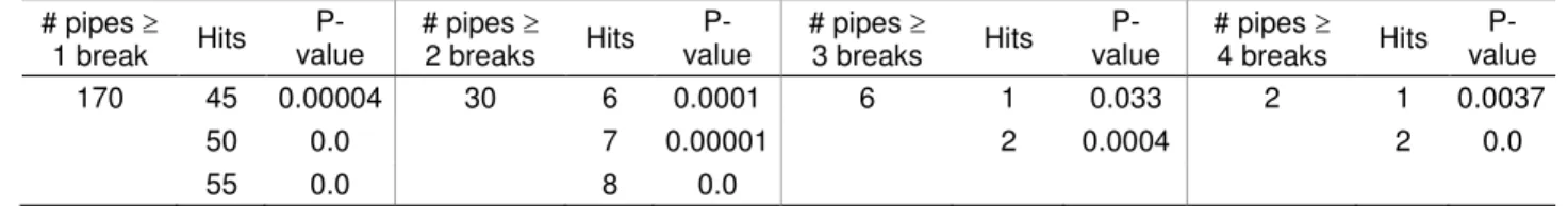
Table 4. Summary of Ordered lists (OL) model example results - validation P-values (total 1091 pipes in sample) # pipes ≥ 1 break Hits P-value # pipes ≥ 2 breaks Hits P-value # pipes ≥ 3 breaks Hits P-value # pipes ≥ 4 breaks Hits P-value 170 45 0.00004 30 6 0.0001 6 1 0.033 2 1 0.0037 50 0.0 7 0.00001 2 0.0004 2 0.0 55 0.0 8 0.0

The application of the OL models on the example dataset shows that it could be trained to identify about one third of all the pipes that experienced at least one break in the WinFuture period, as well as about 10% to 15% of the pipes that experienced at least two breaks and about 0% to 15% of pipes with at least three breaks. It is also noted that in this dataset there were no

significant differences between the training (calibration) success rates of the various aggregation functions.

In the validation session, the OL model only succeeds to identify less than one third of all the pipes that experienced at least one break in the WinValidation period, as well as about 20% to 30% of the pipes that experienced at least two breaks, about 0% to 30% of pipes with at least three breaks, and 0% to 50% of pipes with at least four breaks. As noted in the training session, no significant difference between the forecasting success rates of the various aggregation functions is seen in this dataset (this could differ in other datasets).

Naïve Bayesian Classification (NBC) model

The naïve Bayesian classification method is based on Bayes’ rule and uses attributes (or

covariates or classifiers) to partition data into pre-defined classes. The underlying assumption in the NBC model is that these covariates are conditionally independent of one another (i.e., if the class is known then the covariates are statistically independent of each other) and ignores possible interactions between attributes (covariates). Denoting X₁,X₂,,X_J

as covariates and

Y as the outcome (or class), which in our case is binary (0/1), Bayes’ rule can be stated as

) , , , Pr( ) Pr( ) | , , , Pr( ) , , , | Pr( 2 1 2 1 2 1 j j j X X X Y Y X X X X X X Y    = ₍₄₎

where the expression on the left denotes posterior probability, the numerator on the right is the product of likelihood and prior probability and the denominator denotes evidence. Usually only the numerator is of interest because the denominator does not depend on Y. Using the conditional independence assumption described above, it can be shown that the likelihood function becomes

∏

and therefore the conditional probability of outcome Y becomes

∏

When the response (Y) is binary, as in our case, we can simplify by computing the so-called likelihood ratio (LR).

∏

∏

∏

The likelihood ratioLR for each pipe i in the homogeneous group is calculated and subsequently _i

the pipes are sorted in ascending LR order. The n highest ranked pipes on the list are those with the highest likelihood to break. The calculations are simplified by ranking the pipe according to their Ln(LR)since the Ln of LR is monotone, i.e.,:

∑

Continuous covariates (Length, Recency, Scatter) as well as discrete covariate (NOKPF) have to be converted to classes (or bins) in order to evaluateLn(LR_i). Consequently, these covariates were converted to classes such as Very high (VH), High (H), Medium (M), Low (L) and Very low (VL), where each class is defined by lower and upper bounds for each covariate. Complete details are provided in Appendix C.

Procedure for model training

The training part of this NBC model is to find lower and upper bounds for covariates that maximize the number of hits. The procedure for training is:

Training steps a. and b. are identical to training steps a. and b. in OL training.

c. For every pipe i in the group Yi = 1 if it is among the n highest breaking pipes during

WinFuture period. Otherwise Yi = 0.

d. Establish bins (classes), e.g., Very high (VH), High (H), Medium (M), Low (L) and Very low (VL), for every covariate, as is described in Appendix C. These bins are established by specifying their lower and upper bounds for each covariate. Note that the Cluster covariate is by nature a class covariate and therefore does not require any transformation. e. Transform all covariates (except Cluster) to class covariates for every pipe in the group

f. Rank all pipes byLR in descending order (i.e., pipes with the highest likelihood of (Y = 1) _i

are ranked highest. The n highest ranked pipes are those predicted to have the highest number of breaks in the future window WinFuture. Record these pipes in a listL . _w

g. Compare list L to list_w L . If a certain pipe i appears in both lists (irrespective of location _f

within a list) this occurrence is defined as a “hit”. Determine the number of hits, H. h. Find a set of lower and upper bin bounds that maximizes H. We used genetic algorithm to

maximize H.

Procedure for model validation

i. Repeat training step e., but use WinPastValidation instead of WinPast.

ii. Repeat training step f., but use WinPastValidation instead of WinPast (use bin boundary values that were found in training step h. above).

iii. Repeat training step g., but use WinValidation instead of WinFuture. Record these pipes in a listL′ . The list _w L′ contains pipes predicted by the model to have the highest number of _w

breaks in the validation time window. Note that the validation time period did not participate in the training of the model, hence it is a holdout sample.

iv. Determine, H ′ , the number of hits that appear in both listsL′ and _w L . _v

v. Repeat the validation process for various n values (where n is the number of pipes with the highest breakage rates – see training step f. Use the method described in Appendix A, to evaluate results.

Example. The same dataset used for the OL model above is employed here to demonstrate the application of the naïve Bayesian classification method. The periods used to define WinPast,

WinFuture and WinValidation for the OL model were also used for the NBC model. Three

separate training and validation sessions were carried out, namely, for identifying pipes with at least one break, at least two breaks and at least three breaks. Note that this example cannot be trained to identify at least four breaks because no pipes were observed with more than three breaks in the WinFuture time period. Results are presented in Tables 5 through 7. It is interesting to note that the lower and upper bounds vary, sometimes significantly, among the three training sessions. It should also be remembered that the bounds are found using GA so as to maximize

the number of training hits. Running the same training sessions several times consecutively will produce results that will often vary from each other since GA is a search heuristic with random elements. As can be expected, P-values of the training sessions are generally better than

validation.

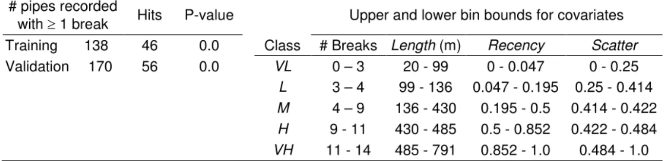
Table 5. NBC model example results – training and validation for pipes with at least 1 break. # pipes recorded

with ≥ 1 break Hits P-value Upper and lower bin bounds for covariates Training 138 46 0.0 Class # Breaks Length (m) Recency Scatter

Validation 170 56 0.0 VL 0 – 3 20 - 99 0 - 0.047 0 - 0.25

L 3 – 4 99 - 136 0.047 - 0.195 0.25 - 0.414

M 4 – 9 136 - 430 0.195 - 0.5 0.414 - 0.422

H 9 - 11 430 - 485 0.5 - 0.852 0.422 - 0.484

VH 11 - 14 485 - 791 0.852 - 1.0 0.484 - 1.0

Table 6. NBC model example results – training and validation for pipes with at least 2 breaks. # pipes recorded

with ≥ 2 breaks Hits P-value Upper and lower bin bounds for covariates Training 24 8 0.0 Class # Breaks Length (m) Recency Scatter

Validation 30 3 0.046 VL 0 - 2 20 - 346 0 - 0.445 0 - 0.086

L 2 - 3 346 - 394 0.445 - 0.555 0.086 - 0.367

M 3 - 7 394 - 479 0.555 - 0.625 0.367 - 0.484

H 7 - 12 479 - 599 0.625 - 0.961 0.484 - 0.93

VH 12 - 14 599 - 791 0.961 - 1.0 0.93 - 1.0

Table 7. NBC model example results – training and validation for pipes with at least 3 breaks. # pipes recorded

with ≥ 3 breaks Hits P-value Upper and lower bin bounds for covariates Training 6 3 0.0 Class # Breaks Length (m) Recency Scatter

Validation 6 1 0.033 VL 0 - 4 20 - 195 0 - 0.438 0 - 0.156

L 4 - 7 195 - 202 0.438 - 0.46 0.156 - 0.195

M 7 - 11 202 - 256 0.46 - 0.805 0.195 - 0.297

H 11 - 12 256 - 358 0.805 - 0.859 0.297 - 0.664

Logistic regression (LogReg) model

Logistic regression investigates how well a set of independent (explanatory) variables can explain the value of a dichotomous dependent variable. In our model the dichotomous dependent variable Y is whether the pipe belongs to the n highest breaking pipes in the next y years (Y = 1) or does not belong (Y = 0). The independent (explanatory) variables can be NOKPF, Length,

Cluster, Recency and Scatter, where each can be taken either in their parametric form (numerical

value) or non-parametric form (ordinal value or relative rank). Cluster covariates can also be considered in the form of binary covariates (i.e., each cluster is represented by a 0/1 value, but the sum of all Cluster covariates equals unity). The probability that pipe i belongs to the n highest breaking pipes using the logistic function is expressed by

x β x β e e Yi i + = = 1 ) 1 ( Pr (9)

where x is a vector of covariates (or explanatory variables) and β is a vector of coefficients to be found by maximum likelihood. The likelihood function l for N observations (= N pipes in the group) can be expressed by

∏

and the log-likelihood is therefore

∑

As before, the procedure to identify the n highest breaking pipes is divided into two sub-procedures, model training and model validation. Model validation is conducted on a holdout sample.

Procedure for model training

The modelling training process is as follows.

Training steps a., b. and c. are identical to training steps a., b. and c. in NBC training.

d. For every pipe in the group, establish the covariates (explanatory variables) x. These could be for example, actual NOKPF during WinPast, Length, Recency during WinPast and Scatter during WinPast. These covariates could be taken at their numerical values or alternatively at their rank value or combinations of ranks and numerical values.

e. Cluster covariate, as described earlier, is taken as a categorical covariate. If the pipe in the group are partitioned into K clusters then K binary (zero/one) covariates are assigned, one to each cluster, with corresponding k coefficients, where the sum of these K covariates must equal unity. For example, a model that has i parametric covariates and K = 3 categorical covariates is described by (categorical covariates in the square brackets)

[

]

f. Perform the logistic regression and find coefficients β by maximizing the log-likelihood function.

g. Apply β to the covariates in WinPast and obtain Pri for each pipe i.

h. Rank all pipes by Pri in descending order (i.e., pipes with the highest probability of (Y = 1)

are ranked highest. The n highest ranked pipes are those predicted to have the highest number of breaks in the future window WinFuture. Record these pipes in a listL . _w

i. Identical to training step g. in NBC training.

Procedure for model validation

Recall that for simplicity we define WinPastValidation = WinPast + WinFuture. T is now partitioned into WinPastValidation and WinValidation (Figure 3).

i. Repeat training steps d. and e., but use WinPastValidation instead of WinPast.

ii. Repeat training step g., but use WinPastValidation instead of WinPast (use β values that were found in training step f. above).

iii. Repeat training step h., but use WinValidation instead of WinFuture. Record these pipes in a list L′ . The list _w L′ contains pipes predicted by the model to have the highest number of _w

breaks in the validation time window. Note that the validation time period did not participate in the training of the model, hence it is a holdout sample.

iv. Determine,H ′ , the number of pipes (hits) that appear in both lists L′ andw L . v

v. Repeat the validation process for various n values (where n is the number of pipes with the highest breakage rates – see training step g.). Use the method described in Appendix A to evaluate results. 1 ; 1 / 0 , , _{2 3 1 2 3} 1 + + = + + + + + = + i i i i i i x x x x x x

Example. The same dataset used for testing OL and NBC models earlier is used to demonstrate the LogReg model. However, geographical data for pipes (Figure 2) was added to form the Cluster covariate. The periods used to define WinPast, WinFuture and WinValidation for the OL and NBC models were used for the LogReg model. Potential covariates include NOKPF, BreakRate

(= NOKPF/Length), Length, Recency, Scatter and Clusters. Each of the physical covariates (i.e., all except Clusters) can be considered either at its numerical value or at its rank value. Therefore, there are altogether 11 potential covariates (5 values, 5 ranks and one that corresponds to Clusters). The model can be run with numerous different combinations of covariates.

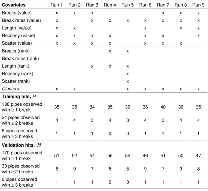
Table 8 provides results for 9 different runs with different combinations of covariates. Each run in fact comprises three training sessions, to identify pipes with at least one or two or three breaks in their known history. It can be seen that the highest training results do not necessarily lead to the highest validation results. It can also be seen that none of the covariate combinations are clearly superior or inferior to the rest.

Non Homogeneous Poisson Process based model

Non homogeneous Poisson process (NHPP) has been suggested by several researchers to model and forecast water main breaks (e.g., Constantine and Darroch, 1993; Constantine et al., 1996; Røstum, 2000; Jarrett et al., 2003; Economou et al., 2008, among others). The approach proposed here differs from others in that it allows for the consideration of dynamic factors (climate, operations, etc.), while existing NHPP approaches consider only pipe-intrinsic, static factors (diameter, length, material, etc.). The proposed NHPP-based model is in a different class compared to the three ranking models described earlier, in that it endeavours to forecast actual breakage rates in individual water mains, rather than just rank their relative rates.

In the proposed model, breaks at year t for an individual pipe i are assumed to be Poisson arrivals with mean intensity (or mean rate of occurrence)λ_i,t. Therefore, the probability of observing k_i,t

breaks is given by:

! ) exp( ) Pr( , , , , , t i t i k t i t i k k t i λ λ ⋅ − = where λ_i,t =exp[α_o +θτ(g_i,t)+αzi +βpt +γqi,t] (12)

Table 8. LogReg model example results – training and validation with various covariates.

Covariates Run 1 Run 2 Run 3 Run 4 Run 5 Run 6 Run 7 Run 8 Run 9

Breaks (value) x x x x x x

Break rates (value) x x x x x x x x

Length (value) x x x x x

Recency (value) x x x x x x x

Scatter (value) x x x x x x x

Breaks (rank) x x

Break rates (rank)

Length (rank) x x x Recency (rank) x Scatter (rank) x Clusters x x x x x x x Training hits, H 138 pipes observed with ≥ 1 break 35 35 34 35 39 36 40 36 35 24 pipes observed with ≥ 2 breaks 4 4 3 4 3 4 3 4 4 6 pipes observed with ≥ 3 breaks 1 1 1 0 0 1 1 1 1 Validation hits, H ′ 170 pipes observed with ≥ 1 break 51 52 54 56 55 46 51 50 47 30 pipes observed with ≥ 2 breaks 8 9 7 5 5 9 7 9 8 6 pipes observed with ≥ 3 breaks 1 1 1 0 0 1 1 1 1

and where α_ois a constant, τ(gi,t)is the age covariate, and θ is its coefficient, gi,tis the age of

pipe i at year t;z is a row vector of pipe-dependent covariates (e.g., length, diameter, etc.) and i α

is a column vector of corresponding coefficients;p is a row vector of time-dependent covariates t

(e.g., climate) and β is a column vector of corresponding coefficients; qi,tis a row vector of both pipe-dependent and time-dependent covariates (e.g., number of known previous failure -

NOKPF, cathodic protection) and γ is a column vector of corresponding coefficients. In this paper, the functionexp[θτ(g_i,t)] is referred to as the “ageing function” and therefore coefficient θ is called “ageing coefficient”. Note that if τ(g_i,t)=g_i,tthen the ageing is exponential, i.e., λ is

power function, i.e., λ becomes a power function of pipe age. Year t is taken relative to the first year for which breakage records are available. The likelihood function for (12) is

∏∏

) ! ln( ) ln( _{, ,} 1 1 , , it it N i T t t i t i k k LL=

∑∑

Covariates of the NHPP model

Pipe-dependent covariates. Pipe-dependent covariates can be considered explicitly in the

probabilistic model or implicitly by partitioning the data into homogeneous populations with respect to these covariates. For example, if pipe diameter is deemed to impact breakage rate then it can be explicitly considered in the z vector of covariates (equation 12) with a corresponding i

coefficient. Alternatively, the pipe inventory (comprising pipes of diameters, say, 6”, 8” and 12”) can be partitioned (or grouped) into three groups, each comprising only pipes of a certain

diameter and each analyzed separately to produce group-specific coefficients. The explicit consideration of a covariate in equation (12) introduces some limitations. For instance, in the example where the pipe inventory consists of three different diameters, if diameter is included in the z vector and the diameter coefficient is found to be negative, say,i −α_r, then the implication is that 12” diameter pipes for instance are always expected to have a breakage rate that is smaller than the 6” diameter pipes by a factor of exp(2αr). The grouping approach encompasses two advantages: (a) removal of the forced proportionality described above, and (b) obviation of the need to speculate about possible interactions among these covariates. These two advantages outlined above come at the cost of reduced statistical significance due to analysis of smaller pipe populations (groups), as well as the extra pre-processing effort that is needed to form these homogeneous groups.

The model can consider any number of covariates as long as these covariates are supported by available data. Further, covariates can be considered at their physical value (e.g., pipe length, diameter) or configured as categorical covariates (e.g., very long, long, short, large diameter,

medium diameter, etc.). Covariates, such as pipe material, soil type, pipe cluster, etc. are inherently categorical and can be considered either as grouping criteria (as described above) or directly in equation (12). To consider a categorical covariate, say, with m categories, m binary (zero/one) covariates are assigned, one to each category, with corresponding m coefficients, where the sum of these m covariates must equal unity.

Time-dependent covariates. Three climate-related covariates are considered as time-dependent

covariates, namely freezing index (FI), cumulative rain deficit (RDc) and snapshot rain deficit (RDs). Kleiner and Rajani (2004) provided a detailed introduction and a rational for using these covariates. FI is a surrogate for the severity of a winter, RDc is a surrogate for average annual soil moisture and RDs is a surrogate for locked-in winter soil moisture (appropriate for cold regions, where soil can freeze in the winter). Additional phenomena could be considered in the model if they are deemed to contribute to observed variations in breakage rate, provided these phenomena are supported by available data. Time-dependent covariate data are essentially time series describing these phenomena (one time series per phenomenon) over the observed period. Such phenomena can be represented quantitatively or qualitatively. For example, in one of the case studies documented in this research, uncharacteristically elevated breakage rates were observed in a network during two non-contiguous years. A quick inquiry with the utility revealed that the network had experienced pump station failures in those years, which resulted in high breakage rates probably due to transient pressures. A qualitative time series describing this phenomenon was incorporated in the model and the calibration results improved significantly. Other phenomena represented by time-series could include pressure regime changes over time, leak detection campaigns, changes over time of overburden (traffic) intensity, etc.

Note that in general time-dependent covariates such as those related to climate can typically be used to train the model on observed historical breaks but not to forecast (unless one endeavours to forecast climate as well). The rationale for using climate-related covariates is that “true” background ageing rate (in terms of increase in breakage intensity as a function of time) are more likely to emerge if external effects, such as climate, are considered in the training process.

Pipe- and time-dependent covariates. Such covariates include the number of known previous

failures (NOKPF), a covariate related to hotspot cathodic protection (HSCP) and a covariate related to retrofit cathodic protection (RetroCP). It should be noted that it may be beneficial to

use the Ln(NOKPF) as the covariate in order to ensure stability in the maximum likelihood calculations, especially when discrepancies between breakage rates of individual pipes in the group are substantial.

A hotspot cathodic protection (CP) program is an opportunistic placement of sacrificial anodes, whereby a sacrificial anode is installed every time pipe is exposed for repair. These anodes typically reach full effectiveness some time (typically 1 year) after installation and deplete during operation (typically reaching complete depletion after 15-20 year in the ground), as described in Kleiner and Rajani (2004). Consequently, each pipe i has a discernable number of active anodes protecting it in each year t. The covariate HSCP in pipe i at year t is taken as a function of the density of the active anodes along pipe i and is expressed as

)) 30 exp( 1 ( 1 . 0 _{, 1} ,t = − − it− i q HSCP (15)

where q_i,tis the density of active anodes per meter. Note that HSCP tends asymptotically to 0.1 as the number of active anodes increases. This implies that the efficacy of HSCP protection is maximized at one anode per 10 m of pipe length. The coefficients “0.1” and “30” in equation (15) are chosen so as to assure reasonable values for anode densities found in practice. Retrofit CP refers to the practice of systematically protecting existing pipes with galvanic cathodic protection. Kleiner and Rajani (2004) provided a detailed explanation of how the

RetroCP covariate was created. The premise is that once a pipe is retrofitted, the ageing pattern

(in terms of growing breakage rate) of a pipe is modified relative to its pre-retrofit ageing. This necessitates the consideration of three distinct phases each that are described by three additional parameters, namely, transition period duration t , coefficient _tr θ′ to describe ageing during the

transition period (which is actually “negative ageing”) and post-retrofit ageing coefficientθ′′ . Accordingly, breakage intensity λi,t. in equation (12) is modified to include these three phases,

tr retrofit t i t tr t i t i t i t i t i o i t i tr retrofit retrofit t i t t i t i t i o i t i retrofit t i t t i o i t i t t t q p t g g g g g z t t t t q p g g g z t t q p g z retrofit retrofit retrofit retrofit retrofit + > + + + − ′′ + + − ′ + + + = + ≤ < + + + − ′ + + + = ≤ + + + + = for ] )) ( ( ) ( ) ( exp[ for ] ) ( ) ( exp[ for ] ) ( exp[ , , , , , , , , , , , , , , , γ β τ θ θ θτ α α λ γ β θ θτ α α λ γ β θτ α α λ (16)

where index t_retrofitrepresents the year in which the pipe was retrofitted with CP, andt is the _tr

transition time in years. Note that equation (16) implies that retrofit CP impacts only pipe ageing (i.e., only age covariate is modified), and the impact of all other covariates on pre- and post-retrofit breakage intensity remains the same. This may be a reasonable assumption (with the exception of NOKPF covariate), however, the model can be easily modified to incorporate an additional, post-retrofit set of covariates/coefficients. Also, in the situation where a specific pipe has been hotspot-protected in years before it is retrofitted at year t, all active hotspot CP anodes starting at year t are assumed to be completely overwhelmed by the high-density of retrofit anodes, with the consequence that the HSCP covariate is disregarded after year t.

Zero-inflated Poisson (ZIP) process

In reality, most water mains fail relatively rarely, which means that many (if not most) data points in a typical dataset will have the observed value k_i,t =0(i.e., zero breaks observed for pipe

i at year t). It has been observed (e.g., Lambert, 1992) that a counting process with many zeros

(i.e., many more than what is expected from equation (12)) cannot be adequately represented by a Poisson process. Lambert (1992) proposed a technique referred to as the “zero inflated

Poisson” (ZIP) regression, for handling zero inflated count data. In this approach, the counting process at hand is produced simultaneously by two mechanisms, namely a zero generating process and a Poisson process. Economou et al. (2008) used this approach in their model to predict pipe breakage rates, and called the probability of obtaining a zero data point “the natural tendency of the pipe to resist failure”. ZIP process can be incorporated in the proposed model and it has been observed to sometimes (but not always) improve prediction accuracy. The probability of observing ki,t breaks (at year t for an individual pipe i) when zero inflated count is

considered becomes, T t N i k k e G k e G G k t i t i k t i t i t i t i t i t i t i t i t i , , 2 , 1 ; , , 2 , 1 0 for ! / ) 1 ( 0 for ) 1 ( ) Pr( , , , , , , , , , , ,   = =     > − = − + = ₋ − λ λ λ (17)

where N is the number of pipes and T is the number of years of available breakage data, Gi,t is the

probability G_i,t. It is convenient to formulate G_i,tin a Logit form because its value must lie in the interval [0, 1], i.e., Logit(G_i,t)= f(somecovariates)orG_i,t =ef(⋅)/(1+ef(⋅)).

It is reasonable to assume that G_i,tis generally influenced by the same covariates that influence the mean intensity λ_i,t. Therefore we define G_i,tas a function of λ_i,t

t i t i g g t i e e G , 0 , 0 1 , λ λ − − + = (18)

where g is the ZIP coefficient. Note that with this formulation _o G_i,t tends to zero as λ_i,tincreases and G_i,t tends to unity as λ_i,t decreases.

Model training and validation

As mentioned earlier, training of the model (or discerning its coefficients) is done by maximizing equation (14) on observed data in the training period. The Lipschitz (-continuous) Global

Optimizer (LGO) algorithm (Pintér, 2005) was used in the implementation of the NHPP model but in principle other alternative algorithms can also be used.

Since numerous candidate covariates can be applicable for a specific pipe group, some of the covariates may not always be significant for all datasets. The likelihood ratio (LR) statistic can be used as a criterion to evaluate the significance of candidate covariates (e.g., Ansell and Phillips, 1994). A specific covariate is removed or dropped if its contribution to LR does not exceed the required threshold at the desired confidence level (typically 5% or 1%). It should be noted that strictly speaking, it is not sufficient to examine the LR of each covariate at a time, but rather all combinations of the candidate covariates should be tested as well because it is possible that a pair of covariates considered simultaneously in the model is statistically significant, even if each of the covariates on its own is not.

The discerned coefficients of the trained model (for a specific dataset) are used to forecast the number of breaks for the validation period and then compare the observed and forecasted number of breaks.

Two criteria need to be examined when evaluating validation results, namely, accuracy of the prediction of number of breaks for every pipe at every year in the validation period (point

prediction) and ranking ability. Although it is clear that perfect accuracy in point prediction will result in perfect ranking ability, the two parameters should nonetheless be evaluated

independently since in practice, perfect point prediction is unrealistic. In fact, ranking ability is the only criterion upon which the NHPP-based model can be compared to the three ranking models.

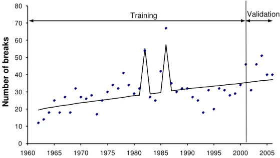
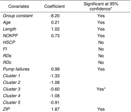
Example. The same dataset (from Calgary) used to examine the ranking models is used here to illustrate the application of the NHPP-based model. In addition, Calgary embarked on a (on-going) hotspot cathodic protection program in 1970. The model was trained on 40 years failure data from 1962 to 2001. The clustering scheme used was the same as illustrated in Figure 2. The coefficients obtained from training were used to forecast breaks for validation for years 2002-2006. The results are illustrated in Figures 4 and 5 and summarized in Tables 9 and 10. The following should be noted:

• The two outliers in 1982 and 1986 were likely the result of pumping station failures that occurred in these years causing a significant spike in the number of pipe failures. A user-defined time-dependent covariate (or time-series) was created to represent these events qualitatively (in this time series, a unity was assigned to years 1982 and 1986 and zeros to all other years). As expected, these outliers were captured by the trained model, likely resulting in more realistic values for the other covariates, especially the ageing rate. The assignment of unity to 1982 and 1986 in the time series implies that the impact of the pump failures was identical in those two years, which of course we have no way of knowing for sure. This example should not be viewed as over-fitting because it is based on relevant available data.

Figure 4. NHPP model example - training and validation (breaks aggregated by year)

Figure 5. NHPP model example - training and validation (breaks aggregated by pipe)

0 10 20 30 40 50 60 70 80 1960 1965 1970 1975 1980 1985 1990 1995 2000 2005 Training Validation N um ber o f br eaks 0 2 4 6 8 10 12 14 16 0 2 4 6 8 10 12 14 16

Observed breaks - training

M odel led br eaks Equality line

Over estimation zone

Under estimation zone

Observed breaks - validation 0 1 2 3 4 0 1 2 3 4

Table 9. Summary of NHPP model example results Covariates Coefficient Significant at 95%

confidence*

Group constant -8.20 Yes

Age 0.21 Yes Length 1.02 Yes NOKPF 0.73 Yes HSCP No FI No RDs No RDc No

Pump failures 0.99 Yes

Cluster 1 -1.33 Cluster 2 -1.08 Cluster 3 -0.60 Yes* Cluster 4 -1.08 Cluster 5 -0.91 ZIP 1.87 Yes

* The cluster covariates were tested for statistical significance as a block of 5 covariates, i.e., the likelihood ratio was compared to χ₅2 ≅11.07

Table 10. Ranking ability of NHPP model example results

n break(s) in validation period n = 1 n = 2 n = 3 n = 4 n = 5

# pipes with at least n (observed) break(s) out of 1091 pipes in group

170 30 6 2 0

# of pipes, k, identified correctly 61 8 1 1 n/a P-value (probability of identifying k

pipes by pure chance) 0.0 0.0 0.033 0.004

• The ageing covariate τ(t)=Ln(g_i,t)was used in this example. An examination of the coefficients (Table 9) reveals that background ageing was therefore proportional to the fifth root (power of about 0.2) of pipe age.

• Climate covariates as well as the hotspot CP (HSCP) covariate were found to be not

buried at a depth of 2.4 m, which may explain the insignificant impact of FI and RDs covariates.

• The positive sign of NOKPF may point to a “worse than old” condition (in repairable systems four repair-related conditions are observed, “good as new”, “good as old”, “better than old” and “worse than old”).

• The length covariate in this case study was taken as the Ln (natural log) of pipe length, which means that the number of estimated break was nearly linearly proportional to the length of the pipe (relatively strong dependency).

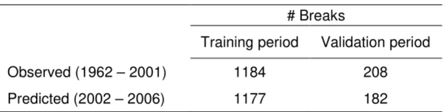
• While the NHPP-based model was quite accurate in predicting the total (cumulative) number of breaks that occurred between 2002 and 2006 (Table 11), it was not as successful in

estimating the number of breaks per pipe.

Table 11. Predicted vs. observed breaks (cumulative) # Breaks

Training period Validation period

Observed (1962 – 2001) 1184 208

Predicted (2002 – 2006) 1177 182

The NHPP model applied to this dataset tended to over-estimate the number of breaks for pipes that experienced few breaks, while under-estimate the number of breaks for those pipes that experienced a higher number of breaks. A similar tendency has been observed by others, e.g., Rostum (2000). The NHPP model predicts the expected number of break, which is a real

number, while the observed number of breaks is of course an integer. In this type of comparison it is expected that discrepancies between observed and predicted breaks would be relatively large, especially in individual pipes with few breaks. Moreover, this discrepancy may be even greater where there are many pipes with zero or few breaks and only a few pipes with many breaks.

Comparisons of models

As stated earlier, it is clear that the three ranking models and the NHPP-based model can only be compared on their ability to rank individual mains because only the latter model can actually forecast the expected number of breaks.

Data used for comparisons. Although datasets from several water utilities were made available

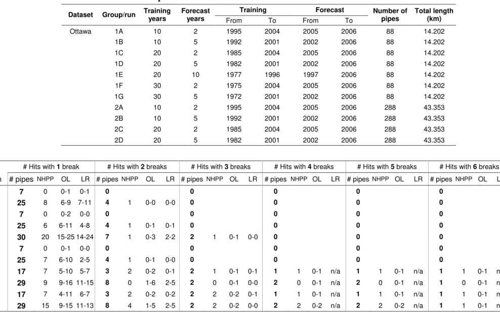
for this research, only datasets from Ottawa, Calgary and Scarborough (all in Canada) were used for the comparisons because of their relative historical depth. Two homogeneous pipe groups from each of the three utilities were selected at random for comparisons, for a total of six datasets. These pipe groups varied in vintage, diameter, material, and operational features. Each group was trained on various training periods with various combinations of covariates and various forecast periods for a total of 37 scenarios (runs), as detailed in Table 12. The

comparisons were done only on their ranking abilities for the validation period and not on the training results. Results of these comparisons are presented in Tables 13 through 15. It should be noted that in trial runs, the NBC (naïve Bayesian classification) model produced results that largely mimicked the results obtained from the LogReg (Logistic regression) model.

Consequently, the NBC-based model was not included in the comparison tables below. As noted earlier, the OL (Ordered lists) model (as well as the NBC model which was not included in the comparisons below) uses a search heuristic technique with random elements (genetic algorithm or GA) for training. Consequently, repetitions of an identical scenario can yield different results. In the comparisons, each scenario was repeated 16 times for the OL model. In the comparison tables, the results of the OL model are presented as range of minimum to maximum “hits” obtained from these multiple scenarios. The LogReg (Logistic regression) model does not use GA for training; however, as noted earlier, there are numerous potential covariates and many possible combinations for training the model. Different combinations of covariates yield different training and validation results for the same scenario. In the

comparisons, outcomes were determined from 16 different combinations (scenarios) of

covariates in the LogReg model. In the comparison tables, the results of the LogReg model are presented as range of minimum to maximum “hits” obtained from these multiple scenarios.

Table 12. Datasets and scenarios used for comparisons of models

Group City Material Diam. _(mm) Vintage Hotspot _CP Retrofit _{CP pipes} # of Length _(km) Training _(years) Forecast _(years)

1 Ottawa CI 150 1951-60 1990 Yes 88 14.20 10, 20, 30 2, 5, 10 2 Ottawa DI 150 1971-80 1990 No 288 43.35 10, 20 2, 5 3 Calgary CI 200 1961-65 1970 No 280 27.06 10, 20, 30 2, 5, 10 4 Calgary PDI 150 1971-75 1970 No 585 48.33 10, 20, 30 2, 5, 10 5 Scarb. AC 150 1951-60 - - 107 20.61 10, 20, 30 2, 5, 10 6 Scarb. DI 200 1966-75 1984 No 128 16.33 10, 20 2, 5