Publisher’s version / Version de l'éditeur:
CCWI 2013: 12th International Conference on Computing and Control for the
Water Industry, 2013-09-04
READ THESE TERMS AND CONDITIONS CAREFULLY BEFORE USING THIS WEBSITE. https://nrc-publications.canada.ca/eng/copyright
Vous avez des questions? Nous pouvons vous aider. Pour communiquer directement avec un auteur, consultez la première page de la revue dans laquelle son article a été publié afin de trouver ses coordonnées. Si vous n’arrivez pas à les repérer, communiquez avec nous à PublicationsArchive-ArchivesPublications@nrc-cnrc.gc.ca.
Questions? Contact the NRC Publications Archive team at
PublicationsArchive-ArchivesPublications@nrc-cnrc.gc.ca. If you wish to email the authors directly, please see the first page of the publication for their contact information.
NRC Publications Archive
Archives des publications du CNRC
This publication could be one of several versions: author’s original, accepted manuscript or the publisher’s version. / La version de cette publication peut être l’une des suivantes : la version prépublication de l’auteur, la version acceptée du manuscrit ou la version de l’éditeur.
Access and use of this website and the material on it are subject to the Terms and Conditions set forth at
Remaining life and economics of inspection in large-diameter pipelines
Kleiner, Yehuda
https://publications-cnrc.canada.ca/fra/droits
L’accès à ce site Web et l’utilisation de son contenu sont assujettis aux conditions présentées dans le site LISEZ CES CONDITIONS ATTENTIVEMENT AVANT D’UTILISER CE SITE WEB.
NRC Publications Record / Notice d'Archives des publications de CNRC:
https://nrc-publications.canada.ca/eng/view/object/?id=58677335-4d2a-4f1f-a77d-6bd3700d6085 https://publications-cnrc.canada.ca/fra/voir/objet/?id=58677335-4d2a-4f1f-a77d-6bd3700d6085Remaining life and economics of inspection in large-diameter
pipelines
Yehuda Kleiner
National Research Council of Canada, 1200 Montreal rd. Ottawa, ON. K1A 0R6, Canada
Abstract
A probabilistic approach is proposed, in which the economic life of a large-diameter buried pipe is expressed as a function of various factors, including the cost and efficiency of inspection. Expert knowledge is initially used to estimate the pipe expected remaining life as well as the impact of inspection technology on this estimate. As ‘hard’ data are obtained about the pipe, through actual recorded failures as well as through systematic and opportunistic inspection, these data are used to update and refine the initial estimates. The approach supports rational decisions, about pipe renewal timing, inspection scheduling ands size of investment in an inspection campaign.
Keywords: Large-diameter pipes, remaining life, inspection economics, probabilistic, asset management, decision-support
1. Introduction
As pipes deteriorate, their likelihood of failure increases. In small-diameter water distribution mains, where failure consequences are relatively low, a certain level of failure frequency can typically be tolerated. In contrast, failure consequences in large-diameter mains are typically high, leading to a preferred strategy of failure avoidance. Ideally, with perfect information about, and understanding of, deterioration and failure mechanisms, a pipe would be scheduled for renewal just before it is about to fail, thus avoiding failure while optimizing the use of renewal budgets. However in reality, with less than perfect knowledge, one can only estimate this ‘sweet spot’ of renewal timing.
Numerous approaches have been reported in the literature on modelling deterioration and making decisions on the renewal of buried pipes, though most address sewer mains (for which CCTV inspection data are more abundant) rather than trunk water mains. Markov process-based approaches include Abraham and Wirahadikusumah (1999), Kathula and McKim (1999), Jiang et al. (2000), Kleiner (2001), Micevski et al. (2002), Baik et al. (2006) and others. Logistic regression-based approaches include Ariaratnam et al. (2001), Davies et al. (2001), Cooper et al. (2000) and others. Soft-computing approaches include artificial neural networks, e.g., Tran et al. (2009); fuzzy computing methods, e.g., Kleiner et al. (2006a, b), Rajani et al. (2006) and others. Other noteworthy approaches include Bayesian belief networks by Hahn et al (2002), Younis and Knight (2010) with an ordinal regression-based model and dynamic programming by Ugarelli and Di Federico (2010).
Evidence about the condition of the pipe as well as plausible failure mode is provided through observable or measurable signs (or distress indicators) as well as through inferential indicators (such as soil properties, environmental or operation conditions) that point to the potential existence of deterioration mechanisms. The role of asset inspection is to observe and document the existence and extent of distress indicators. However, inspection carries its own cost, as well as accuracy limitations, it should therefore be undertaken judiciously and its benefits should be weighed against its cost.
The approach proposed here is probabilistic, where pipe-end-of-life is defined as an economic outcome of the trade-off between the expected cost of pipe deterioration and the cost of its renewal. Pipe inspection is an important factor that influences the expected failure cost of deteriorating pipes and the proposed approach takes this influence into consideration. This enables to determine what level of investment in pipe inspection is economically justified.
Expert knowledge is initially used to estimate the expected remaining life of a large-diameter pipe, as well as the impact of inspection technology on this estimate. As ‘hard’ data are obtained about the pipe, through actual recorded failures as well as through systematic and/or opportunistic inspection, these data are used to update and refine the initial estimates.
A case study is presented to demonstrate the approach and its performance and applicability. This approach can be an attractive proposition for the effective management of large-diameter pipe assets, leading to rational decisions
about when to plan the pipe renewal, or alternatively when to schedule the next inspection. The approach also provides a rational assessment about the size of investment in an inspection campaign that can be economically justified at the various stages in the pipe life. It also delineates the pipe age at which pipe owner should undertake regular pipe inspection.
2. Definitions
To establish the theoretical basis for the approach, the following definitions are made:
Pipe – a relatively homogeneous pipe section of length L, comprising pipe segments of length l each (a total of n = L/l segments in a pipe). All segments of a pipe are considered to belong to the same (statistical) population. Pipe segment – a basic component of a pipe. For practical reasons it is convenient to define it as a single
bell-to-spigot unit in the case of jointed pipe.
Pipe failure – occurs when a single segment fails, resulting in segment replacement or significant renovation, which makes the segment good as new. Pipe failure is associated with cost of failure, which includes direct, indirect and social costs.
Pipe imminent failure – when inspection determines that a single pipe segment is deteriorated to a degree that failure can occur at any moment, and almost certain to occur before next inspection. In the following time-to-failure analysis pipe time-to-failure and pipe imminent time-to-failure are considered to be equivalent events, i.e., ‘time to time-to-failure’ and ‘time to imminent failure’ are equivalent.
Pipe rehabilitation (unscheduled) – upon failure, the segment can be rehabilitated/replaced. It is assumed that the rehabilitated segment is as good as new (since the segment is exposed for repair the measure needed to make it good as new is easily determined).
Pipe rehabilitation (scheduled) – undertaken following inspection, upon discovery of a substantial deficiency or imminent failure. Here too it is assumed that the rehabilitated /replaced segment is as good as new.
Pipe minor repair – whereas rehabilitation makes the pipe good as new, minor repair restores the pipe to as good as old. Examples: small leaks repaired with clamps, joint leak repaired with re-caulking, etc. When several minor repairs on a single segment lead to its replacement, it is considered a failure.
Probability of detection (POD) – as no inspection technology is perfect, there is some likelihood that a substantial deficiency will not be detected.
Probability of false positive (PFP) – probability that an inspection will erroneously identify a substantial deficiency.
Pipe end of life – when it is no longer economical to perform scheduled and unscheduled local rehabilitation (including segment replacement) while carrying the risk of failure of segments that have not been
replaced/renovated. In other words, the expected cost of catastrophic failures plus expected cost of imminent failure pre-emption become higher than the cost to replace (or renovate) the entire pipe
3. Time to failure of a pipe segment
The time to failure of a pipe segment is assumed to follow some probability distribution. The vast majority of pipe owners will have insufficient data to ascertain with any accuracy the exact type of distribution. Consequently, the Weibull distribution is proposed because of its relative simplicity and the fact that it is widely used to model component time to failure; however, it must be noted that the approach outlined here can be applied with any probability distribution that is found suitable. Ideally, the estimation of parameters for the probability distribution would be done based on actual historical data of failures or imminent failures in the pipe. However, as stated above, data about segment longevity are often lacking or not available, therefore a simple method to estimate parameters, based on expert opinion is also provided. The 3-parameter Weibull probability is
1
1 x x x F x e f x e
(1)where F(x) is the cumulative density function (cdf), f(x) is the probability density function (pdf), is the scale parameter and is the shape parameter and γ is the offset parameter. In the context of time to failure analysis, parameter γ represents a period since installation, during which no failures are expected (in some publications such a parameter is termed “period of resistance” to failure and is also linked to a warrantee period, where any failure is the responsibility of the contractor). Consequently, parameter γ can usually be estimated directly by utility experts. Parameters and can subsequently be computed based on two known pairs x1, F(x1) and x2, F(x2), using Eqs. (2):
1 2 1 2 1 1 1 ln ln 1 ln ln 1 ln ln ln 1 F x F x x x x F x
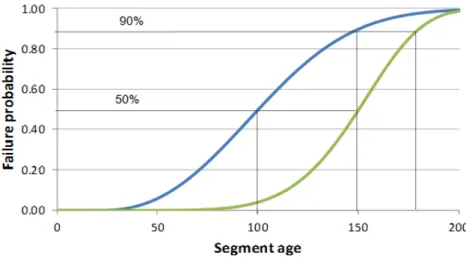
(2)For example, suppose that utility experts can agree that they believe that for a certain pipe no segment will fail in the first 20 years after installation. Suppose that they can further agree that the median life (i.e., the time since installation during which 50% of the population will not fail) of segments is 100 years and 10% will survive with no failure to 150 years, then parameter γ = 20 years and equation (2) can be used to obtain parameters = 92.8 and
=2.47. Fig. 1 illustrates the resulting probability distribution of age at failure. Another example with a more (right) skewed distribution is provided in Fig. 1, where the same γ = 20 is considered and 50% of the pipe segments are believed to survive (without failure) to the age 150 years, and 10% to 180 years (= 138.5 and = 5.78). As can be seen, the Weibull distribution is quite flexible and can represent a wide array of shapes.
Fig. 1. Examples probability distribution of pipe segment time to failure.
These expert opinion-based initial estimated parameters are referred to as ‘semi-informative’ parameters because they are not (or are minimally) based on ‘hard’ failure data. A detailed description of how to continually update these semi-informative parameters using real incoming failure and inspection data is provided in a later section.
4. Pipe rate of failure
We define failure rate (t) as the expected annual number of failures or imminent failure in year t:
1
1 t tt
n F t
F t
n e
e
(3)where n is the number of segments in the pipe.
5. Pipe life-cycle cost
5.1. Cost of single cycle
Let Crdenote entire pipe replacement cost, Cfdenote segment failure cost (including emergency repair and all direct, indirect and social costs) and Cbdenote the cost of planned segment rehabilitation/replacement (i.e., cost of failure pre-emption). For simplicity, it is tentatively assumed that the cost of inspection can be somehow expressed in terms of annual disbursements, CI. The expected total annual cost associated with the pipe at year t is given by
b
1
f b IC t
t POD C
POD C
nPFP C
C
(4)In the life-cycle of the pipe, we assume that as the pipe ages and deteriorates C(t) increases over time until the pipe is replaced at its end of life tend. In reality, a relatively small fraction of the n segments will have been renewed by tend, therefore it is reasonable to assume for simplicity that a single segment will not fail more than once during one pipe renewal cycle (i.e., a renewed/replaced segment is assumed to survive to tend).
The total discounted cost of a complete renewal cycle excluding initial installation cost but including pipe replacement cost at year T, is given by (r is the social discount rate)
11
1
1
T b f b I r cycle t t tt POD C
POD C
nPFP C
C
C
C
r
r
(5)5.2. Cost of perpetual cycles to infinity
The life-cycle of the pipe will theoretically include perpetual renewal cycles to infinity. The consideration of perpetual renewal cycles obviates the need to define a planning horizon and consider the residual value of the pipe at the end of this planning horizon. If as a first approximation we assume that these perpetual renewal cycles are identical, it can be shown that the present value of the cost of the infinite series of renewal cycles is given by
inf1
1
1
T cycle Tr
C
T
C
r
(6)The value T = T** that minimises C
inf is the expected useful life of the pipe, given the aforementioned assumptions. The value of T**can easily be found by using trial and error or simple numerical techniques, such as the ‘Solver’ utility in MS-Excel.
5.3. Life-cycle cost of existing pipe (present to next replacement) and remaining useful life
Suppose we want to analyse an existing pipe of age to, with segment time-to-failure distribution parameters, and γ; cost of replacement Cr, cost of failure Cfand cost of failure pre-emption Cb. The failure rate of this pipe (t) is computed with equation (3) The total life-cycle cost Ctotof this pipe from present to infinity is given by
** 0 11
1
1
T r r b f b I tot t T tC
C T
t
t POD C
POD C
nPFP C
C
C
T
r
r
(7)The value T = T*that minimises C
totis the expected remaining useful life of the pipe, given the aforementioned assumptions. The value of T*can easily be found by using trial and error or simple numerical techniques, such as the ‘Solver’ utility in MS-Excel.
5.4. When should a pipe owner start undertaking regular inspection?
It is intuitively understood that inspection is justified only when its benefits outweigh its cost. From Eq. (5) it can be seen that the net benefits (NB) of inspection at year t are given by
f
b
1
f b I
NB t
t C
t POD C
POD C
nPFP C
C
(8) where the left term on the right hand side is the ‘do nothing’ expected cost and the secont term (in the curly braces) is the annual expected cost including inspection. Rearranging Eq. Error! Reference source not found.8) we obtained that the year t = Tiat which the benefits of inspection equal its cost (i.e., NB = 0) is when
I
b
i f bC
nPFP C
t T
POD C
C
(9)where the numerator represents inspection costs (false positives are an un-intended cost) and the denominator represents benefits. Since the rate of failure is non-decreases with pipe age it makes economic sense to avoid inspection in the early years of the pipe when t ≤ Ti.
6. Influence of inspection technology on pipe life-cycle cost and remaining life
Eq. (7) can be readily used to quantify the impact of an inspection technology on the pipe life cycle cost (Ctot) and on its remaining life (t*). Essentially, as the pipe deteriorates the expected number of imminent failure increases. Inspection allows to pre-empt some of these imminent failure (through scheduled repair), thus preventing them from ‘maturing’ into a full blown failure, which typically carries a higher cost than scheduled repair. The higher the POD of a given inspection technology the higher the expected cost savings, which in turn justifies a higher investment in this technology. This concept is intuitively understood by all practitioners and the proposed approach allows quantifying it in a rational manner.
Example:
Assume a (to.=) 30-year old pipe, 800m long (n = 200 segments, 4m long each).
The probability distribution in the previous example (left curve in Figure 1) is assumed to govern segment time-to-failure, with = 93, = 2.5 and γ = 20 years.
Replacement cost is estimated at Cr= $800,000, cost of failure Cf= $100,000/event and cost of planned repair
Cb= $20,000/event.
Future replacement pipes are assumed to have superior longevity, with time-to-failure distribution parameters corresponding to the right curve in Figure 1, i.e., ’ = 138.5, ’ = 5.78 and γ’ = 20 years.
Costs associated with the replacement pipes are assumed to be identical to the existing pipe, i.e., at Cr= C’r,
Cf= C’f and Cb= C’b.
Assume that for both current and future pipes inspection of the entire pipe costs $50,000, with POD = 0.5 and
PFP = 0, and that this inspection provides a 5-year reliable identification capability (i.e., there is no need to
inspect more frequently than every 5 years. Consequently, the annual inspection cost can be approximated at
CI= $10,000.
Using equations (3) through (6), the steady-state future cycle duration is calculated to be T**= 95 years. The present value (discounted to the next replacement year) of the perpetual cost to infinity of all future replacement cycles (including O&M and capital investment but excluding the capital investment in the next replacement) is calculated to be Cinf(T**) = $416,000.
Using equation (7), the optimal time to replace the existing pipe (i.e., its remaining useful life) is computed to be
T*= 8 years. The total cost (discounted to the present) from the present to infinity is computed to be C tot(T*) = $1,160,000.
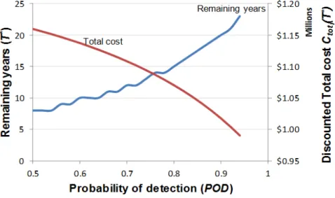
Clearly, a higher inspection POD will ‘convert’ actual failures to pre-empted failure, thus reducing total cost and extending the useful life of the current pipe. Figure 2 illustrates the effect of POD on the pipe remaining life and total
life-cycle cost. It shows that in our example increasing POD from 0.5 to 0.9 for example, can extend the remaining economic life of the current pipe from 9 to 20 years and reduce the discounted life cycle cost from about $1.16M to about 1.0M. This would justify increasing the annual inspection budget by up to (1.16M - 1.0M) / (20 - 8) ≈ $12K. If we continue to assume that inspection will be implemented at 5-year intervals, this means that an inspection up-front cost of up to approximately $110K can be justified.
Figure 3 illustrates how life-cycle costs and remaining life vary at different pipe ages. Figure 3a shows that improved POD will reduce the expected life-cycle costs at any pipe age. However, the pipe expected useful (economic) life varies depending on POD level. As the pipe reaches its maximum useful life it is assumed to be replaced shortly and therefore the marginal benefit of inspection declines (curves become closer to each other).
Figure 3b demonstrates that as long as the pipe is not older than a certain threshold, its age has no bearing on the remaining life for a given POD. In our example, at age 20 the pipe remaining life with POD = 0.8 is 25 years for a total of (20 + 25 =) 45 years of useful economic life. Similarly, at age 30 with the same POD, remaining life will be 15 years, for a total useful economic life of 45 years, and so forth (total useful life always adds up to 45 years). However, at age 40 a POD of at least 0.7 would be needed to extend the pipe economic remaining life.
Fig. 2. Impact of POD on remaining life and total cost.
7. Using historical data to estimate/update distribution parameters
There are three types of historical data that can be used to estimate the parameters of the probability distribution of time to failure of the population of segments in a pipe. These include actual failures, imminent failure observed at an inspection session (from a statistical point of view imminent failures are treated here as failures) and not-yet-failed (surviving) segments at the analysis period.
While the date of an actual failure provides an actual data point, imminent failures observed at an inspection session can only be associated with a time interval (e.g., since last inspection or since installation) because the exact timing at which they reached imminent failure state is not known. Such failures (or imminent failures) that are known to have occurred within a time interval are termed ‘interval-censored data’. The pipe segments that are known to have survived to the end of the observation period (in our case the present analysis timing) are termed ‘right-censored data’.
In some cases it is possible that the data are so-called left-truncated, i.e., the pipe owner/operator started recording failures only after a certain date, resulting in a ‘blank’ period between pipe-installation and that date, during which failures may or may not have occurred. In the analysis presented here no special consideration is given to left truncated data and the entire period between pipe-installation and first inspection is considered as interval-censored data regardless of when record keeping began.
The maximum a posteriori (MAP) method is proposed for estimating distribution parameters. This method is a derivative of the Bayesian approach to estimate distribution parameters, based on some prior knowledge (or belief) combined with observational data. This approach is especially useful in cases where observational data are scarce (as is the case in most large-diameter buried pipelines) but there exists some general knowledge about the behaviour of the population at hand, typically elicited from experts.
We assume that our Weibull distribution parameters , , are normally distributed with means , , and
standard deviations , , respectively. The log-likelihood of the posterior function is given by
1 2 2 2 2 2 2 1 1 1ln
ln
2
2
2
1
ln
ln
ln
; , ,
j j R R i i K j i jR
R
t
t
M
T
m
e
e
t T
(10)where R is the total number of recorded actual failures, tiis the pipe age at failure i (i = 1, 2,..,R), M is the number of surviving segments at the year of analysis and T is the pipe age at the year of analysis, K is the number of inspections ever undertaken on a given pipe. Inspection j is undertaken at pipe age τj(j = 0, 1, 2, ...,K). Note that τj=0 refers to the time of γ years after pipe installation (before then the pipe is expected to have zero failures) and therefore τj=0= γ. mjdenotes the number of imminent failures discovered at inspection j (it is consistently assumed that mj=0= 0). The maximum a posteriori (MAP) estimates , , are those values of parameters α, β and γ which maximize the value of the posterior probability in Eq. (10).
8. Concluding comments
A probabilistic approach was presented, where pipe-end-of-life is defined as an economic outcome of the trade-off between the cost of pipe deterioration and cost of its renewal. The pipe end of life is when the expected cost of catastrophic failures plus expected cost of planned repairs/renewal become higher than the cost to replace (or renovate) the entire pipe The proposed approach takes into consideration the influence of pipe inspection on the cost of deterioration and, which enables the determination of an economically justified level of investment in pipe inspection.
Expert knowledge is initially used to estimate the pipe expected remaining life. As ‘hard’ data are obtained about the pipe, through actual recorded failures as well as through systematic and opportunistic inspection, these data are used to update and refine the initial estimates, using a Bayesian updating technique.
The probability of detection POD refers to the overall capability of an inspection technology coupled with the interpretation of the inspection results to obtain accurate information about the pipe condition. In reality, it is not easy to determine with accuracy the POD of a given inspection technique or NDE (non-destructive evaluation) technology. Many NDE technologies are proprietary and data about their POD and PFP are either nonexistent or not publicly available. Estimation of POD must be done in consultation with experienced personnel as well as with the technology vendor, if applicable.
Often, the interpretation of inspection results will be coded as some ordinal condition rating, such as condition 1 to 5 or 1 to 7, etc., with or without linguistic descriptors such as Good, Fair, Bad, etc. To use the model presented here it is necessary to determine a threshold rating, at which a pipe section will be considered to be in a state of imminent failure. For example, if the pipe condition is rated on a scale of 1 (best) to 7 (worst), the practitioner may decide that a condition rating of 6 or higher is considered ‘imminent failure’.
An additional benefit of inspection is the possible avoidance of grossly premature replacement. However, this benefit cannot be adequately quantified without knowing the basis upon which an untimely replacement was undertaken.
Acknowledgement
The research reported in this paper was co-sponsored by the Water Research Foundation (WaterRF), the National Research Council of Canada (NRC) and in-kind support of water utilities from the United States and Canada.
References
Abraham, D.M., Wirahadikusumah, R., 1999. Development of prediction model for sewer deterioration, In: Proceedings of the 8th Conference Durability of Building Materials and Components, M.A. Lacasse and D.J. Vanier (Eds.), IRC, NRC, pp. 1257-1267, Vancouver.
Ariaratnam, S.T., El-Assaly, A., Yang, Y., 2001. Assessment of infrastructure needs using logistic models, ASCE Journal of Infrastructure Systems, 7(4), 160-165.
Baik, H.S., Jeong, H.S., Abraham, D.M., 2006. Estimating transition probabilities in Markov chain-based deterioration models for management of wastewater systems. J. of Water Resources Planning and Management, 132(1), 15–24.
Cooper, N.R., Blakey, G., Sherwin, C., Ta, T., Whiter, J.T., Woodward, C.A., 2000. The use if GIS to develop a probability-based trunk mains burst risk model, Urban Water, 2, 97-103.
Davies, J.P., Clarke, B.A., Whiter, J.T., Cunningham, R.J., Leidi, A., 2001. The structural condition of rigid sewer pipes: a statistical investigation, Urban Water, 3, 277-286.
Hahn, M.A., Palmer, R.N., Merrill, M.S., Lukas, A.B., 2002. Expert system for prioritizing the inspection of sewers: knowledge base formulation and evaluation, Journal of Water Resources Planning and Management, 128(4), 121-129.
Jiang, M., Corotis, R.B., Ellis, J.H., 2000. Optimal life-cycle costing with partial observability, Journal of Infrastructure Systems, 6(2), 56-66. Kathula, V.S., McKim, R., 1999. Sewer deterioration prediction. In: Proceedings Infra 99 International Convention, CERIU, Montreal, Nov. Kleiner, Y., 2001. Scheduling inspection and renewal of large infrastructure assets, Journal of Infrastructure Systems, 7(4), 136-143.
Kleiner, Y., Sadiq, R., Rajani, B.B., 2006a. Modelling the deterioration of buried infrastructure as a fuzzy Markov process. Journal of Water Supply Research and Technology: Aqua, 55, (2), 67-80.
Kleiner, Y., Rajani, B.B., Sadiq, R., 2006b. Failure risk management of buried infrastructure using fuzzy-based techniques. Journal of Water Supply Research and Technology: Aqua, 55, (2), 81-94.
Micevski, T., Kuczera, G., Coombes, P., 2002. Markov model for storm water pipe deterioration. Journal of Infrastructure Systems, 8(2), 49-56. Rajani, B.B., Kleiner, Y., Sadiq, R., 2006. Translation of pipe inspection results into condition rating using fuzzy synthetic valuation technique.
Journal of Water Supply Research and Technology: Aqua, 55, (1), 11-24.
Tran, H. D., Perera, B.J.C., Ng, A.W.M., 2009. Predicting Structural Deterioration Condition of Individual Storm-Water Pipes Using Probabilistic Neural Networks and Multiple Logistic Regression Models”, J. of Water Resources Planning and Manag., 135(6), 553-557. Ugarelli, R., Di Federico, V., 2010. Optimal scheduling of replacement and rehabilitation in wastewater pipeline networks. J. of Water Resources
Planning and Management, 136(3), 348-356.
Younis, R., Knight, M.A., 2010. A probability model for investigating the trend of structural deterioration of wastewater pipelines, J. Tunnelling and Underground Space Technology 25, 670–680.