Batch Bayesian optimization

Batch Bayesian Optimization

by

Nathan Hunt

Submitted to the Department of Electrical Engineering and Computer

Science

in partial fulfillment of the requirements for the degree of

Master of Science

at the

MASSACHUSETTS INSTITUTE OF TECHNOLOGY

February 2020

©

Massachusetts Institute of Technology 2020. All rights reserved.

Signature redacted

Author.

...

Department of Electrical Engineering and Computer Science

Ja ry 10, 2020

Signature redacted

Certified by...

David K. Gifford

Professor of Electrical Engineering and Computer Science

Thesis Supervisor

A ccepted by ...

MASSACHUSETS INSTITUTE OFTECHNOLOGY

MAR 13 2020

LIBRARIES

Professor of Electrical

Signature redacted

Llslie4 (*olodziejski

Engineering and Computer Science

MITLibraries

77 Massachusetts Avenue

Cambridge, MA 02139 http://Iibraries.mit.edu/ask

DISCLAIMER NOTICE

Due to the condition of the original material, there are unavoidable

flaws in this reproduction. We have made every effort possible to

provide you with the best copy available.

Thank you.

Pages contain copy print steak marks.

Batch Bayesian Optimization

by

Nathan Hunt

Submitted to the Department of Electrical Engineering and Computer Science on January 10, 2020, in partial fulfillment of the

requirements for the degree of Master of Science

Abstract

Bayesian optimization is a useful technique for maximizing expensive, unknown func-tions that employs an acquisition function to determine what unseen input point to query next. In many real-world applications, batches of input points can be queried simultaneously for only a small marginal cost compared to querying a single point. Most classical acquisition functions cannot be used for batch acquisition, and thus batch acquisition strategies are required. Several such strategies have been developed in the past decade. We review and compare batch acquisition strategies in a variety of settings to assist practitioners in selecting appropriate batch acquisition functions and facilitate further research in this area.

Thesis Supervisor: David K. Gifford

Acknowledgments

As I began graduate school, I expected it to be easier in some ways than my un-dergraduate education. However, I soon found being a graduate student to be much more taxing as I immediately dealt with the need to find funding to even be able to

continue. After this was resolved, I struggled to find good research questions and at

times felt demoralized when even approaches I had had hope for failed to yield useful

results. I'm thus all the more grateful for the support that I've received during these

years.

I am greatly indebted to my advisor, Dave Gifford, for the financial, academic, and moral support that he's given me throughout this work. Though the most stressful

time of my week was often when I was preparing to meet with him, and worried about

the slow or nonexistent progress I had made since the last week, Dave always showed

great patience, never demeaned my work, and provided useful discussions on what

to do next. I'm very grateful that he made finishing this thesis possible. I'm also

grateful for the other members of the Gifford lab who I've been able to work with, especially Sid Jain for his help developing new Bayesian optimization methods.

I'm also thankful to Marzyeh Ghassemi and Pete Szolovits for their mentoring

in my research during my last year of undergrad. In Pete's group, I felt like a real

researcher, not just an undergrad. Marzyeh's persistent optimism raised my spirits

through many setbacks, and she convinced me that I could do real research worth

sharing. I doubt I would have made it into grad school without their support. I greatly

appreciate the interactions I was able to have with the other members of Pete's group

as well, especially Harini Suresh, Tristan Naumann, and Matthew McDermott.

I'm grateful for my siblings, mother, and other family members for their support

during these years and for sharing their lives with me. I'm also grateful for my friends, especially for reminding me how much there is to life outside of earning degrees.

I am especially grateful for my wife, Rachel Mok, and our children Sammy and

Grace. I'm thankful I can come home to hugs, singing, reading stories, building, and being the voice of every stuffed animal, for how they bring me back to the

greater purpose of my life. I appreciate that Rachel listens, at least most of the time, when I want to talk about papers, algorithms, code, and what shapes have infinite

symmetries. I'm grateful for her patience with the imperfect partner that I am and

the journey that we undertake together. I'm thankful that she believes in my dreams, sometimes more than I do, and sacrifices so we might achieve them. The love, time, and effort that she devotes to our family is one of my greatest blessings.

Finally, I owe a debt of gratitude for the divine assistance that has carried me

Contents

1 Introduction 1.1 R elated W ork . . . . 2 Background 2.1 Notation ... ... ... ... . 2.2 M odels . . . . 2.2.1 Gaussian Processes . 2.2.2 Other Models . . . .

2.3 Sequential Acquisition Functions. 2.3.1 Probability of Improvement 2.3.2 Expected Improvement . . 2.3.3 Upper Confidence Bound.

2.3.4 Thompson Sampling .

2.3.5 Other . . . .

3 Batch Acquisition Functions

3.1 q-points Expected Improvement (qEI) . . . .

3.1.1 Kriging Believer (KB) . . . .

3.1.2 Con tant Liar (CL) . . . . 3.2 Local Penalization (LP) . . . . 3.3 Thompson Sampling . . . . 3.4 Batch Upper Confidence Bound (BUCB) . . . .

3.5 Upper Confidence Bound with Pure Exploration

15 16 19 20 21 22 24 26 26 27 27 28 28 31 32 33 33 34 36 37 38 (UCB-PE)

3.6 Distance Exploration (DE) . . . . 3.7 Budgeted Batch Bayesian Optimization (B30) . . 3.8 k-means Batch Bayesian Optimization (KMBBO) 4 Experiments

4.1 Objective Functions . . . . 4.1.1 Test Functions . . . . 4.1.2 Dataset Maximization Tasks . . . . 4.1.3 Simulations . . . . 4.2 B aselines . . . . 4.3 Implementation Details . . . . 4.4 M etrics . . . .

5 Results

5.1 Low-dimensional, Continuous Objectives . . . . 5.2 Dataset Maximization Objectives . . . . 5.3 High-dimensional, Continuous Objectives . . . .

6 Conclusion A Test Functions B Extended Results

. . . .

. . . .

. . . .

38 40 41 43 43 43 43 45 45 46 47 49 51 51 53 55 57 63

List of Figures

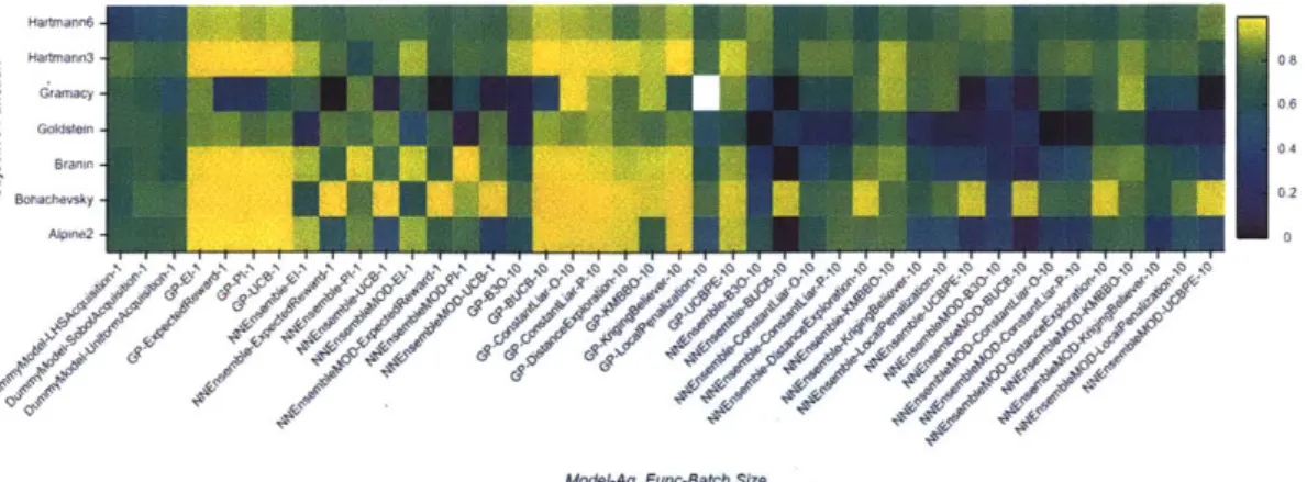
5-1 Median average gap metric for synthetic objective functions.... 5-2 Median average gap metric for discrete objective functions. . . . . . 5-3 Median average gap metric for high-dimensional objective functions. A-I The Gramacy function. . . . . A-2 The Branin function. . . . .

A-3 The Alpine2 function. . . . .

A-4 The Bohachevsky function. . . . .

A-5 The Goldstein function. . . . .

B-i Abalone ... B-2 Alpine2 ... B-3 Bohachevsky . B-4 Branin . . . . B-5 DNA Binding: B-6 DNA Binding: B-7 DNA Binding: B-8 DNA Binding: B-9 DNA Binding: B-10 Goldstein . . B-11 Gramacy ... B-12 Hartmann3 B-13 Hartmann6 B-14 Robot Push 52 52 53 59 59 60 60 61 64 64 65 65 66 66 67 67 68 68 69 69 70 70

. . . .

. . . .

. . . .

. . . .

ARX ...

BCL6 ...

CRX . . . .

EGR2 ... ESXi ...

. . . .

. . . .

. . . .

. . . .

List of Tables

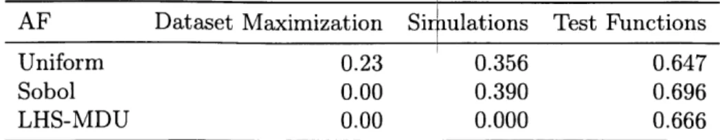
4.1 Overview of the objective functions. xi denotes the i-th dimension of the input point x. Some of these functions have been negated so that they are maximization problems when traditionally they would be minimizations. Alpine2 is defined for any number of dimensions, but we use it in 2 dimensions. Formulas that are excessively long are deferred to the appendix. . . . . 44 5.1 Gap metric performance of random baselines averaged over all

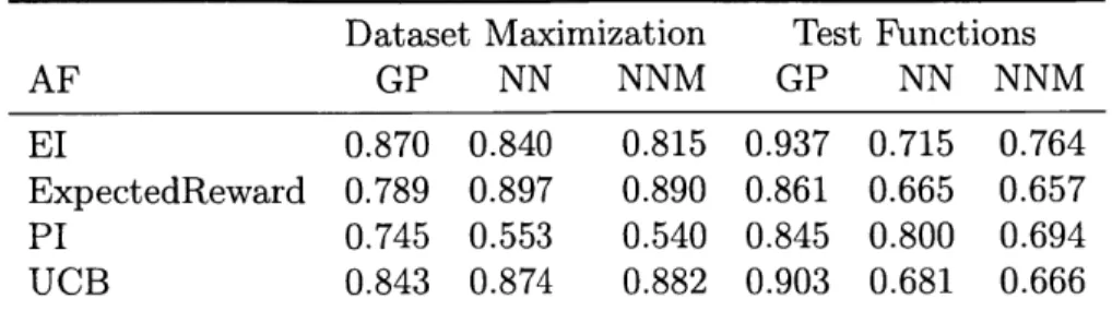
objec-tive functions of each class. AF = acquisition function. . . . . 49 5.2 Gap metric performance of sequential acquisition functions averaged

over all objective functions of each class. AF = acquisition function,

NN = neural network ensemble, NNM = neural network ensemble with

maximizing overall diversity method. . . . . 50 5.3 Gap metric performance of batch acquisition functions averaged over

all objective functions of each class. AF = acquisition function, NN = neural network ensemble, NNM = neural network ensemble with maximizing overall diversity method. . . . . 50

List of Algorithms

1 Bayesian Optimization . . . . 20 2 Kriging Believer . . . . 34 3 Constant Liar . . . . 35 4 Local Penalization . . . . 36 5 Thompson Sampling . . . . 37

6 Upper Confidence Bound with Pure Exploration . . . . 39

7 Distance Exploration . . . . 40

8 Budgeted Batch Bayesian Optimization . . . . 41

Chapter 1

Introduction

Most research in Bayesian optimization has been in the sequential setting where

the objective function is queried at a single point at a time. While this work has

been useful for many applications, there are also many domains where functions of

interest cannot reasonably be optimized sequentially. Instead, batches of points need

to be queried at once. Most sequential Bayesian optimization techniques are not

directly applicable in the batch setting. However, research interest in batch Bayesian

optimization has grown recently, and many batch acquisition functions having been

proposed in the past decade. However, not all of these have been compared with

each other. Here we introduce and compare all major batch Bayesian optimization

acquisition functions. In Bayesian optimization in particular, because the functions to

be optimized are expensive to evaluate, a practitioner is likely unable to try multiple

acquisition functions to determine which is best for their task. A review is thus useful

both to those hoping to apply batch Bayesian optimization in their work as well as

to facilitate further research.

Our contributions are as follows:

1. We describe many of the existing acquisition functions for batch Bayesian opti-mization. Having this information in one source is especially useful for

compar-ing the different strategies used for batch Bayesian optimization and considercompar-ing

next.

2. We test several batch acquisition functions on a variety of tasks and discuss their relative performance to help understand when certain functions will be

most useful.

3. We provide a modular, extensible software package which implements the ac-quisition functions used in our experiments.

In chapter 2 we discuss existing summaries of Bayesian optimization and highlight the contributions of this review. Chapter 3 provides an introduction to Bayesian op-timization including defining notation, describing the Gaussian process and other models, and presents multiple sequential acquisition functions. Chapter 4 reviews the batch acquisition functions studied in this work. Chapter 5 describes the ex-periments conducted including the various objective functions and implementation details. Chapter 6 showcases and discusses the results of these experiments. Chap-ter 7 concludes, summarizing the findings of this work and suggests areas for future research in batch acquisition functions.

1.1

Related Work

Three well-known reviews of Bayesian optimization optimization have already been written in the past couple of decades. [291 examined existing Bayesian optimization approaches including analysis of their strengths and weaknesses by applying them to one- and two-dimensional test functions. [4] reviewed a few sequential acquisition functions, showcased a couple of applications of Bayesian optimization, and provided general advice for practitioners. They mention briefly that work ir batch Bayesian optimization has begun. [46] review several sequential acquisition functions, including more recent ones such as entropy search[], GP-hedge[], and entropy search portfolio[]. They also discuss practical considerations in Bayesian optimization such as approxi-mation methods for Gaussian processes and methods of optimizing utility functions. Batch Bayesian optimization receives a subsection in this paper where the constant

liar and Kriging believer strategies, which will be explained later, are described and a few other approaches are mentioned by reference. Any of these papers, and especially the latest one, can be consulted for a more in-depth review of sequential Bayesian optimization. This review sets itself apart by focusing specifically on batch Bayesian optimization, especially the acquisition functions necessary for this.

[44] provide a review of probabilistic models, most involving neural networks, for contextual bandit problems. They exclusively use the Thompson sampling acquisition function, which can be used in a sequential or batch setting. These methods could be applied to Bayesian optimization tasks as well. In order to look more fully at different acquisition functions, we restrict ourselves to just three models: exact Gaussian pro-cesses, one approximation method for Gaussian propro-cesses, and one model involving neural networks.

Chapter 2

Background

The field of Bayesian optimization is concerned with finding an optimum (which

we will always call a maximum; any minimization problem can easily be converted

to a maximization problem through negation) of a function

f

which has no known analytic form or gradients and is costly to evaluate. For example,

f

may represent a physical or biological system where no model exists. As such, the learning of a

model for

f

should be optimized in as few evaluations as possible. Additionally, observations of

f

may be noisy. These constraints preclude traditional optimization techniques. Bayesian optimization approaches this task by learning a distribution

over functions based on previously observed data and using this to determine which

points to query

f

at next. This decision must balance exploration (querying points with higher uncertainty) and exploitation (querying points that are expected to have

high values). There are two main co nponents to a Bayesian optimization method: a

model, which determines the family f distributions over functions, and an acquisition

function, which determines how new query points are selected. A general algorithm

for Bayesian optimization is given in Algorithm 1. After describing notation, we

will discuss specific models, including what creating and updating them entails, and

Algorithm 1: Bayesian Optimization Input:

f:

function to be optimized

T: number of iterations

D: initial dataset

{(Xi,

yi),. . ., (X, Yn)} model = createmodel(D) for t in 1, ... , T : x = acquisitionfunction(model, D) y

f(x)

model.update(x, _y) D = D U

{(x,

y)}

return

argmax EX model.expectedvalue(x)

2.1

Notation

In order to discuss Bayesian optimization in greater detail, we establish the following notation.

"

f

is the objective function. Noise may be added to observations of it (see below). " X: the input space of

f.

The output space is R, or some subset thereof, so

that

f

: X -+ R. X is usually a box-constrained subset of Rd where d is the

dimensionality of X.

" y - f(x)

+

E: observations of f at x take this form, where c is noise that, generally, is assumed to be zero-mean and independent of x. We make these assumptions as well, so E [f(x)

+

E] = f(x). The most common case in the

literature is that E is normally distributed. " x* = argmaxXGX f(x) is the optimal point.

• y* = E [f(x*)

+

E] = f(x*) is the value of the optimal point.

• D = {(xi, y, .... , (x, y,)} is the previously observed dataset. T is is

popu-lated with new data points as they are acquired. We will also sometimes use X ={xi,..., x} and Y = {yi,..., yn}.

• f = p(f

I

D) is the current distribution over functions. Note that this involves

the particular input location x. Bayesian optimization seeks to improve f as an

approximation of

f

by choosing the best input points at which to observe

f.

L p(x), U(x) are the mean and variance, respectively, of f(x).

• x* = argmaxxcx E [f(x)] is the expected location of x* under f.

Sy* = E [f(x*)] is the expected value of x.

Sa(f , X) is an acquisition function which selects a point x c X to query f at next. Acquisition functions are often written as az(x) in the literature and the

acquired point is then argmaxXEX a(x). Not all acquisition functions can easily

be written this way, though, so we use a more general notation. We think of

functions which score inputs as utility functions instead of acquisition functions;

the acquisition function is then a wrapper around the utility function which

includes the maximization: a(f, X) = argmaxXEX u(f, x) where, for example, we could have u(j, x) = E [f(x)] . Some acquisition functions may also make

use of D, but this is less common, so we omit it from the notation for brevity

unless it is required.

• T is the number of iterations of Bayesian optimization to run and t is the index

for the current iteration

" b is the batch size when we are acquiring multiple points at once.

• x(b) is the set of points in the current batch. We will use this for batch acquisition functions which generate a batch point by point.

2.2

Models

The model in Bayesian optimization determines, given the current dataset, what

distribution we have over possible functions that could have generated that data. We

It should also provide reasonable uncertainty estimates so that we can acquire new points intelligently.

2.2.1

Gaussian Processes

The most commonly used and studied model for Bayesian optimization is the Gaus-sian process (GP). A GP is an infinite-dimensional generalization of a GausGaus-sian dis-tribution with the property that any finite subset of points in its input space is jointly Gaussian. GPs are defined by their mean and covariance/kernel functions, pt(x) and k(x, x'), respectively.

Given observations X, Y, the posterior distribution of a Gaussian process at a point x is

f(x)

A

N(m(x),

a2(x))

(2.1)

m(x)

=

[(x) + k(X, x)T

[K

+ oI] 1 (Y - p(x)) (2.2)

(X)

=

k(x, x) -

k(X,x

)T

[K

+ oc

I] k(X, x)

(2.3)

where Kij = k(xi, x), k(X, x) = (k(x, xi),... ,k(x,Xz)), and or is the variance of the noise (assumed additive Gaussian). Intuitively, the predicted mean value for a new point is our prior belief about the mean at that location (p(x)) plus a posterior correction term that accounts for the correlation between the new point and all points with known values and the difference between the expected and actual values at those points. The case for the variance is similar. Note that the variance can only decrease from the prior value as more data is observed and that the variance does not depend on Y or p. In addition to marginal posterior distributions at single points, a GP can give us the joint posterior distribution at any nmber of points. See [43] for a full treatment of GPs from which this material is drawn.

Mean Functions The mean function is commonly p(x) = c for some constant c which is often 0. Away from the observed data, the mean value predicted by the GP

will tend to p(x), so this may be set to the safest "default" value.

Kernel Functions Perhaps the most well-known kernel function is the radial basis function (RBF), also known as the squared exponential (SE) kernel. This takes the form

kSE (x, x) =exp (Ix- X'112 )

where f is a lengthscale hyperparameter. The kernel function determines impor-tant properties of the possible functions. For example, using an RBF kernel leads to a distribution over infinitely-differentiable functions. This may be an unrealistic as-sumption in practice. Another popular family of kernels, the Mat6rn kernels, address this issue. Their general form is

kMatern (X, X') - 21-

(%2vr)7-K

(

-,2 r)

where r

=

||x - x'11₂, F is the gamma function, and K, is a modified Bessel function. The Mat6rn kernel is [vj-times differentiable. Common values for y are

5/2 and 3/2, for which the kernel is much simpler. For v 5/2, it is

kMatern_{5 2}(X, X ) 1+

V5r

+

5r2 exp

(v

r)

Generally v is chosen ahead of time and not modified based on the data, though £ may be. There may also be an output scale parameter a-, multiplied at the start either of these kernel functions.

Training A Gaussian process is a non-parametric model; to add in newly observed datapoints, one only needs to update K with a new row and column and use the updated X, Y when computing posterior distributions at new points. In practice, it is often useful to estimate hyperparameter values (such as lengthscales) based on the data. A couple of approaches for this are 1) learn parameters by gradient descent with the loss function being the marginal log-likelihood of the observed data or 2)

set a prior for the hyperparameters and sample from the posterior via MCMC. 1) is more commonly used because 2) requires the extra computation of averaging across the predictions of multiple GPs (with distinct hyperparameters), though [471 found 2) yielded better results. The hyperparameters may be re-estimated or resampled every acquisition, only once a certain number of points have been acquired, or whenever an observation is added which was unlikely based on the current model.

2.2.2

Other Models

Though Gaussian processes are the most commonly used models for Bayesian

op-timization, some other models have been used as well with different strengths and weaknesses. Because of the matrix inversions in Equations 2.2 and 2.3, exact infer-ence in Gaussian processes takes 0(n') time when n datapoints have been observed.

This quickly becomes intractable as the dataset grows larger. Additionally, Gaussian processes may be less preferable when the input data points have features which,

indi-vidually, are not very informative. For example, if the inputs are images, it is difficult to express their similarity (and thus covariance) in terms of elementwise differences

between their pixels; images can have the essentially same content but different pixel

values in corresponding locations (e.g. due to translation). Other models may thus

be more scalable or better suited to particular types of data. However, much research has also gone into approximations to make GPs scale better [56, 42, 15] or adaptations

to increase their ability to extract useful features from raw data [10, 57].

Bayesian Neural Networks In a Bayesian neural network (BNN), a prior is placed

on the network parameters (weights) and then (approximate) posterior inference is done given a training dataset. It is common to use independent normal distrib tions for each parameter. This leads to only twice as many parameters as a standar neu-ral network, whereas the more expressive alternative of a full multivariate Gaussian distribution would square the number of parameters. Given the prior weight distribu-tions p(w) and a training dataset D, we would ideally like to compute the posteriors

techniques are used instead. One common approach is stochastic variational inference where the parameters of a set of distributions are optimized through gradient descent to minimize their divergence to the true posterior distributions [19, 3]. Other ap-proaches to training Bayesian neural networks include probabilistic backpropagation [21] and approximations using dropout [14].

Unlike with GPs, it is not clear exactly how one should "add" a point to a BNN. This requires training on the new point, likely in combination with previous points to avoid degradation at other areas of the input space. However, there isn't a clear way to determine how much additional training ought to be done. This training may take place after every acquisition or every few acquisitions. For a BNN, the hyperparameters of the model are likely kept fixed throughout Bayesian optimization because the parameters themselves already need continual updating. One weakness of a BNN compared with a GP is the larger number of such hyperparameters (batch size, learning rate, number and size of layers, types of activation functions, etc.) and the larger number of parameters requiring training. Because of the generally limited amount of training data, simple architectures with only one or two hidden layers tend to be used. Previous work in Bayesian optimization using BNNs includes [48], [50], and [23].

Ensembles Ensembles of models may also be used to get distribution over the func-tion values at each point. This can be done by parametrizing a normal distribufunc-tion for each point with the empirical mean and variance of the predictions from each ensemble member. Random forests (ensembles of regression trees) have been used for Bayesian optimization and are especially useful for their ability to deal with condi-tional input spac s where the value in one input dimension affects whether the values in certain other c imensions matter at all [25].

Recently, ensembles of neural networks have also been used as a probabilistic model

[35].

To the best of our knowledge, these have not previously been explored for Bayesian optimization. We consider this as a simple alternative model for cases where exact GPs are intractable. Such ensembles face the same difficulties as BNNs

do, though, in determining how much training is required to "add" points to the model and many hyperparameter choices.

2.3

Sequential Acquisition Functions

A variety of different sequential acquisition functions have been developed for Bayesian optimization which differ in how they balance exploration vs exploitation as well as in other properties such as computational complexity. Because existing review papers already discuss these, we only review those sequential acquisition functions that will be used in the batch acquisition functions discussed later. Some others are mentioned briefly by reference, though, as a starting point for the interested reader.

2.3.1

Probability of Improvement

The maximum probability of improvement (PI) utility function, suggested by [34], is

upI (X)

=

Pz'iX>

As the name suggests, maximizing upI selects the point which has the maximum probability of improving on the current best value. If the model is a GP, this has the closed form

UPI-GP()Y

where <D is the standard normal cumulative distribution function. As PI is fairly exploitative, it is often implemented in practice as

for some constant c. [34] recommended using a predefined schedule for E which starts higher to favor exploration and then decreases to favor exploitation, though [36] found that such a schedule yielded no improvement over a constant value for a suite of test functions.

2.3.2

Expected Improvement

One issue with PI is that it doesn't take into account the magnitude of the improve-ment, only the probability that any improvement is made. Thus using PI might acquire points that are very likely to have a very slightly larger value. We can define the improvement of a point as I(x) = max(f(x) - y*, 0). The expected improvement (EI) utility function, proposed by [37], thus uses both the probability and magnitude of improvement:

UEI(X) =Ef [I(x)] =x,?(X)

[max(x'

- f, 0)]

As with PI, this can be generalized to

UEI'(X) - max(x' - - c, 0)]

where E, _{as in P1, lets one adjust the exploration/exploitation tradeoff. For a GP,}

this has the closed form

UWx = px) - Y* - e)<(D (

rx

)+ UO-(

U

where

#

is the standard normal probability density function.

2.3.3

Upper Confidence Bound

[9] proposed the sequential design for optimization (SDO) utility function

USDO(X) = P(x)

bu(x)

for some constant b (they used b = 2 or b = 2.5). [51] later determined a prin-cipled schedule for the constant which allowed them to prove convergence of their utility function, which they called the Gaussian process upper confidence bound, for

commonly-used kernels. The utility function is

UUCB(X) - P(X) + 3U(X).

See [51] for details on setting

#t

and the associated regret bounds. In practice, one may also use a fixed value for the constant though the theoretical guarantees no longer

hold.

2.3.4

Thompson Sampling

[52] introduced Thompson sampling (TS) which can be used as a sequential or batch acquisition function. TS is a stochastic acquisition function where the probability of acquiring a point is the likelihood of that point being the maximum. This can be done by sampling a function from the posterior distribution of the model and then acquiring the point which maximizes that sampled function. For a BNN, this would involve sampling a set of weights and then finding an input with maximum value as given by the (non-Bayesian) neural network parametrized by those weights. For a GP, a sampled function would be infinite-dimensional, so approximations are required to use TS. Using Bochner's theorem about the duality between a kernel and its Fourier transform, we can sample from the spectral density of a kernel to get a finite-dimensional approximation of a sampled function and find the input which maximizes this. Another approach is to sample from the posterior distribution of the Gaussian process at some finite set of points and return that point which has the maximum sampled value.

2.3.5

Other

The entropy search family o acquisition functions -

including predictive entropy

search [22], outputspace entropy search [24], and maxvalue entropy search [54] -use information theoretic approaches to non-myopically acquire points. Approxima-tions are generally required to implement these in practice. GP-hedge is a weighted combination of acquisition functions where the weights depending on how well each

Chapter 3

Batch Acquisition Functions

Many batch acquisition functions can be grouped into a few categories based on their

overall strategy. We define six categories:

1. value-estimators: these define some function g which is used to estimate function values for points in the batch. A batch is acquired by repeatedly maximizing

any sequential utility function u to get x = argmaxxcx u(x) and then updating

the model with {x, g(x)}. Once the true objective function values for the batch

are acquired, the estimates g(x) are replaced by the observed f(x).

2. explorers: these acquire an initial point using a sequential acquisition function

and then fill the rest of the batch with points that are selected purely to explore

the input space.

3. stochastic: a stochastic acquisition function can yield multiple, distinct points, so it may be used in the batch setting without modification. An example of this

is multiple applications of Thompson Sampling.

4. penalizers: these apply a penalty directly to the utility function (instead of

updating the model with an estimated value) that discourages acquisition of

points that are too similar.

5. mode-finders: these acquire points at modes of a utility function 6. others: acquisition functions that use another strategy.

3.1

q-points Expected Improvement (qEI)

The qEI acquisition function aims to acquire a batch of q points which jointly max-imize the El utility. Many papers have proposed different methods of computing or

approximating qEI. The idea of qEI was first proposed in [451 as q-step El but was

not used or developed any further. [16, 17] further developed qEI in two

overlap-ping papers. In particular, they developed an analytic form for 2-EI; a Monte Carlo

(MC) method for estimating qEI in the general case; and two classes of heuristics, Kriging believer (KB) and constant liar (CL), which can be used to more efficiently

approximate qEI. KB and CL are discussed in Sections 3.1.1 and 3.1.2. Later, other

papers suggested different strategies of maximizing qEI using adaptive MC approaches

[26, 27]. [13] determined an unbiased estimator of the gradient of qEI and used this to do stochastic gradient ascent to find a batch of points that maximizes qEI locally.

They used multiple random starts to attempt to find a global maximizer. Finally, [71

developed a method for maximizing qEI analytically that works well for small values

of q (e.g. q < 10). They also proposed a new variant of CL.

We will focus on the initial work of [16, 171. As in other places, we will use b for

the batch size except in the established name qEI. The desired batch is for qEI is

X(b)* argmax EI(x(b)) = E'?().X"?(Xb) [max (max(xz - y, 0),..., max(x' - 0))

x(b) EjXb

= XJ ?(Xb) [max

(max(xa,

... , x') - y, 0)] .

(3.1)

Intuitively, qEI is high for a batch of points that have high 1-El and are not

too close to each other; this could correspond to selecting multiple local maxima of

1-El or selecting multiple points located around some maximum [17]. Selecting a local maximum and points that are too near it will not give a high qEI because the

nearby points will have a lower El and be highly correlated with the local maximum, giving a smaller probability that they increase the qEI than, e.g., points with the

analytical form for 2-EI (see their Equation 18), but they note that the complexity

of qEI, including evaluating q-dimensional Gaussian CDFs, seems to necessitate

ap-proximation by numerical integration anyway, so Monte Carlo sampling approaches make sense. This can be done by sampling from the posterior distribution at x(b) and

then evaluating the average improvement over the samples.

As both the batch size and the dimensionality of the input space grow, Monte

Carlo approaches can become intractable. Thus heuristic approaches have also been

developed which aim to approximate qEI in a more computationally tractable

fash-ion by doing sequential, rather than joint, optimizatfash-ion to select the batch. These

heuristics take advantage of the fact that, as you select points for the batch

sequen-tially, you always know both the location of the previous points and the distribution

of function values at those points. A first approach might be, when selecting x2, to

integrate over all possible values of f(xi), weighted by their probabilities. However, this quickly leads to the same issues of integrating high-dimensional Gaussians that

computing qEI exactly has. Thus [16, 17] propose the Kriging believer and constant

liar heuristic acquisition functions.

3.1.1

Kriging Believer (KB)

Rather than integrating over all possible values of the points selected so far for the

batch, the KB approach acts as if the expected value of each previous point was

the true value (thus believing what the Kriging, or GP regression, model expected).

The model is then updated with these imagined observations (without re-estimating

the hyperparameters). Once the batch is acquired, the imagined observations are

replaced in the dataset with the true observations. This acquisition function is shown

in Algorithm 2.

3.1.2

Constant Liar (CL)

The CL heuristic selects some value L based on the observations seen so far (Y) and

Algorithm 2: Kriging Believer Input:

f:

function to be optimized

T: number of iterations

D: initial dataset

{(xi,

yi),. .. , (x., y.)} b: batch size model = createmodel(D) for t in 1, ... , T : fori in 1,...,b: Xi = _{argmaxxEX uEI(x)} model.update(xi, p(x)) Yi:b = f(X1:b) D = D U {(x1, y1),..., (b, yb)}

model.replace_data(D) // replace the imagined labels return argmaxeCg model.expected value(x)

[17] considered three settings for L: max(Y), mean(Y), and min(Y). The terms CL-max and CL-min can lead to confusion because their interpretation differs depending on whether one is trying to maximize or minimize the objective function (again, we always maximize. However some Bayesian optimization works minimize). Thus we will refer to these as CL-optimistic (CLO) and CL-pessimistic (CLP) where being optimistic means selecting L = max(Y) if you are trying to maximize the objective function or L = min(Y) if the objective is to be minimized and similarly for CLP. CL-mean will be referred to as CLA (CL-average) to avoid confusion with the acronym CLM for CL-mix from [7]. CLP will promote more exploration because the points which appeared good have been assigned a very poor label, reducing the El in that region of the input space. The more optimistic the value of L, the less explorative the batch will be. This acquisition function is shown in Algorithm 3; it differs from Algorithm 2 only in computing and using the lie value instead of p(x).

3.2

Local Penalization (LP)

The acquisition function proposed by [18] takes a utility function, such as UCB or El, and acquires multiple points from it by reducing the utility (penalizing) around points that have already been added to the batch. The modified utility thus takes

Algorithm 3: Constant Liar

Input:

f:

function to be optimized T: number of iterations

D: initial dataset {(i, yi),.. . , (X., Y)} b: batch size

L9: lie-generating function (e.g. max)

model = create_ model(D) for t in 1,. .. ,T L = Lg(Y) for i in 1, ... ,b: xi = argmaxxs tUEI(X) model.update(z, L) Y1:b = f(X1:b)

D = D U {(i, y1),.., (b,yY

model.replace_data(D) // replace the imagined labels return argmaxXEX model.expected-value(x)

the form

k

u'(x) = u(x) fp(x, z)

j=1

where k points are in x(b) and cp(x, xj) are penalization functions centered at x and

such that 0 < p(x, xz) < 1 and which are non-decreasing in |1xj - xf|. In order to determine a reasonable amount of penalization, it is assumed that

f

is Lipschitz continuous with Lipschitz constant L. We then consider the ball centered at a point

x with radius rj, denoted by B,,(xj) = {x c X : |x|j - xH| < rj}. If we choose = Y*~f) then x* _{Br' or else L would not be a Lipschitz constant for}

f.

_This

3j L

gives rise to the penalty function o(x, Xj) = 1 - P (x c Bri (Xz)) which penalizes points that are too close to x, to be (likely to be) the optimal point. For a Gaussian process model, this has the closed form p(x, x) = lerfc(-z) where erfc is the plementary error function and z

=

jxj x y*+(x) y* and

L

are generally not

knwn in practice (though y* might sometimes be knownleven though x* is not), so L is estimated as L = maxxEx yv(x)j where hyv(x) = k(X, x) [K

+

o2I] Y is the expected gradient of the GP at x and (OK(X, ) =k(x,xi) * may be estimated as y*. This acquisition function is shown in Algorithm 4. To prevent vanishing or exploding gradients when multiplying the utility by many penalty functions, a log

transform is used. This also requires the utility function to be non-negative; if this is not the case, a softplus function is applied.

Algorithm 4: Local Penalization Input:

f:

function to be optimized

T: number of iterations

D: initial dataset {(Xi, yi),..., (X, y.)} b: batch size

u: base utility function (assumed positive)

model = create_ model(D) fort in 1,...,T :

for i in 1,

..

.,

b:

xi =

argmaxXX u(x)

u(.) = u(.) + log(<p(., x)) // Add a penalizer centered at x

Y1:b = f (X1:b)

D = D U {(Xi, yi),... (b, yb)}

return argmax XE model.expected value(x)

3.3

Thompson Sampling

123,

31] both propose to use Thompson sampling as a batch acquisition function. As mentioned earlier, Thompson sampling applies trivially in the batch setting because it is a stochastic function, so it can provide multiple points to evaluate. In the discrete case, it's possible that the same point could be sampled multiple times. If the objective function has much noise, it could be worth querying points multiple times. Otherwise, one could generate points using Thompson sampling until a batch of unique points of the desired size is reached. For the continuous case, duplicate points are not an issue, though an exte:1sion of TS could require that the points in the batch are not too close to each other.

[31] provide regret bounds for sequential, synchronous batch, and asynchronous batch TS and compare these three applications. For simplicity, we focus on the sequential setting in Algorithm 5.

Algorithm 5: Thompson Sampling

Input:

f:

function to be optimized

T: number of iterations

D: initial dataset {(xi,yi), .. , (Xn, Yn)}

b: batch size model = create__model(D) for t in 1, ... ,T : for i in 1,... , b: f = model.sample function() x = argmaxx f(x) Yi:b = f (Xi:b) D = D) U {(x1i, . , (Xb, YOy

return argmaxxcx model.expected-value(x)

3.4

Batch Upper Confidence Bound (BUCB)

Recall that the formula for calculating the variance of a Gaussian process at a given

point is

on(x) = k(x, x) - k(X, x)T [K + oI] k(X, x).

We note again that the variance does not depend on the observed values y; only

the locations, x, of the observations matter. This is the insight behind the BUCB

acquisition function of [11]. When acquiring with BUCB, the first point in a batch

is acquired with sequential UCB. For all subsequent points, the variance of the GP

is updated based on the location of the previous point added to the batch; the mean

function is kept constant. The decreased variance around points already in the batch

means that subsequently added points won't be too close to previously added ones.

[111 prove that BUCB also converges when a particular schedule is used for

#t

and when an initial set of points is sampled appropriately.

In practice, especially when using pre-existing software libraries, it may be simpler

to add a new point to the GP than to update just the variance. Adding a new point

whose observed value is the same as the expected value for that point causes no

change in the predictive mean of the GP, so this technique can be used to add new

applied with UCB as the base utility function and with a particular initial sampling technique and schedule for

#t

to ensure convergence in the batch setting. We do not provide an additional algorithm for BUCB because the KB algorithm may be used.

3.5

Upper Confidence Bound with Pure Exploration

(UCB-PE)

[8] developed the Gaussian process upper confidence bound with pure exploration (UCB-PE) acquisition function. This is a batch variant of UCB which, as the name implies, focuses purely exploration to fill the batch. The first point is still acquired

by maximizing the UCB utility function, but all subsequent points in the batch are acquired by sequentially choosing points with maximal variance. After each point is

added to the batch, the variance of the GP is updated just as in BUCB. This is a

greedy approximation to choosing the set of points which give maximal information

gain. There are two more nuanced points to how UCB-PE works. First, to prevent

the acquisition function from exploring in regions that are very unlikely to yield

high-value points, the variance-maximizing points are only selected from a constrained

region. The constraint is that the UCB at the point must be greater than the highest

lower confidence bound (LCB) of any point. Second, in order to bound the regret of

the optimization and prove convergence, the

#t

values are increased relative to the schedule for UCB; see [8] for details. Algorithm 6 shows this method.

3.6

Distance Exploration (DE)

In the general setting for Bayesian optimization, the objective function

f

is expensive to evaluate. Because it's expected that most of the time will be spelt querying

f,

there is not a great deal of emphasis placed on making the acquisition function

effi-cient, though it must be reasonably tractable. [40] break from that trend with this

acquisition function and instead focus on acquiring batches quickly enough for use

Algorithm 6: Upper Confidence Bound with Pure Exploration Input:

f:

function to be optimized

T: number of iterations

D: initial dataset {(x1, y1),. , (xn, yn)}

b: batch size model = create_ model(D) for t in 1, ... T :

x1 ={argmaxxEXuUCB(X)}

A argmax.,E p(x) -

vO-(X)

// maximum lower confidence bound

91 = {x E X | p(x)

+

2 /#t+1j-(x) > A} // relevant region

fort i n2,...,b :

xi

= argmaxe o-(x)

// we only need to update the variance, but, as mentioned

for BUCB, this update does that and may be easier in practice

model.add_point(x, I())

Y1:b = f (X1:b)

D

=

D U

{ (X1, y1), ... ,(Xb, yb)}

model.replace_data(D) // replace the imagined labels return argmax.sc model.expected value(x)

functions typically optimized by Bayesian optimization and the cheap functions op-timized using other global optimization techniques like DIRECT [30] or evolutionary algorithms.

DE is similar to UCB-PE but selects its exploratory points in a more efficient, if not as principled, way. The first point is still selected using the UCB acquisition function. All subsequent points in the batch are chosen to be as far as possible from the closest point in the dataset or the current batch. The first point is thus selected to be optimistically the best point while the others use a space-filling design to gain 1:nowledge that will improve the model in the subsequent rounds. To make this app oach even faster, a discretization scheme is used. At he start of Bayesian optimization, a space-filling set of possible points are chosen (e.g. a Sobol sequence [49]). The exploratory points are only chosen from this set removing the need for optimization (e.g. by gradient ascent) in a continuous input space. Algorithm 7 shows this acquisition function.

Algorithm 7: Distance Exploration Input:

f:

function to be optimized

T: number of iterations

D: initial dataset

{(Xi,

yi),. , (Xn, Y)}

b: batch size

model = createmodel(D)

// Sample enough points for all iterations using some space-filling design S = sample_ sobol(bT) for t in 1 .... , T : x1= {argmaxXEX UUCB(XI for i in 2, ... ,b: xi = argmaxxas (min'EXUX(b)

kv

- X'1) Y1:b = f (X1:b) D =

D

U {(xi, y1),. . ., by

return argmaxXEX model.expected value(x)

3.7

Budgeted Batch Bayesian Optimization (B30)

While most batch acquisition functions use a predefined batch size, B30, developed by [39], acquires batches of variable size. The intuition is that using a fixed batch size may force the acquisition function to add points that are not expected to be very useful merely for the sake of filling the batch. When the cost of querying the objective function at a full batch of points is only slightly larger than the cost for a partial batch, a fixed size makes sense. If the marginal cost of each point in the batch is meaningful, though, then a variable batch size can conserve resources while still providing a speedup over a fully-sequential acquisition function.

The goal with B30 is to acquire one point from each mode of some utility func-tion. There are two steps used to find these modes: 1) draw samples from the utility function with sampling probability proportional to utility and 2) fit an infinite Gaus-sian mixture model (IGMM) to these samples. The samples are drawn using slice sampling. To make this more efficient in practice, batches of samples are drawn at once. Slice sampling requires that the score for each point be non-negative (an un-normalized probability distribution). Because this is not necessarily the case for a utility function (e.g. UCB), a first optimization is done to find the smallest utility

value. This can be subtracted from all utility scores to make them non-negative. After collecting a batch of samples from the utility function, an IGMM is fit to these samples. A Dirichlet process prior is placed on the number of components in the mixture and variational inference is used to fit the mixture to the samples. Finally, the acquired points for the batch are the means of the Gaussian distributions in the mixture model. This approach is summarized in Algorithm 8.

Algorithm 8: Budgeted Batch Bayesian Optimization Input:

f:

function to be optimized

T: number of iterations

D: initial dat aset {(x1,y), . . ., (Xn, yn)}

u: sequential utility function // the authors f ound UCB worked best

n.: number of samples to draw model = create_ model(D)

for t in 1,...,T :

S = slicesample(u, n.)

pGM )GM = fit _igmm(S)

X1:k={pGM GM} // IGMM's means; k is variable

Yi:k = f(X1:k)

D

=

D U

{(x1, yi), . . . , (xk,yk)}

return argmax_-, model.expected__value(x)

3.8

k-means Batch Bayesian Optimization (KMBBO)

[20] proposed KMBBO which is a fixed batch size variant of B30. KMBBO also uses slice sampling to generates samples from X proportional to their utility, but instead of fitting a Gaussian mixture with a variable number of means, they ensure a constant batch size by clustering the samples using the k-means algorithm. The k cluster centers are the points to be accuired. KMBBO would be preferred over B30 in settings where smaller batches would lead to unused resources. For example, if the cost of electricity is negligible and no other computations need to be done, a computer with b cores, each capable of running an experiment, could gather more information by always running b experiments. Other settings, such as biological experiments, may

also have negligible costs for querying more points up until b points are being queried. The KMBBO acquisition function is shown in Algorithm 9.

Algorithm 9: k-means Batch Bayesian Optimization Input:

f:

function to be optimized

T: number of iterations

D: initial dataset {(X1, y1),..., (Xz, y)}

b: batch size

u: sequential utility function // the authors f ound UCB worked

best

n.: number of samples to draw model = createmodel(D) fort in 1,...,T : S = slicesample(u, n,) pKM = fit k means(b, S) X1:b = {1 M K.. M} // cluster centers Y1:b = f(iX:b) D = _{D U {(xi, y1),.} . ., (Xb, yb)}

Chapter 4

Experiments

4.1

Objective Functions

We test on a variety of objective functions from the Bayesian optimization literature

in order to better understand which types of objective functions are amenable to

optimization by different acquisition functions.

The objective functions are listed in Table 4.1 and described in the following

subsections.

4.1.1

Test Functions

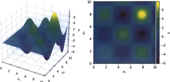
We use a handful of common "test" functions which are low-dimensional and where we

actually know the analytic form. This makes it easier, especially for the functions that

we can visualize directly, to understand what each acquisition function is doing and see

where they fail. These are the Alpine2, Bohachevsky, Branin, Gramacy, Goldstein, Hartmann3, and Hartmann6 functions. Those which are 1- or 2-dimensional are

plotted in Appendix A.

4.1.2

Dataset Maximization Tasks

Because of the expensive nature of applications where Bayesian optimization is used, it is not always possible to evaluate an objective function multiple times to compare

Name Description Dimension

Gramacy

f(x)

= - " +07

+

(x - 1)4 1

Alpine2 f (x)

=

v/

»-isin(xi)

2

Bohachevsky

f(x)

= - (0.7 + X2 +

2x2

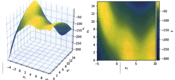
- 0.3 cos(37rxo) - 0.4 cos(47rx1)) 2 Branin f(x) = - ((x1 - X2 +

$xo

- 6)2 + 10(1 -

)

cos(Xo) + 10) 2

Goldstein Appendix A 2

Hartmann3 Appendix A 3

Hartmann6 Appendix A 6

Abalone Predict age of abalone from features. 8

DNA Binding Identify strongly-binding DNA sequences. 32

Robot Push Identify parameters for 2 robot hands pushing 2 objects. 14 Trajectory Identify trajectory points for minimal-cost path. 60 Table 4.1: Overview of the objective functions. xi denotes the i-th dimension of the input point x. Some of these functions have been negated so that they are maximization problems when traditionally they would be minimizations. Alpine2 is defined for any number of dimensions, but we use it in 2 dimensions. Formulas that are excessively long are deferred to the appendix.

different methods. Given an existing set of inputs and outputs from a function, we can simulate optimizing the function by attempting to find the input among this set with the largest corresponding output. As usual, a random subset of these points are sampled to begin Bayesian optimization. At each subsequent step, only the points in the dataset are considered for acquisitions. This lets us evaluate many methods on the same task without the expense of running many physical experiments.

We consider a couple of different dataset maximization tasks in this work.

Abalone The Abalone dataset consists of 8 features (such as diameter, height, and weight) of a few thousand abalone (sea snail) organisms as well as the age of each [381. This dataset has been used previously in Bayesian ptimization either as a prediction task [28], where the hyperparameters of a model t~lat predicts age from the features are tuned using Bayesian optimization, or directly as a dataset maximization task [8]. We adopt the latter setting. Maximizing the function consists of identifying those features of an abalone which lead (in the given dataset) to an organism with the greatest age.

DNA-binding Proteins We use the DNA-binding experiments from [1] as a set of objective functions. These experiments measure how strongly different proteins (tran-scription factors) bind to given 8-basepair DNA segments. There are 38 tran(tran-scription factors in this dataset; we sample five of them to use here (each can be considered a separate objective function). These experiments have evaluated all approximately 32,000 possible inputs, so our methods are able to acquire any possible point in this space. We represent each basepair as a vector of length four with has zeroes at all positions except a one at the index corresponding to the basepair. DNA sequences are represented as a 32-dimensional vector which is the concatenation of the 8 one-hot vectors for each basepair.

4.1.3

Simulations

Robot Pushing This is a task defined on a simulated robot introduced by [55]. The robot is composed of two hands and the goal is to push two objects into a specific location. The input parameters specify things such as the location, rotation, and velocity of the robot hands.

Rover Trajectory This task was introduced in [53] and emulates a 2D rover navi-gation task. The goal is to define a trajectory from a start location to a target location by giving the coordinates of 60 points along that trajectory (to which a BSpline is fit to determine the intermediate locations). A predetermined cost function is integrated across the trajectory to determine the reward.

4.2

Baselines

For comparison, we use two random acquisition functions as baselines. The first selects points uniformly at random from the input space (in the case of a finite input space, this is uniform among the points not yet acquired). The second selects all points at once using Latin hypercube sampling with multi-dimensional uniformity (LHS-MDU) and then returns the next b points each time a batch is to be acquired (selecting