on the Taguchi Method
by
Shih-Hung Li
S.B., Mechanical Engineering (1990) University of Texas at Austin
Submitted to the Department of Mechanical Engineering in Partial Fulfillment of the Requirements for the degree of
Master of Science in Mechanical Engineering
at the
Massachusetts Institute of Technology
January, 1992
QMassachusetts Institute of Technology 1992 All rights reserved
A
Signature of Author
Department of Qechanical Engineering January 17, 1992 Certified by - W -Dr. Haruhiko Asada, Professor Thesis Supervisor Accepted by
Chairman, Department Committee
AF , -,, E.f1iU', EIS ISTITUTE O)F T''r 're.,1 <!qv1 F~L- D 3: 0 1992
Er
Dr. Ain A. Sonin on Graduate Students MIT LIBRARIES AUG 0 3 1992 BARKER ---.-__-Or - --Automated Robotic Assembly Using a Vibratory Work
Table:
Optimal Tuning of Vibrators Based on the Taguchi Method
by
Shih-Hung Li
S.B., University of Texas at Austin (1990)
Submitted to the Departmelnt of /Mechanical Enginceri'ng o .January 7th, 1992 in partial fulfillment of the requirements for the Degree of Master of Science in Mechanical Engineering
Abstract
The goal of this paper is to perform complex assembly tasks, using a robot assisted by a multi-axis vibrator that reduces friction and avoids jamming. An experiment-based approach using the Taguchi Method is applied to the tuning of the vibrator. The vibrators are tuned so that effects of friction and stick-slip can be minimized. Using actual assembly data and an experimental analysis method, called Taguchi analysis, we obtain optimal settings for the vibrator through an iterative procedlure. The use of Taguchi Method is a new learning technique. The Taguchi Method has brought the true meaning of automation to reality by eliminating human intervention in operating the control console. A minimum number of tests or experiments are designed and conducted at each iteration, and the process is repeated until final results reach a satisfactory level. To evaluate performance, we use the root mean square of reaction force and moment during assembly, which indicates the magnitude of stick-slip and the effect of friction. The basic technique, a prototype system, and experimental results are presented in this paper. After we have proven the concept of using Taguchi Method as a new learning method, we then apply it, to two dimensional cable connector assembly. The experimental setup and results are also presented.
Haruhiko Asada
Thesis Supervisor: Haruhiko Asada
Professor Mechanical Engineering, MIT
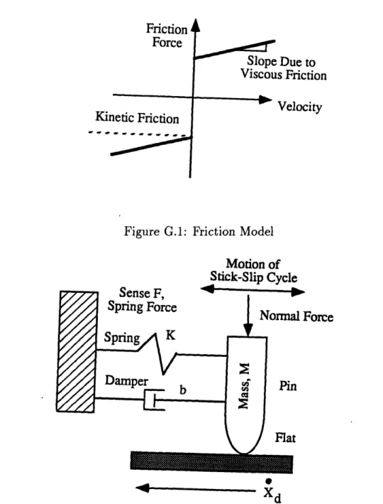
G.1 Friction Model
G.2 Schematic of R.abinowicz Friction Model ...
G.3 Typical example of stick-slip force plot ...
G.4 The simplified schematic of the total working systelll . . . G.5 Block diagram of a product/process ...
G.6 Flowchart for the data acquisition ... G.7 L32 orthogonal array ...
G.8 Input setting for the 1,32 ... G.9 Orthogonal array used for the experiment .
G.10 Flowchart to automating the Taguchi Method ... G.11 Cable connector experiment set-up ...
G.12 Robot used for the experiments ... G.13 Connectors used in the experiments ... G.14 Data, acquisition diagram ...
G.15 The robot assembly trajectol ry ...
G.16 A plot of a typical force trajectory together with its original G.17 Force and position plots for non-contact robot motion . . G.18 Force and position plots for non-vibratory robot motion . G.19 Force and position plots for robot motion in optimal settings
... . .49
.. .... .50
51 . . . 5 1... . .52
... . .53
.54...
...
55
.56... . .57
... . .58
.59... . .60
... . 61
data . . 62... . .63
64 65 49 iAutomated Robotic Assembly Using a Vibratory Work
Table:
Optimal Tuning of Vibrators Based on the Taguchi Method
by
Shih-Hung Li
S.B., University of Texas at Austin (1990)
Submitted to the Departmc'nt of lMechanical Enginecrilng o Jantuary 17th, 1992 in partial fulfillmzent of the requi'rlcm ie nt.s for the De:/l ol M.lstc of Science in MIechanical Engileeri'ng
Abstract
The goal of this paper is to perform complex assembly tasks, using a robot assisted by a multi-axis vibrator that reduces friction and avoids jamming. An experiment-based approach using the Taguchi Method is applied to the tuning of the vibrator. The vibrators are tuned so that effects of friction and stick-slip can be minimized. Using actual assembly data. and an experimental analysis nietliod, calle(l '.I'agtcli analysis, we obtain optimal settings for the vibrator through a it,erative procedult.e. The use of Taguchi Method is a new learning technique. The Taguchi Method has brought the true meaning of automation to reality by eliminating human intervention in operating the control console. A minimum number of tests or experiments are designed and conducted at each iteration, and the process is repeated until final results reach a satisfactory level. To evaluate performance, we use the root mean square of reaction force and moment during assembly, which indicates the magnitude of stick-slip and the effect of friction. The basic technique, a prototype system, and experimental results are presented in this paper. After we have proven the concept of using Taguchi Method as a. new learning method, we then apply it to two dimensional cable connector assembly. The experimental setup and results are also preselltedl.
Thesis Supervisor: Haruhiko Asada
Professor Mechanical Engineering, MIT
i
Some people entertain ideas, others put them to work.
IAcknowledgement
I am most grateful to my parents who made a most crucial decision to send me abroad eight years ago. If not for that decision, I am sure that I would not be what I am now. I would like to thank them and my sister for the many sacrifices they have made for my sake, for giving me emotional and financial support, and most of all, for being there when I needed them.
I would also like to thank my godparents, my "sister", and brothers" who have given me a home and family for the past eight years.
I would like to take this opportunity to thank Matsushita Electric Ltd. for sup-porting this project and to express my sincere gratitude to Mr. Kenji Okamoto for teaching me so much and helping me to understand the hardware in a. such short time. I would also like to thank Mr. Noriaki Yoshida for his assistance.
I would like to express my deepest thanks and respect to Professor Harluhiko Asada., whose painstaking instruction and advice have helped me grow both academ-ically and personally. His unique suggestions and ideas have inspired nme to explore deeper in my studies instead of merely scratching on the surface.
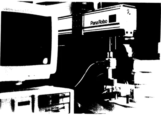
I would also like to thank my colleagues in the Intelligent Machine Laboratory who have given me a great deal of advice and support and have certainly made my stay at the lab a wonderful experience. I would also like to thank the PanasoLic robot who was kind enough to cooperate by functioning normally and the couch in my office which provided a temporary home" for me after late nights at the lab.
I would also like to thank my roommates, (CIhen-an ('heln ad 'ing-Jen Yel for putting up with me for so long. There are so many people I must thank that, it would be impossible to mention you all. I thank all the dear friends I made during my stay at MIT, for giving me the moral support I needed and for helping me in times of need.
1 Introduction
2 The Problem and Approach
2.1 Friction and Stick-Slip in Assembly 2.2 Assembly Using a Vibration Worktable
3 Optimal Tuning using Taguchi Method
3.1 Traditional Learning Methods ... 3.2 Overview of the Taguchi Method . . .
3.3 Self-Tuning Procedure ...
4 Implementation and Experiments
4.1 Data Acquisition ... 4.2 Orthogonal Array ...
4.3 Analysis of the Mean and Variance . . 4.4 Interpretation of the test results .... 4.5 Automation of the Taguchi Method
5 2-D
5.1
5.2
5.3
Cable Connector Insertion
Hardware Setup ... Software Setup ... Experimental Results ...
6 Conclusion and Future Work
viii 1 3 3 5 7 10 12 17 17 17 18 20 21 22 299 23 26 28
...
...
...
...
...
...
...
...
...
...
...
...
...
CONTENTS
A Experimental Results of L32
B Interaction Results for RM1SAI,
C Experimental Result and Analysis of L27
D Taguchi Method [Phadke, 1989]
E The Orthogonal Array Used
E.1 The Standard L9 Orthogonal Array ...
E.2 The Standard L18 Orthogonal Array ...
F Cable Insertion Experimental Data
G Figures ix 31 32 33 35 39 39 40 41 48Introduction
The assembly of printed circuit boards (pc board) has been performed very efficiently by insertion machines. Those assembly machines are operated a.t high speed and low costs, but still have difficulty in dealing with odd-shaped collllolllts such as heat sinks, connectors, and other non-standard parts. Most of those odd-shaped" components are still manually inserted into pc boards, which are a bottleneck of
automation.
Assembly has been addressed by a, number of research groups including [Simunovic, 1979], [Whitney, 1982], [Mason, 1982], [Lozano-Perez et al., 1984], and [Asada, and
Hi-rai, 1990], and [McCarragher and Asada, 1991]. [Whitney, 1982] used
Remote-Center-Compliance (RCC) hand to describe the use of passive compliance as an aid for the
insertion process. [McCarragher and Adada 1991] treated the whole assembly pro-cess as a discrete dynamic propro-cess as compared to the quasi-static propro-cess proposed by [Whitney, 1982]. [Asada and Okamoto] used the neural-network with the back-propagation method to complete the assembly process. [Dulpuis 1992] studied tlhe assembly process by translating human-skills to the machine. T'hese techniques are in general based on compliance and force sensing, which are effective for coping with geometric uncertainty and misalignment. However, difficulties dealing with greater uncertainties arise from to friction. Friction is highly nonlinear, and unpredictable. It disturbs force sensing and smooth operations. The problem becomes harder when we deal with con-plex, odd-shaped parts; they often have burrs ancl unfinished surfaces, which prevent smooth insertion operation a.nd cause jamming.
CHAPTER 1. INTRODUCTION
The goal of this research is to develop a technique for complex robotic assembly using a passive compliance and active vibration worktable. The vil)ratory asselm-bly table assists the robot by generating dither that breaks down equilibrium force conditions between the contact forces and robotic applied forces, thus allowing the workpiece to move smoothly. Our target task is to develop an effective way to tune the vibrator in order to virtually reduce friction and stick-slip. Parameters for con-trolling the vibrator, eg. frequencies, amplitudes, and phases, are optimized by using an experimental robust optimization techniqcue.
In Chapter 2, we will describe the assembly task discussed in this paper. (Chap-ter 3 discusses the reason why the Taguchi Method is implemented and will include a brief overview of the Taguchi Method. A more detailed description of this robust opti-mization technique, also known as the Robust Design, is given in Appendix C[Phadke,
1989]. In Chapter 4, we will explain how we evaluate the assembly operation
quali-tatively and how we actually minimize the performance index. l-D concept prloilng experimental data are also presented in Chapter 4 to support our approach. Chapter 5 presents 2-D cable insertion test results. Finally, Chapter 6 presents the conclusion and future development of this method.
The Problem and Approach
2.1 Friction and Stick-Slip in Assembly
Assembly is the process of mating a geometrically constrained workpiece with its environment. Most of the odd-shaped electronic parts such as heat sinks and connec-tors are made by molding, forming, drawing, or cutting sheet metals and composites. These manufacturing processes result in rough surfaces and edges around the parts. As those parts slide across printed circuit boards during assembly operations, they encounter large frictional forces. These frictional forces often cause unwanted motion such as stick-slip and jamming. In the worst case, the mating workpiece may be permanently damaged or get stuck in the machine. The damaged part halts the as-sembly line, which results in an increase of manufacturing costs. Our main task here is to reduce the chance of stick-slip and jalnming. Therefore, we ineed to ullderst and the physical behavior of frictional contacts and develop a method for quantifying the behavior.
Friction significantly affects performance of almost all the servo-controlled ma-chines. Friction becomes a, dominating factor especially for precise motions at low velocities. Friction determines the range of displacements and velocities at which the mechanismi can operate. The minimum achievable displacement and sustainlable velocity arise from a periodic process of sticking and sliding, a motion called stick-slip. The stick-slip was first studied by [Thomas 1930] using the static plus kinetic friction model shown in Figure G.1. [Bowden and Leben 1939] demonstrated that
CHAPTER 2. THE PROBLEM AND APPROACH
sticking occurs and coined the term stick-slip. However, it has been proven through macroscopic observation that the static plus kinetic friction model is inadequate to explain the observed phenomena. [Sampson et . 1943] [Dokos 1943] [Rabillowicz
19.51] used experiments to indicate that change in friction does not coincide exactly with changes in mechanism state. [Rabinowicz 1951] found that the break-away tran-sition from static to kinetic friction is not instantaneous. He defined the two temporal phenomena involved in stick-slip: rising static friction and frictional lag.
Based on these analysis and experimental results, we consider the one-dimensional model shown in Figure G.2. Velocity, At, represents the relative velocity between the workpiece and the floor, K the stiffness of the robot and the workpiece, and b the damping of the robot. A typical force profile is shown in Figure G.3. This was
ob-tained by sliding a flexible workpiece along a flat surface at a constant speed without vibration. The typical profile of a stick-slip force is shown in the interval from A to C
in the figure. During the stick interval, A-B, the force rises at, a rate proportional to velocity, k Xd, and reaches the static friction at point B. Slipping occurs at interval B-C following the stick region. The exact motion is governed by the mass-spring dynamics as well as friction properties. As the speed increases, the magnitude of the maximum static friction force decreases. This stick-slip condition becomes sig-nificantly noticeable when there is a larger contact force or a higher coefficient of
friction between the two contact surfaces. The ideal "smooth" contact is observed when the stick frequency approaches infinity and the amplitude approaches the nom-inal force. The sticking takes place while the horizontal force is less than the stiction, and slipping occurs when the internal stress force finally exceeds the stiction.
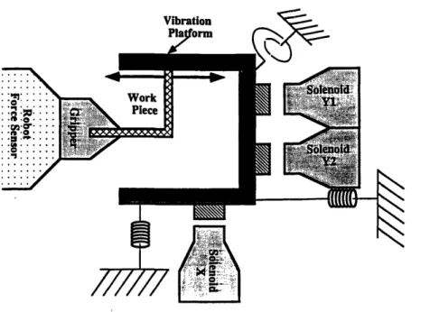
2.2 Assembly Using a Vibration Worktable
Our main goal is to develop an effective method to prevent sticking and jamming and allowing for smooth assembly operations. The technique we use is to generate dither: the one often used in parts feeders and servo controls. Instead of shaking the robot, we shake the worktable that holds a workpiece. We have found that robot actuators are not appropriate for generating dither due to limited durability and power. In contrast, worktables have less constraints and allow us to generate various dithering motions required for assembly tasks.
Figure G.4 shows the schematic design of the worktable considered in this paper. The system consists of an elastically supported platform, three independent solenoids that produce vibrating forces on the platform, and a robot manipulator equipped with a multi-axis force sensor. Each solenoid can generate various patterns of vibra-tion with different frequency, amplitude, and phase. By changing combinavibra-tions of frequencies and amplitudes of the three solenoids, we can create an abitrary vibra-tory motion within a plane. The question is how to find an optimal combination and the optimal vibration modes of these parameters so that the sticking and jammilg problems may be alleviated most effectively. The tuning of the three-axis vibrator comprises of many design parameters and depends upon many factors. Depending on the shape and size of the workpieces as well as their material and surface finish, optimal conditions of the vibrator will be different. Optimal parameters will also be different depending on the trajectory and compliance of the robot. as well as the misalignment between the workpiece held by the robot and the one fixed to the work-talble. These are all relevant factors and conditions, many of which are often unknown or uncertain. It is difficult to obtain a useful analytic model that predicts dynamic behavior of the workpieces and provides optimal conditions for the vibrator. In this
CHAPTER 2. THE PROBLEM AND APPROACH
paper, we will develop an alternative approach to the optimal tuning; an experimen-tal. approach based on the Taguchi Method combined with a recursive optimization technique. First, we take data by having the robot perform a given task under various vibrator conditions. Task performance is evaluated using a performance index. Op-tirnal ranges of parameters are then determined based on the performance index and the data acquired. Within the obtained optimal ranges, experiments are repeated to find better conditions in narrower parameter ranges. This cycle is repeated until the performance index reaches a satisfactory level. To make this operation effective, we need to reduce the number of experiments to be conducted and n-inimize human in-tervention in the optimization and data, acquisition. We employ tlie Taguchi Method and develop an automated tuning system.
Optimal Tuning using Taguchi Method
3.1 Traditional Learning Methods
The traditional learning methods require intensive human intervention in the prelim-inary planning that will enable the controller to "learn" or "acquire" the necessary human knowledge. Two of the most widely used learning algorithms are neural-network and fuzzy logic.
The neural-rnetwork functions in a way similar to how human neurons function. The multi-layer neural-network with backpropagation is an excellent method for learn-ing and predictlearn-ing a nonlinear function as long as a sufficient number of data points are collected from the system and the number of hidden layers and nodes of the net-work is above the minimum required for interpolating the system correctly. Up to now, there is still not a single rule or a guideline we can use to correctly pin down
a minimum yet sufficient neural-network structure for each givell system. Usually, some prior knowledge of the system is required simply to guess the behavior of the system. The network with its too simple structure can not converge and may stay at a local minimum. On the other hand, the network with a more complicated structure can be trained to follow the system smoothly. However, it undermines the noise effect when it is used to predict the outputs and requires a great deal of computation power and time.
The fuzzy logic method is based on the human linguistic rules or guideliiies wl-ich form membership functions. Depending on the inputs of the system, particular rules
CHAPTER 3. OPTIMAL TUNING USING TAG UCHI METHOD
or guidelines are combined to give a single resultant output. It is this fuzziness output which gives merit to this method. Unlike binary logic, fuzzy logic also provides intermediate values between the two extreme values. However, performance of the method depends largely on the number of the linguistic rules and the shape of the membership functions. In order to define these correctly, the user must have an in-depth understanding of the system, usually up to the level of an expert, and needs to go through a time-consuming trial-and-error process to fine-tune the fuzzy controller.
The two methods mentioned above are both non-model-based imet-hods which Ileet the general requirements described in Section 2.2. Both methods require an expert's knowledge in order to sufficiently transfer human skills to the controller. However, not all human "wisdom" is correct as some information may be missing. Therefore, much time is spent working with system identification and parameter estimation, in order to identify the factors that really affect the system or just to get. some insights of the system before we can design the learning algorithm.
System identification deals with the problem of building mathematical models of dynamical systems based on the system data observed. The identification of models from the data, involves decision making on the part of the person in search of models, as well as fairly demanding computations to furnish bases for these decisions. A user typically goes through several iterations in the process of arriving at a. final model, revising earlier decisions at each step.
With a rigorous system identification method and after endless trial-and-error, the parameters involved in the system can be identified. However, the convergence still depends on the consistence of the data signals, and the original parameter structure. The user has to design both the actual planning and the trial-and-error processes. If every thing goes smoothly, the mathematical model will behave like the real system.
However, the set of parameters obtained are considered to be the optimal solution only
to the particular output cost function used. It is not guaranteed that this solution is optimal for a different cost function.
The fine-tuning process of the controller as mentioned earlier requires extensive human intervention. Each data set collected from the system is incidental and subject to the noises that will arise from the system itself and the environment. After fine-tuning the controller to follow a certain data set, we will, most likely, have to redo the fine-tuning when another set of data is considered. Therefore, we may conclude that the controller is not flexible enough to gain on the overall icture. Besides the extensive fine-tuning processes, the preliminary planning of the project also requires human intervention. One practical way of using such a learning method is to combine it with an adaptive controller with a prior model built from the system identification method, as done in work by [Asada, and Liu 1991]. However, the adaptive control is
a, model-based control, thus requiring us to provide an adequate model of the system. Extensive prior knowledge of the system is necessary for preliminary planning of the system.
The traditional intelligent learning methods require human expertise in designing the controller. This involves the design of learning strategies, applying them to ex-perimental data to reduce the system and environment noises, and a. final fine-tuning procedure to adjust the intelligent learning controller. At present, we still refer to systems with intelligent learning controllers as automated systemls. However. if' we consider the overall process as starting with the preliminary planning to the end when the output is obtained, human intervention plays a, very important role in closing the control loop and supervising the controller action. In order to have a, true automation process, we need to search for a. new method to eliminate human involvement within the control loop. The Taguchi method, first. developed by Dr. Genichi Tagauchi in the 1950s and 1960s, can provide the missing link between the Ilunian and the
nma.-CHAPTER 3. OPTIMAL TUNING USING TAGUCHI METHOD
chine controller, thus eliminating the need for human involvement. Our next section will give a brief overview of the Taguchi Method.
3.2
Overview of the Taguchi Method
In Appendix C, we summarize the basic techniques of Taguchi Method, or Robust Design. Here, we will give a brief overview of the Taguchi method and its strengths in designing (experiments. We see the Taguchi Method being applied to the product and process design in the industrial field. The atteml)t here is to apply this special discrete optimization method for the first time to the field of 1illanulfa.ct.urilg cOllt L].
The key idl.ea. the Taguchi method, or Robust Design is to improve the perfornmance of a system, or the quality of a product, by minimizing the effect of the causes of
vari-ation without eliminating the causes. This is achieved by optimizing the product and process designs to make the performance minimally sensitive to the various causes of variation [Phadke, 1989]. The Taguchi Method draws on many ideas from statis-tical experimental design to plan experiments for oltaining dependable information about the variables. Two major tools used in Robust Design are signal-to-noise ratio, which measures quality, and orthogonal arrays, which are used to study many design parameters simultaneously.
With the use of the orthogonal arrays, we can implement a minimum number of experiments in our design. Each different level of the control paranieter appears an identical number of times during the entire experiment set wheii we use orthogoiial arrays, thus enabling us to analyze the data with ease. Unlike the system identification process, there is no longer any human involvement in the experiment design. The preliminary planning process requires knowing only the number of control parameters and noise factors. The noise effects can be taken care of with another noise orthogonal array. I)epending on the time and cost of the experiments, we can either have a
full-blown noise orthogonal array together with a regular control parameter array, which is usually used in simulated experiments; a single combined noise factor or no noise array, which is usually used for design process experiments; or a simplied noise
orthogonal array at actual field noise level, which is used for the process experiments. In this way, the Taguchi Method has automated the preliminary planning process with the use of the orthogonal array. Thus the number of the experiments is guaranteed to be at a minimum and are robust enough to combat the effects of the noise.
With the use of the signal-to-noise ratio and analyses of mean and variance to the desired output, we can easily find the new optimal output setting in conjunction with the use of orthogonal arrays. Because each level of the control parameter appears the same number of times during the entire experiment, these analyses can easily find how each level of the control parameter affects the overall system. Based on the information from the current data, set, the analyses give the optimal settings of control param-eters for the next iteration. The analyses also indicate if any interactions between the control factors exist. Another advantage of the allaly-ses is that the methods also indicate how strongly each factor affects the overall system. T'lius, the analyses can instruct us as to which control parameters are unimportant enough to be eliminated and treated simply as system noise. The system now requires even fewer experiments because the size of the orthogonal array is reduced.
These analyses automatically spell out the desired output and give the direction to the next iteration while the modeled output given by the system identification method has to be interpreted by the user to see if it behaves like the true system output, and requires the search for a new setting, through guesswork and trial-and-error. Like the system identification method, fuzzy logic also requires human ability to analyze and find the new setting. The Taguchi Method, however, guarantees stability and convergence while the neural-network guarantees neither! The most remarkable
CHAPTER 3. OPTIMAL TUNING USING TAG UCHI METHOD
aspect of the Taguchi Method is that it takes the trouble and confusion out of the search for the new setting based on the massive system output.
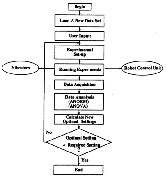
The use of the orthogonal array lets us automate the experimental process through preliminary planning while the analyses offer the optimal control setting. Thus, with the use of the Taguchi Method, we have successfully taken the human factor out of the overall control loop. Because the Taguchi Method is a very systematic method, we can easily implement this method as shown in Figure G.10. In Section 3.3, we will
apply this method to our optimal fine-tuning of the multi-axis vibrator.
3.3
Self-Tuning Procedure
We need to address the following questions found from our optimization method:
* How should we define the performance index that best quantifies the friction and the stick-slip condition?
* How can we apply this method most effectively to mninimize our performance index?
* How should we generalize this procedure to make it autonomous and applicable to other assembly jobs?
We will address each of the questions in this section.
Assembly is the process of mating two workpieces together with geometric con-strains. We define the ideal assembly process as a, process when tile workpiece is
successfully inserted with a minimal number of intermediate steps and a minimal amount of time. Misalignment of the robot or workpiece, variations in parts, and jamrLming or wedging of the workpiece are some important reasons that increase the
number of intermediate steps and the amount of time required in the assembly pro-cess. Sometimes, if the misalignment is too great or the jamming or wedging is too severe, the assembly process will fail completely. The simplest and most cost-effective way of evaluating the assembly process is to keep track of the force information along the assembly process. For a given robot trajectory of an ideal assembly process, we define the ideal force trajectory as the summation of the static forces acting on the workpiece detected by the force sensor a.t each instantaneous time. As we deviate from the ideal case by adding friction, misalignment, variations ill parts, wedging, or jamming to the assembly process, we start, to observe \variations ill thlde force ta-jectory. As we improve the assenbly process, e are i a snse, s llin ilillg lese
variations. Thus we define our performance index as the summation of the root mean square force along the force trajectory. Eq. 3.1-Eq. 3.3 describe how we define them
mathematically.
R(t):q
(ft)-
(t))2(3.1)
(
t=tf T,=
R(t) (3.2) t=O 1 tl.,.(t) =
:f
(t)
(3.3)where R(t) is the root mean square force at an instant tinle, '(1) is the force sensed at the force sensor, m(t) is the average (Idynamic force at all instant time, n is the size
of the moving monitor window for evaluating Eq. 3.3, and the T, is the summation of the root mean square force for the complete insertion process. We minimize this
CHAPTER 3. OPTIMAL TUNING USING TAGUCHI METHOD
In D. E. Whitney's paper, [Whitney, 1982], he uses the peak force value in the direction of insertion as his performance index. His main task is to perform one dimensional insertion of a cylindrical rod. The ideal force trajectory is a constant line along the direction of insertion. Thus we can treat the peak force at each instant time as a special case of the root-mean-square force. As described in [McCarragher
and Asada, 1991], the assembly process is a discrete and dynamic process. Both the magnitude and the direction of the force vector vary quite significantly during the entire assembly process. The force trajectory does not stay constant as the complexity of the assembly process increases, but varies along the trajectory. Thus, looking only a.t the peak f:rce value is not enough to describe a complicated assembly process. It is the variance from the dynamic mean of the force vector that best quantifies the friction and the stick-slip condition. Thus we define our performance index as the summation of the root-mean-square (RMS) force relative to its dynamic mean force, which is also known as the force trajectory. Our optimal solution, or the "smooth trajectory", should minimize this force variation.
Our main objective besides minimizing the friction and the stick-slip condition is to minimize the time and work necessary for the assembly system to arrive at an optimal value. In order to achieve these objectives, we used the experiment-based approach, Taguchi Method, as described earlier in Section 2.2 to obtain this optimal value. The Taguchi Method as based on [Phadke 1989] is described in detail in Appendix C.
(1) Minimizing Time and Work Required
Due to the use of orthogonal array in the Taguchi Method, the minimum number of the experiments we need to perform is (m - 1) x N where N is the number of control factors and m is the number of levels we wish to vary for each control factor.
However, if we use the conventional method, the minimum number of experiments we need to perform is mN in order to have every single combinations possible. For example, if we have three levels for each of the six control factors, we need to run only 12 experiments if we use the Taguchi method instead of the 729 experiments required by conventional methods. Thus, the Taguchi Method saves both time and work in obtaining the optimal values, thus opening up the possibility of running these tests in real time.
(2) Minimizing the Cost Function, SN Ratio
The Taguchi Method uses the Signal to Noise ratio (,S/N ratio) as the main perfor-mance index to arrive at its optimal value. The S/N ratio is the ratio of the mean to the variance in decibel scale, which matches our definition of the performance index. Thus, by usirng the Taguchi method, we can minimize the friction and the stick-slip condition for assembly with a minimal number of tests.
From Appendix C, we see that the Taguchi Method is a very systematic and sequential method. In order to perform each iteration of the Taguchi Method, we need only to supply the following informatioln:
1. Number of control factors (N)
2. Number of variant levels for each control factor (m)
:3. Method selected to optimize the performance index:
* SIB Small value is the best * LIB Large value is the best. * NIB Nominal value is the best
CHAPTER 3. OPTIMAL TUNING USING TAG UCHI METHOD
The method performs the analyses of the variance, mean, and interaction. The method determines the optimal settings based on the current experimental results. From ANORM, the method determines the relative setting of each factor by choosing the highest S/N point for each factor. By using the proportionality of each factor to the overall system in ANOVA, the method can reduce the number of the control factors, thus -further reducing the number of the tests that need to be run for the next iteration and simplifying the control algorithm. The system runs a. confirmation test based on the optimal setting to confirm the results.
(3) Automating the Taguchi Method
After completing the confirmation test, the method can be repeated for the whole pro-cess with a tighter bound around its newly arrived optimal settings than the previous iteration. However, only the ANOVA and ANORM tests need to be repeated since the interaction relationships remain unchanged. This iteration process is repeated until a satisfactory result within the specified tolerance is obtained.
This calibration procedure for the tuning of the multi-axis vibrator is autonomous throughout the entire process. The final optimal settings may be case sensitive for different kinds of assembly jobs. However, the calibration 1)rocedlre is certailly universal for all assembly jobs. This self-calibration process can be 'taught" to fine-tune the settings and adapt to a new assembly job by repeating this method.
Implementation and Experiments
The experimental setup is described in Section 2.2. The vibrations are provided through three function generators to provide a precise vibration amplitude and fre-quency. Our first step is to denlonstrate that vibration in general can reduce the possibility of stick-slip occurrence. The results show that we can effectively reduce RMSM from 50 lb-in (0.576 Nm) for no vibration to 25 lb-in (0.288 Nm). Our next step is to fine tune the vibration system using the Taguchi Method to find the optimal setting for minimizing RMSAlz.
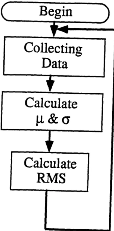
4.1 Data Acquisition
The main purpose of this part is to detect the various slippage occurrences during the sliding motion. The construction of the pattern recognition is based on the flowchart shown in Figure G.6. The data is first acquired through actual experimental data. The pattern recognition is then done off-line. The pattern recognition program (PRP) will calculate the RMS F,, F, and Mll6, and results are then fed into ANORM and
ANOVA.
4.2 Orthogonal Array
The size of the orthogonal array is determined by the number of the control factors. In our case, we have a total of six control parameters: one input vibrating amplitude and frequency from each vibrator.
CHAPTER 4. IMPLEMENTATION AND EXPERIMENTS
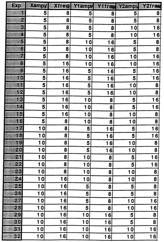
As described earlier, we performed an interaction test to check the correlation between the six factors. In order to study all six interactions, we chose a L32 2-level
orthogonal array for the interaction test presented in Figure G.7. Appendix A shows the results of our experiments. Appendix B shows the interaction plots for ,V'A.l for all six control factors. From the data, we see a strong correlation between Fy1
and Fy2 in the Y direction. This is in fact predictable since they both apply forces in
the y-direction. The only difference between the two is in the direction of the applied moment.
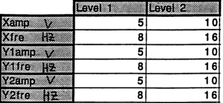
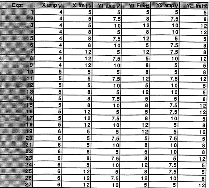
Next, we assigned three levels to each control factor, one on the low, one in the
middle and the last one on the high side from the norm. Based on the information given, we will choose L27 with 7 columns set as dummy columns since L27 was
origi-nally designed to accommodate 13 three-level control factors. The orthogonal array is shown in Figure G.9.
The output of the experiment is obtained from the previouls 1patterli recogllition
program. Once we have all the informlation, we can start analyzi ng the data using
analysis of variance (ANOVA) and aalysis of means (ANOM).
4.3
Analysis of the Mean and Variance
Tl-e main purpose of this analysis is to estimate the effects that each factor has on the final results. First we must calculate the S/N ratio, ?i. Because the main purpose is to minimize the mean and the variance of the rms force and moments, we elect to compute the i? based on the following equation which in turn is based on SIB, small is the best, principle.
= - 10log1 0 ( I (4.1)
N z.=l]
where N is the total number of experiments done for the particle set-up.
After we have computed the S/N value, we need to find the contribution of each level of a particular factor to the overall system. This is easily done lby usinig the orthogonality of the orthogonal array and averaging the S/N values for the set-up for the same level of a particular control factor. Since we have 9 experiments per factor level, the S/N mean for a level A1 is calculated as follows:
( m)
(4.2)Results of' the factor level contribution are given in Appendix C. The one with the highest S/N value of each factor is the one that is least sensitive to noise. The
combination
of Xampl - Xfre
2-Ylampl - Ylfre
3- Y2amp
2- Y2fre
2gives the
highest S/N value.
The next step is to find out how each factor affects the overall system. To do so,
we simply sum the variance of factor level mean to the overall nlean for each factor. For example, the contribution of Xamp is
Vlarx,ap = 9
*
(Xampl-mean)
2+9*(Xamp
2-mean)2
+9* (Xamp
3-mean) 2 (4.3)9 represents the nine experiments done for each factor level. The ratio of each factor
variance to the total variance is the contribution or effect of a particular control factor on the total system. In our case, Y1 amp can take on the highest variation with 81% followed by Xarnp with 8.54%. We can then estimate the optimal S/N value, ?'/opt.
ropt is calculated based on the total mean and the difference in contributions from the upper half of the control factors to the mean. This value of 11,pt is then used to
do linear interpolation to find the optimal setting for each of the control factors. The
7
CHAPTER 4. IMPLEMENTATION AND EXPERIMENTS
7opt = tl7.ean + (amp - l7mealz) + (Ylamp - mzean ) + (12fre - 1/mean ) (4.4)
We can then convert this l/opt back to the estimated RMSMz value as follows
RMSAI =10 (4.5)
Our 7]opt value is -21.05 dB, which gives the RMS1 ,z value of 0.0886 lb-in (0.00102
Nm). Our next step is to run a confirmation test to confirm the test results. Our confirmation test shows a final RMSMZ value of 1.5 lb-in (0.0173 Nm). If we want to further reduce this value, we can repeat the overall process with a band around the optimal setting that is tighter than what we selected from our previous test results.
4.4 Interpretation of the test results
The test results show a 50% reduction in RM,SA', from 50 lb-in (0.576 Nm) where no vibration is applied, to an average of 25 lb-in (0.2880 Nm). After the first iteration by the Taguchi Method, the value was further reduced to 10 lb-in (0.115 Nm). The confirmation test based on the optimal setting from the first iteration has reduced the RiMSz value to 1.5 lb-in (0.0173 Nm). The RASMz value is the criteria we use to evaluate stick-slip, and therefore, by lowering R1lS.,,, we can have a much smoother assembling process which means a lesser chance of stick-slip.
In order to smooth out the motion in the Y direction, we need vibration forces in the X and Y directions together with a moment in the Z direction. The applied moment in each instance opens the gap between the two contacting surfaces thus allowing less chance for the workpiece to stick. An interesting fact is that we need the moment and its frequency but, not its magnitude to reduce the sticking or to keep it from occurring altogether.
4.5
Automation of the Taguchi Method
The Taguchi Method is a very systematic sequential method. It can be nlodified quickly into a learning scheme by using the flowchart shown in Figure G.10. In fact, this is how we obtained our optimal input settings except we have human intervention instead of total automation. By having the user enter the number of control variables and guess the initial optimal settings, the computer then searches for the right orthog-onal array to use. The range of the initial settings is based on the initial intuition of the user. Then the computer performs the experiments. The force data are obtained directly through the robot force sensor. The two analyses are performed. After each iteration, the computer runs a verification test to validate the newly arrived optimal settings. Before the optimal settings are set to start another iteration, the computer checks the relative contributions from each factor to see if reduction on the number of the control factors is possible. The process is repeated until the final op)timal result falls within the tolerance.
Chapter 5
2-D Cable Connector Insertion
After seeing how the Taguchi Method has successfully reduced the stick-and-slip condition in one-dimensional sliding, we apply a completely automated method to do a more realistic and complicated 2-D insertion of a cable mate connector to its female counterpart as shown in Figure G.13. The hardware and software issues will be introduced later in this chapter. The experimental results will be presented as well.
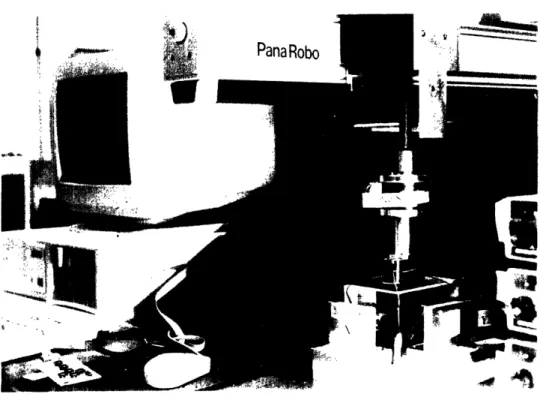
5.1 Hardware Setup
The robot used in the experiment is the PanaRobo AS manufactured by Palasonic Inc. as shown in Figure G.12. It has four degrees of freedom: X. Y. Z. and 0. In this implementation, experiment, we deal only with planar insertion. The robot moves in the X, Y, and 0 directions to complete the insertion.
The complete experimental setup is shown in Figure G.11. The workpiece used ill these experiments is a 25-pin male cable connector, the RS232 Mini-Tester. Our goal is to insert this 25-pin male cable connector into its female counterpart, both of which are shown in Figure G. 13. The multi-axis vibration table sown ill the previous chapter is also used for this experiment.
The .J3force sensor is mounted on the wrist of the robot. This sensor can measure
forces and moments in all directions. In this case, we shall use only the F,. Fy and My
variables so as to adapt to the setup. The control console is controlled by an
compatible Dell computer which runs at 25 Mhz. The control commands are sent directly through the control board of the robot which has its owin built-in position control algorithm. This may create a jiggling motion in the robot and has a dominant effect on the force sensing data and the smoothness of the robot motion.
5.2 Software Setup
The source code of this software program is written in AMicrosoft C and is based on the flowchart shown in Figure G.10. The main program must perform the following tasks:
* Design an appropriate orthogonal array for the experiments
* Run the experiments according to the assigned orthogonal array
* Calculate the root mean square force values with respect to the dynamic mean
* Perform ANOVA and ANORM analyses to find the new optimal values and settings
* Repeat the process using newly assigned settings until performance is at an acceptable level.
More detailed descriptions and the issues involved are presented below.
(1) Preliminary Planning
The preliminary planning segment of the program asks the user for the number of the inputs and the control parameters. Then it assigns an appropriate orthogonal array based on the number of input control parameters. The main purpose of this segment of the program is to design and plan a strategy for the experimental set-up so that the
CHAPTER 5. 2-D CABLE CONNECTOR INSERTION
controller can understand the system after running a minimum number of experiment sets. The sets of orthogonal arrays used here are all standard ones. Appendix E shows two of the orthogonal arrays used for the experiments. This program has been written to accept three to six three-level control parameters. The program assigns a L9 orthogonal array to a system with three or four control parameters and a L18
orthogonal array to a system with five or six control parameters. The user also enters a maximum allowable performance index tolerance so that the program will terminate after it arrives within the specified window. The user is also required to enter the maximum number of iterations just in case the program does not reach the specified tolerance within a reasonable time interval.
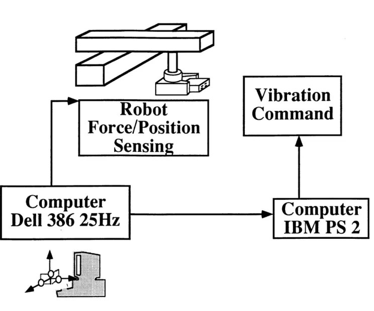
(2) Data Acquisition
The main tasks of the data acquisition segment of the program are to send amplitude and frequency values to the vibrators and to move and control the robot while it takes force and position data. These tasks can be found in Figure G.14. Due to the present limitations of hardware in the computer architecture, the vibration comlmands can not be sent directly to the vibrators; instead, they are p1reselte(l ol the sc(reel and require human aid to set them up. Even though the controller requires human intervention, it does not require a decision on the part of the human. The robot motion is predetermined and the controller performs a. very simple trajectory control in conjunction with the logical branching [Li, 1991]. The robot motion follows a trajectory as shown in Figure G.15. A simple logical branching algorithm is added
to the control loop monitoring robot motion. The purpose of the logical branlllillg algorithm is to ensure that the robot reaches a specified contact state or remains at that state, but does not arrive at a danger contact state. Our main purpose is to use the robot to acquire data. Therefore, the robot trajectory control algorithm is kept 24
at minimal complexity. All the force and position data of each experiment are stored in different files. Approximately 600 to 700 sets of data are collected during each trial and the sampling time is approximately 2ms.
(3) Evaluating the Performance Index
The performance index as defined earlier is the minimum root mean square forces. Our first step is to define how we actually obtain the values of the root mean square force in this case. In order to ensure that the root mean square values we obtain are valid, we must look into the force trajectory. A simplified definition of the force trajectory is found by taking the instantaneous values of the dlynaml-ic mean or average force value within a moving monitor window. The square variation from the mean is our definition of the root mean square. An important issue here is how to determine the size of the dynamic monitor window. An appropriate window size captures the true force variation without concerns about whether it is too sensitive or too static to the changes in force data. A typical force data plot and its force trajectory is plotted in Figure G.16. We find that the ideal size of a dynamic monitor window that will give the most, accurate values of the root mean square is 100. After the robot switches contact states, the dynamic mean values are recalculated based only on the force data obtained at the new contact states to ensure their validity.
(4) Minimizing the Performance Index
The analyses of the mean and variance segment of the programn are exactly the same as those presented in Section 4.3. The final optimization segmlent of the program is also similar to the material presented in Section 4.3. The program assigns different new settings for each level. This is done to ensure that the final optimal value is an absolute and not a local minimum. If the signal-to-noise ratio is highest for either
CHAPTER 5. 2-D CABLE CONNECTOR INSERTION
the lowest or highest level of a particular control parameter, the three new settings are shifted by a distance from that level to the original mean, with no change in the variance. On the other hand, if the central setting gives the highest signal-to-noise ratio, it remains at its previous position and the variance is cut down to half of its original magnitude. This whole process is repeated until the root mean square forces reach an acceptable level.
5.3 Experimental Results
Before we run the entire program, we first obtain two data, sets. The first data set is found by running the robot through the trajectory without making any contact as shown in Figure G.17. The second data set is obtained by running the robot through the trajectory without vibration as shown in Figure G.18. Figure G.19 shows the force and position plot obtained by using the optimal settings obtained after the first iteration of the Taguchi experiment set. The first. complete experimental analysis is presented in Appendix F. After completing the first iteration, we have effectively reduced the magnitude of the peak force by half by switching from random vibration to tuned vibration. We have also reduced the peak root mean square force and moment from 10.545 lb for no vibration to 2.5 lb) for untuned vibration, and 1.5 lb for tuned vibration after the first iteration.
WVe have shown here that the Taguchi Method works or two dlinensiollal cable insertion. However, instead of a single force performance index as for the case of
one dimensional insertion, we now have three performance indices (root mean square force in the X and Y directions and Moment in the Y direction). At present, we treat them as three separate performance indices in our analyses. Fortunately, they predict the same settings for all output parameters except one in spite of different output signal-to-noise ratios. We need to direct our work toward background research and
finding a Taguchi optimization for multiple performance indices.
In the previous chapter, we describe the basic methodology and how it call be applied through a very simple and primary case study of -D sliding. In order to apply the same Taguchi Method to the 2-D cable connector assembly process, we must clarify the definitions and assumptions used.
The experiments are run under several assumptions, which are fixed robot trajec-tory, fixed contact states, and no variations in parts. However, small variations in trajectory are unavoidable when the experiments actually take place. At present, we treat any unavoidable or uncontrollable variations as built-in noises. If time is allowed, a more robust orthogonal array should be iplemented. Besides using an orthogo-nal array for the control parameters, we should also incorporate a noise orthogoorthogo-nal array to account for any "noise" we encounter in case of misalignment, variation in workpieces, and so on. However, we may sacrifice efficiency by requiring more
exper-iments. The optimalization we arrived at is then optimized glol)ally. At present, the optimization is obtained off-line and can not respond to any spontaneous change or variation. In order to obtain a more robust algorithm, we will implement a hybrid controller which will use the Taguchi Method to obtain off-line optimized settings and the learning algorithm to optimize on-line variations. The Taguchi Method can provide a excellent starting point for on-line learning and training, thus eliminating the need for blind guesses.
Chapter 6
Conclusion and Future Work
In the manufacturing process utilizing robotic precision assembly today, stick-slip condition and jamming have severely limited the rate of robot assembly. Due to the complexity of the assembly task, force control itself is not totally effective in a complex assembling process. The visual systems help but have proven to be too slow and expensive. In order to reduce the chance of jamming and sticking, we tried to use a multi-axis vibrator together with passive compliance built into the worktable. The primary reason for adding both the compliance and vibration to the worktable is so that we will not complicate the original system while effectively reducing both detrimental effects.
The new contribution that we make here is to bringing the true meaning of au-tomation to reality, unlike the past, when the automated system was defined as a system that could perform its duty without human supervision. The advance in ar-tificial intelligence (AI) is what makes this possible. The most frequently used AI techniques are neural-network, fuzzy logic, and the expert system. In order to apply these intelligent control algorithms to the design of a, control system, a great amount of man-power is spent to understand the system, to acquire knowledge from experts, to analyze data, and most importantly, to go through an almost endless trial-and-error process once the controller is built. Sometimes, a hybrid controller is constructed by combining the intelligent controller together with an adaptive controller that uses a system identification technique. If we step up one layer and look at, an overall picture of the automation system by considering all the processes that require human
vention as part of the so-called automation process, we soon realize that the human factor acts either as a black box to close the old definition of an automated controller, or acts as God to supervise or oversee the overall control system. Therefore, the au-tomation process defined earlier can only be considered as a semi-automated process. This new process, the Taguchi Method, replaces the human role in the overall control picture and brings true meaning to the automation process. The use of the orthog-onal array in planning the strategy for understanding the system keeps the amount of time and the number of experiments required at a minimum. With the analyses of the mean and variance, the system obtains settings that give better performance. By repeating this process, the system can obtain optimal settings for its control pa.-rameters. Therefore, there is no human involvement in the decision making process.
We now have a true automation process with machine intelligellce obtaiiied 1)! the machine itself' not by a human.
Instead of' using a model-based approach to control the multi-axis vibrator, we use an experimental approach based on the Taguchi Method. The problem with a model-based design is the complexity of equations where many assumptions have to be taken in order for the model to behave like a real system. However, many of
the disturbances or non-modeled factors may still destroy the reliability of the model when the model meets the challenge of the real system. With the help of the Taguchi Method, we can find an optimal solution with a, very limited number of experiments to reduce stick-slip condition with a strong ability to reject outside noises. In comparison
with other experimental approaches the Taguchi Method guarantees convergence as compared to the neural-network nlethod, involves less gulesswork than fuzzy logic, and does not require as many experiments as Monte-(.arlo's Illetllod.
The use of vibration has effectively reduced 50% of the RAi'Sh value from 50 lb-in (0.576 Nm) to an average of 25 lb-in (0.288 Nm). After the first iteration by the
CAILPTER 6. CONCLUSION AND FUTURE WORK
Taguchi method, it was further reduced to 10 lb-in (0.115 Nm). The confirmation test based on the optimal setting from the first iteration has reduced the RMSA, to 1.5 lb-in (0.0173 Nm). The R lSMz value is the criteria we used to evaluate stick-slip and by lowering RMSMz, we can have a much smoother assembly process which means a lesser chance of stick-slip and jamming.
We also demonstrated automated methodology in the use of a more complicated
system--two dimensional cable connector insertion. The repeatability and reliability of the insertion process have been greatly improved, and our next step is to generalize the methodology to perform optimization of a system with multiple performance indices. In order to build a more robust controller, we need to implement a hybrid controller. However, more research work need to be undertaken in future studies combining the off-line tuning using the Taguchi Method and on-line tuning using learning methods.
Experimental Results
of L
32
Data U. 0. U.j3051ZU 0.401373 42.437 0.533244 0.326157 30.3540: 0.469799 0.399991 24.88367 0.669109 0.495550 33.4168C 0.639030 0.335623 35.9423( 0.487262 0.344898 30.1057( 0.546419 0.309265 · 20.0178: 0.800507 0.286761 40.6030 3.318488 55.184784 40.58451 0.570114 0.170395 29.1203, 0.496368 0.216509 25.1627: 2.729831 49.571873 43.8133! 0.764962 0.379940 51.111 0.538099 0.297763 24.441 0.628073 1.806185 0.376220 1.773521 37.941 87. 0.593186 0.402782 27.428150 0.564587 0.283399 32.497720 0.561635 0.380465 31.14754C 0.633752 0.414638 26.36662( 0.724103 0.478380 24.19701( 0.515954 0.325968 27.45624( 0.593478 0.379757 31.18777( 0.794202 0.426320 35.49881. 1.578377 0.464028 17.04812' 42.593395 218.632629 37.064381 0.698332 0.410019 72.59051( 1.116601 0.834322 103.75142( 1.187962 0.580639 101.41749( 0.962306 0.390042 78.18045( 1.099293 0.306379 62.93879( 1.953383 0. 0.3355641 22.7982101 1.460050 0.387565 16.587378 1.413327 0.303531 15.266325 0.629917 0.539315 34.764690 1.208122 0.962160 88.251120 0.920129 0.574406 6.567560 0.925985 0.431937 60.655120 3.560699 0.602823 48.845657 3.569572 0.618212 54.496500 2.125860 0.317944 29.524176 2.042527 0.379212 31.324150 0.692088 0.378687 51.508930 0.733450 0.386313 43.974640 0.543610 0.259344 32.554280 1.054100 0.298853 89.733850 0.789585 0.356599 57.399760 0.733450 0.386313 43.974640 0.543610 0.259344 32.554280 1.054100 0.298853 89.733850 2.784378 0565457 30.829151 1.575221 3.331307 22.195351 1.892658 0.533320 23.06059' 12.362161 66.581535 11.17339' 3.200601 0.498824 45.24812' 3.357237 0.472298 45.22305: 2.663130 0.305415 34.91416' 2.256656 0.268436 32.92143 0.991634 0.286065 47.29563( 1.031742 0.206514 68.13152( 1.071779 0.694098 45.03786( 0.691289 0.311682 45.40636( 31 DataAppendix B
Interaction Results for RMSMz
-12 -14 " -18 m -20 -22 -24 -26 -28 In 15 10 5 0 -5 -10 -15 -20 -25 Ir
Interaction Plot between Xamp vs Y2amp
.. : .. . .. . . . .. . . .. .. . ..'- . ....-i i i 6 -,.oXampl I- !I - -Xamp2 - if
t t '!
i i IIE~l---
-
i '_ ! !:
x
·
6 = 8 :E_~ .,"L~~~~~~~~~I
7 4 5 6 7 2mp8 9 10 11teraction Plot between Xlamp vs Ylamp
i =
4 5 6 ,i am8 9 10 11
interaction Plot between Ylamp vs Y2 amp
i --- i- e -Y1amp2 ---'-'-'i :amp2 4 5 6 lam? 9 10 1 10 11 32 -14 -16 '-18