Modelling European winter wind storm losses in current and future climate

DOI 10.1007/s10584-009-9712-1

Modelling European winter wind storm losses

in current and future climate

Cornelia Schwierz· Pamela Köllner-Heck · Evelyn Zenklusen Mutter· David N. Bresch · Pier-Luigi Vidale· Martin Wild · Christoph Schär

Received: 12 September 2007 / Accepted: 27 August 2009 / Published online: 25 November 2009 © Springer Science + Business Media B.V. 2009

Abstract Severe wind storms are one of the major natural hazards in the

extra-tropics and inflict substantial economic damages and even casualties. Insured storm-related losses depend on (i) the frequency, nature and dynamics of storms, (ii) the vulnerability of the values at risk, (iii) the geographical distribution of these values, and (iv) the particular conditions of the risk transfer. It is thus of great importance to assess the impact of climate change on future storm losses. To this end, the current study employs—to our knowledge for the first time—a coupled approach, using output from high-resolution regional climate model scenarios for the European sector to drive an operational insurance loss model. An ensemble of coupled climate-damage scenarios is used to provide an estimate of the inherent uncertainties. Output of two state-of-the-art global climate models (HadAM3, ECHAM5) is used for

C. Schwierz (

_B

P. Köllner-Heck· D. N. Bresch

Swiss Reinsurance Company, Zürich, Switzerland Present Address:

P. Köllner-Heck

Federal Office for the Environment, Berne, Switzerland Present Address:

C. Schwierz

Seminar for Statistics, ETH Zürich, Zürich, Switzerland Present Address:

E. Zenklusen Mutter

WSL Institute for Snow and Avalanche Research SLF, Davos Dorf, Switzerland Present Address:

P.-L. Vidale

present (1961–1990) and future climates (2071–2100, SRES A2 scenario). These serve as boundary data for two nested regional climate models with a sophisticated gust parametrization (CLM, CHRM). For validation and calibration purposes, an additional simulation is undertaken with the CHRM driven by the ERA40 reanaly-sis. The operational insurance model (Swiss Re) uses a European-wide damage function, an average vulnerability curve for all risk types, and contains the actual value distribution of a complete European market portfolio. The coupling between climate and damage models is based on daily maxima of 10 m gust winds, and the strategy adopted consists of three main steps: (i) development and application of a pragmatic selection criterion to retrieve significant storm events, (ii) generation of a probabilistic event set using a Monte-Carlo approach in the hazard module of the insurance model, and (iii) calibration of the simulated annual expected losses with a historic loss data base. The climate models considered agree regarding an increase in the intensity of extreme storms in a band across central Europe (stretching from southern UK and northern France to Denmark, northern Germany into eastern Europe). This effect increases with event strength, and rare storms show the largest climate change sensitivity, but are also beset with the largest uncertainties. Wind gusts decrease over northern Scandinavia and Southern Europe. Highest intra-ensemble variability is simulated for Ireland, the UK, the Mediterranean, and parts of Eastern Europe. The resulting changes on European-wide losses over the 110-year period are positive for all layers and all model runs considered and amount to 44% (annual expected loss), 23% (10 years loss), 50% (30 years loss), and 104% (100 years loss). There is a disproportionate increase in losses for rare high-impact events. The changes result from increases in both severity and frequency of wind gusts. Considerable geographical variability of the expected losses exists, with Denmark and Germany experiencing the largest loss increases (116% and 114%, respectively). All countries considered except for Ireland (−23%) experience some loss increases. Some ramifications of these results for the socio-economic sector are discussed, and future avenues for research are highlighted. The technique introduced in this study and its application to realistic market portfolios offer exciting prospects for future research on the impact of climate change that is relevant for policy makers, scientists and economists.

1 Introduction

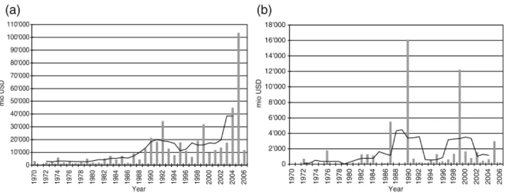
The insured natural catastrophe losses due to atmospheric hazards have increased steadily over the last 30 years. An account of the evolution of annual worldwide weather-related insured natural catastrophe losses is given in Fig.1a. In the 1970s the mean yearly insured losses amounted to approximately 2–3 billion (bn) USD while in the last couple of years (2001–2006) the average value increased to more than 30 bn USD (all figures in 2006 prices). Potential factors contributing to this rise are found in economic, geographic and demographic sectors and comprise: -increasing assets at risk due to rising population and insurance density, -larger concentrations of values in exposed areas and thus higher degrees of vulnerability. It is widely accepted that the world’s climate is changing which results in significant alterations of regional weather and climatic conditions (e.g. IPCC2001,2007), and the potential for a climate-change induced increase of atmospheric hazards has been recognized

(a) (b) 0 10'000 20'000 30'000 40'000 50'000 60'000 70'000 80'000 90'000 100'000 110'000 1970 1972 1974 1976 1978 1980 1982 1984 1986 1988 1990 1992 1994 1996 1998 2000 2002 2004 2006 Year mio USD 0 2'000 4'000 6'000 8'000 10'000 12'000 14'000 16'000 18'000 1970 1972 1974 1976 1978 1980 1982 1984 1986 1988 1990 1992 1994 1996 1998 2000 2002 2004 2006 Year mio USD

Fig. 1 a Annual worldwide weather-related insured natural catastrophe losses (flood, storm,

drought, cold and hail) 1970–2006 (USD mio, prices 2006), b Annual insured windstorm losses for Europe 1970–2006 (USD mio, prices 2006). 5-year-running-averages overlaid (black). Source: Swiss Re sigma Catastrophe database

by the insurance industry for some time, e.g. Berz (1993), Changnon et al. (1997). The degree to which the rise in catastrophe loss can be attributed to climate change has not yet been quantified. Hence, from both a societal and an economic perspective, it is crucial to determine the extent to which changes in a warmer climate could further add to the damage figures.

The focus of this study is on European winter storms. Figure1b is the analogue

of Fig. 1a, but for winter storm losses in Europe. These exhibit a much stronger

variability (volatility). Since 1970 there have been 70 severe wind storm events resulting in total insured losses of approximately 50 bn USD. The thirteen most severe storm events alone account for nearly 80% (or 40 bn USD, in 2006 prices) of total insured winter storm losses in this period. The volatility of losses is exacerbated by the clustering of severe storms, with four in 1990, and three in 1999. In 1990, the total insured loss resulting from four winter storms amounted to 14.6 bn USD, caused by Herta (1.3 bn USD), Vivian (4.9 bn USD), Wiebke (1.2 bn USD) and Daria (7.2 bn USD). In 1999, Anatol (2.3 bn USD), Lothar (7.0 bn USD) and Martin (2.9 bn USD) caused an insured loss of 12.2 bn USD (all in 2006 prices).

According to the Swiss Re loss model, an insured storm loss in the order of some 7 bn USD can currently be expected to occur in Europe about once every ten years while one of 30 bn USD is anticipated once every 100 years (see also

Fig. 2). Other insurance models yield similar damage-frequency relations. History

has shown that winter storms can engender huge losses and insurance models suggest that even higher losses are possible. Most of the operational insurance models are based on historical data. Monte-Carlo-like sampling techniques are then applied to

obtain a comprehensive data base (see Section2.2for the description of the Swiss

Re loss model). For a more realistic risk assessment, especially when taking into account impacts of future climate change, it is highly desirable to link the insurance model with a three-dimensional dynamical climate model. This would allow a more physically-based estimate of current and future annual expected losses and loss potentials to be derived.

The aim of the study is to quantify wind-storm losses on a European-wide property insurance portfolio, under current and future climatic conditions. The study involves

Katrina 2005 45 8 Mireille 1991 8 Daria 1990 Storm Europe 30 Typhoon Japan 15 Hurricane US and Caribbean 120

Nat cat events (indexed to 2006)

Loss potentials from events with a return period of 100 years

Insurance loss potentials in USD billions:

Fig. 2 Insurance loss potentials for weather-related hazards (100 year return period events) and

largest historical insured losses (in USD bn, 2006 prices)

two steps: First, using output from a series of climate models, we analyze changes in surface wind speed and in the frequency of heavy windstorm events. Second, using an insurance loss model, we determine the impact of these changes on insurance losses. It is crucial to study both these factors in combination. Increasing losses are not an inevitable consequence of potentially increasing wind intensity and/or frequency in a warmer climate. The loss amount of a particular storm depends on both its path and its absolute force. It is important to determine (i) whether a storm affects a region with a high concentration of values or passes over sparsely populated territory, and (ii) to what extent and within which intervals the wind intensity changes, as small changes in hazard intensity may trigger substantial changes in damages, due to a nonlinear relationship between atmospheric conditions and inflicted damages.

A number of factors will determine the response of mid-latitude cyclone activity and winter storm frequency to global climate change. Some of the key physical issues are: First, the geographic distributions of near-surface temperature and sea-ice imply pronounced modifications in the low-level temperature contrast (baro-clinicity), which in turn affects the strength and location of the storm tracks (Held

1993). As polar regions tend to warm stronger than the tropics, climate change

diminishes the overall equator-to-pole surface temperature contrast, suggesting an overall decrease in cyclone activity. However, there is a competing effect as the upper-level baroclinicity may strengthen. In this way characteristic atmospheric circulation patterns such as the North Atlantic Oscillation might also be affected

(Ulbrich and Christoph 1999). Second, as the atmosphere warms, it also becomes moister. This moistening effect is expected to approximately follow the Clausius-Clapeyron relationship, thus suggesting a sizeable moistening of about 6% per

degree warming (DelGenio et al. 1991). A moister atmosphere implies that the

equator-to-pole transport of latent heat (water vapor) will increase at the expense

of the sensible heat transport (Boer 1995). Similar to the reduced amplitude of

the equator-to-pole temperature contrast, this factor thus points towards an overall reduction of cyclone activity. Third, it is important to note that a reduction of mean cyclone activity does not necessarily imply a reduction in the frequency of deep cyclones and associated winter storms. In particular, there is ample evidence from the meteorological literature that atmospheric humidity plays a key role in spinning up extratropical cyclones, e.g. Wernli et al. (2002). This spin-up effect is most effective

below the level of maximum condensational heating (Hoskins et al. 1985). The

anticipated moistening of the atmosphere might thus favor a low-level strengthening of extratropical cyclones with potential implications on near-surface wind fields and winter storms.

As the aforementioned factors do work in different directions, comprehensive climate simulations are needed to establish the overall response of the atmospheric circulation. A number of such studies, using climate models of increasing sophistica-tion, have been published in recent years. Overall a fairly coherent picture emerges. On a global scale and for the winter seasons, Geng and Sugi (2003), using a high-resolution GCM, find a poleward shift of the storm track, an overall reduction in the density of cyclones (number of cyclones per area) by almost 10%, and an increase in the number of strong cyclones. The different trends in the counts of weak/moderate versus strong cyclones are confirmed by several other studies (e.g. Carnell and Senior1998; Lambert1995; Knippertz et al.2000; Pinto et al.2007), but not in all of the literature (Beersma et al.1993; Schubert et al.1998). This partly conflicting information will also be assessed in the current study, as we will employ follow-up

versions (HadAM3, ECHAM5) of the models used by Carnell and Senior (1998)

(HadAM2), Beersma et al. (1993) (ECHAM3), Schubert et al. (1998) (ECHAM3)

and Knippertz et al. (2000) (ECHAM4).

It is important to stress that the changes in cyclone activity strongly depend upon the region under consideration. In terms of a regional assessment, a more detailed analysis is needed. Several studies have used high-resolution GCMs and/or limited-area RCMs to focus upon changes in specific limited-areas. Regarding the North Atlantic

/ European sector, Leckebusch and Ulbrich (2004) and Leckebusch et al. (2006)

find an increase in the track density of strong cyclones over western parts of Central Europe. This increase occurs for the IPCC A2 greenhouse gas scenario, but is much less pronounced for the B2 scenario. Consistent with these results, Rockel and Woth

(2007) find an increase of storm peak events by up to 20% over Central Europe

within the next 100 years. As a result, an increase in the frequency of storm surges is expected (Woth et al.2006). The latter increase was simulated using a storm surge model driven by RCMs, and it occurs for most of the North Sea coast with the exception of the East coast of the UK, and for all four RCMs considered.

These extensive results derived in the climate community have yet to find their full application within the modelling approaches of the insurance sector. Watson

and Johnson (2004) provide a comprehensive review on insurance loss models and

wind models in use are parametric models with simple storm parameters, and that the application of climate models had so far not been used operationally due to the computational complexity. However, in a sensitivity study with a representative state-of-the art insurance-type model, they show (for hurricanes) that minor changes in the wind model input parameters (e.g. background surface pressure) can result in significant impacts on the computed loss. They therefore conclude that uncertainties in the wind field propagate dramatically into the damage calculations. A significant improvement can thus be expected with the use of more realistic wind data.

Some studies estimate loss potentials from the available climate model data, e.g. Klawa and Ulbrich (2003), Leckebusch et al. (2007), Pinto et al. (2007). They are based on an approach derived by Klawa and Ulbrich (2003): a loss index is computed based on the excess of wind speed over the upper 2% quantile, and which depends on population numbers in the individual districts within Germany. The calibration is undertaken against publicly available insurance loss data over Germany, which is then applied to other European regions by the later studies. However no operational insurance loss model is utilized in any of these studies.

The present study is one of the first to couple the output from state-of-the-art regional climate models to a slightly modified version of an operational insur-ance loss model. This interdisciplinary approach combines both meteorological and insurance aspects of storms. Consistent with the occurrence of damaging winter storms in Europe, we focus on an extended winter season. In accordance with Swiss Re procedures, this winter season is here defined as October through to March (Oct–Mar).

2 Data and models

2.1 Meteorological data and models

The climate model data utilized in this study has been obtained using one coupled atmosphere-ocean global climate model (GCM), two atmospheric GCMs, and two regional climate models (RCMs) covering all of Europe and a substantial fraction of the North Atlantic. In addition to these climate simulations, we also employ the ERA-40 reanalysis that provides an objective analysis of the observed atmospheric conditions for the time period 1958–2002. The use of different models is meant to provide an assessment of the intermodel spread and thus of the uncertainties of our conclusions. We consider simulations representing current and future greenhouse

gas concentrations, using the IPCC SRES A2 scenario (IPCC 2001). Both periods

comprise 30 years, 1961–90 (CTL) and 2071–2100 (A2) for current and future climatic conditions, respectively.

A considerable fraction of the climate model data employed has been de-rived within the European consortium project “Prediction of Regional scenar-ios and Uncertainties for Defining EuropeaN Climate change risks and Effects”

(PRUDENCE, Christensen et al.2002; Christensen and Christensen2007, see also

http://prudence.dmi.dk/). Therein, systematic ensembles of RCM simulations over the West-Atlantic / European region were conducted at a horizontal resolution of typically 0.5◦× 0.5◦.

The PRUDENCE model chain starts with the Hadley Centre HadCM3, a global coupled atmosphere-ocean model. The HadCM3 simulation is a long low-resolution integration using the observed atmospheric composition for 1859–1990 and scenario

conditions for 1991–2100 (Johns et al. 2003). Mean changes (A2-CTL) in

sea-surface temperature and sea ice from this simulation were used in the subsequent higher-resolution simulations. The next step in the model chain is represented by atmospheric GCMs. We use output of two GCMs, the Hadley Centre HadAM3

(Pope et al.2000) and the Max-Planck-Institute ECHAM5 (Roeckner et al.2003,

2006), both with a resolution of approximately 1◦. These models are run in time-slice mode for the CTL and A2 periods. Prior to the 30 year simulations, 5 years of the simulation have been disregarded to account for potential spin-up effects. The output from the time-slices is used to drive two RCMs, the CHRM and the CLM, at a spatial resolution of 0.5◦and 20 vertical levels.

A total of eight regional climate models (RCMs) are provided by the PRU-DENCE project, but we are using only two of these models. Both the 10 m horizontal wind and 10 m gusts are provided by the PRUDENCE project at daily resolution. The 10 m wind speed represents the daily average length of the wind vector, while the daily maximum length of that wind vector reached during the simulation time interval yields the 10 m gust field. Hence the gust field is much more representative of the maximum speeds reached during a storm event. In a more detailed comparison of the performance of these two input wind fields in our analysis, the gust wind speeds did indeed yield more realistic results. However, it has also been noted that due to the large inter-model differences in the calculation of the maximum 10 m wind, the entire distributions (pdfs) of the gust speeds differ between models by a factor of

10. Rockel and Woth (2007) discuss the problems with the inconsistent 10 m wind

calculations within PRUDENCE. In particular, they analyze and verify the quality of the 10 m gust speeds in great detail. In line with our pdf-analysis they show that only the RCMs that operate a specific gust parameterization (models CLM and CHRM) produced much higher and more realistic gust speeds than the other models. CHRM

and CLM use the same gust parameterization (Schrodin1995) and determine the

maximum wind based on the output of every time step of the simulation. Hence we restricted our analysis to these two models. On a more general note, we add that care is to be exercised in the analysis of gust fields, which typically are not very smooth, and can have large gradients, especially near coast lines, with an increased possibility of grid point wind storms.

The limited-area model CHRM derives from the operational weather forecasting

model HRM of the German and Swiss meteorological services (Majewski 1991),

which has been adapted into a climate version by ETH Zürich (Lüthi et al. 1996;

Vidale et al. 2003). The model is hydrostatic and has a full package of physical

parameterizations, including a mass-flux scheme for moist convection (Tiedtke1989) and Kessler-type micro-physics (Kessler1969; Lin et al.1983). A detailed description of the actual model version and further evaluations are given in Vidale et al. (2003). Here we employ the same model simulations as validated and analyzed in the context

of the PRUDENCE project (e.g. Christensen and Christensen2007) and in recent

scenario and process studies (Schär et al.2004; Vidale et al.2007).

The climate version of the Lokalmodell (CLM) has the same dynamic and physical core as the weather forecast model LM (Lokalmodell) of the German Weather Service (DWD). The CLM is nonhydrostatic and fully elastic. Moist convection is

parameterized by the mass flux convection scheme after Tiedtke (1989) modified by using a CAPE-closure. Prognostic cloud ice parameterization and prognostic TKE scheme are switched on for simulations CTL and A2. For more details refer to Steppeler et al. (2003), andhttp://cosmo-model.cscs.ch/public/model.htm. Again, the CLM simulations used in the current study have previously been analyzed

by Rockel and Woth (2007). Both the CLM and the CHRM are driven at the

lateral boundaries following Davies (1976), using a boundary updating frequency

of 6 h. Sea-surface temperatures are taken from the driving simulation, while soil and snow conditions are interactively established using the models’ land-surface modules.

As an alternative and complementary data source for our analysis, we also per-formed simulations that are not formally part of the PRUDENCE project, but which follow the PRUDENCE strategy in their design: two additional 30-year CHRM simulations (CTL and A2) were nested into the global climate model ECHAM5

(for a description see Roeckner et al. (2006) and companion articles in the same

special issue). The ECHAM5 runs were undertaken at T106L31 using the standard dynamical properties, but PRUDENCE SSTs. For an overview of the realism of the resulting variability patterns cf. for instance Raible et al. (2009). Note that although the SST/sea-ice input for the global atmospheric models is the same, they nevertheless provide additional variability due to different model configurations and formulations. The use of independent global models aids the estimation of the uncertainty inherent in climate model projections (cf. Schwierz et al. (2006)). Thus the analysis presented here is undertaken with the smallest possible multi-model ensemble of three sets of multi-model runs, where the inter-multi-model uncertainties are mimicked to a certain degree by the use of the models CHRM and CLM, while uncertainties due to a variation in the initial and boundary information is partly accounted for by driving the regional models with the two different global atmospheric model outputs.

In an additional simulation the 44-year (1958–2002) re-analysis data set of the European Centre for Medium-Range Weather Forecasts (ECMWF ERA40, Uppala et al.2005) was used as an independent and observationally constrained data source to drive the regional model CHRM, in the same way as for the HadAM3 and ECHAM5 boundary data, but for a longer time period (up to 2001). The dynamical evolution within the CHRM domain closely follows the real development. It can hence be used to develop and test the storm-day selection routine. The resulting criterion is then directly applicable to the climate CTL and A2 simulations, since it is derived with the same model chain rather than from a different (e.g. observational) data source.

In effect, the regional model runs provide a dynamically down-scaled data set that contains much more detail and accuracy than the global models, which is crucial in particular for terrain-dependent parameters such as low-level winds and gusts. Although computationally much more expensive, dynamical downscaling is superior to statistical methods in the sense that the dynamical equations are fully solved and thus the model atmosphere can develop high-resolution features that are dynamically consistent. Also it does not rely on the preparation of an observational predictor data set.

Thus the complete meteorological data set analyzed here comprises gust output from 7 RCM runs, i.e. HC-CHRM, HC-CLM, ECHAM5-CHRM (each with a

CTL and A2), and ERA40-CHRM. Here HC stands for HadCM3/HadAM3 lateral boundary conditions, while ECHAM5 stands for HadCM3/ECHAM5 boundaries. 2.2 Insurance data and models

The proprietary loss model by the Swiss Reinsurance Company is based on four

modules (see Fig. 3): (i) The hazard module is concerned with the location,

fre-quency, intensity and length of the occurred events. The hazard is described with a frequency distribution of different event intensities and duration factors at the model’s geographical resolution. A sample wind gust map (of the maximum intensity in the probabilistic set) is given in Fig.3a. (ii) The vulnerability module accounts for the extent of the damage (mean damage ratio in percent of total sum insured) at a given event intensity. A vulnerability curve is derived from past damage history (cf. Fig.3b) for each risk type (e.g. residential, commercial, industrial and agricultural). (iii) The value distribution describes the amount (total sum insured), location and risk type of the insured values. It is usually available in national administrative districts or sometimes at higher resolution and disaggregated according to population density. (iv) The insurance conditions comprise all the information on the contract conditions that determine the proportion of the loss that is insured. They can for instance encompass deductibles (self-retentions) and damage limits. No such insurance conditions have been applied in the present study for reasons of clarity.

In this study a slightly simplified version of the operational Swiss Re model is employed. It uses an average vulnerability curve for all risk types, and applies only one mean damage ratio value per wind speed, instead of a distribution. The operational model and its slightly simplified version lead to results (climate change

Fig. 3 Swiss Re loss model consisting of 4 modules (see text for details). The sample plots are a

a wind gust distribution of the maximum intensity of the probabilistic set, b a sample vulnerability curve (red line) relating wind gust speed [m/s, ranging between_{∼20–70m/s] to mean damage ratio [%} of total insured value, typically of the order of 0.01%] based on recorded damage history (different symbols and colours are representive of different clients in the residentail sector), c a sample value distribution for several countries in central Europe and the risk types residential (red), commercial (green), industrial (blue) and agricultural (magenta). The resolution varies according to regional administrative borders, and the size of the circle represents the relative value of the asset per regional administrative entity (which varies in size from one entity to the other)

impact) in the same order of magnitude. Details of the operational loss model and the simplifications made for this study are presented next.

In order to simulate a representative and more comprehensive selection of all possible events and to reinforce the statistics of the historical events in the hazard module, probabilistic modeling is used. On the basis of the known historical events and physical parameterizations, thousands of additional hypothetical events are generated by varying the intensity and the track of the storm in a Monte-Carlo-like approach. Whilst these artificially generated events never actually took place historically, there is—from a statistical/scientific point of view—no reason why they should not occur at some point. The hazard module event set typically comprises tens or hundreds of thousands of events, which represent a model time frame of several thousands or several tens of thousands of years. In effect this is the way in which the return periods of particular loss amounts are determined. Such probabilistic sampling models can even take into account the effect of varying climatological conditions such as El Niño or the North Atlantic Oscillation by selecting the corresponding years before applying the Monte-Carlo module.

In this study, the technical details of the hazard module are as follows.

1) The historical event set is the operational one of SwissRe and comprises the

major (143) events (including storms like Anatol, Lothar and Martin) from 1947 to present. These are available as so-called reconstructed “footprints” that are generated using dynamical parameters and relationships, such as the large-scale wind field, the frontal development, the post-frontal low-level jet to adjust for peak gusts, and including observational station data.

2) For the Monte-Carlo method, the historical footprints are spawned, taking the

physical properties into account, through a dual process of (a) rigid motion and rotation and of (b) wind field intensity alteration. To this end the storms have

been intensified/weakened and were shifted in all major directions (+/−50 to

100 km) and rotated (+/−5 degrees) along their axis of movement etc. While

scenarios derived via rigid motion and rotation are considered equally likely, this is not true for those derived via the wind field alteration. In order to have a large enough number of severe storms while not wasting computation time on thousands of almost identical small events, the probability weight of the intensity alteration is different for each historic scenario. In this way, 10 010 events are generated, representing more than 3000 years of data.

3) In order to establish a sound intensity-frequency relationship, a calibration using

the SSI (Storm severity index) according to Lamb and Frydendahl (1991) is

applied. The synthetic storms were assigned probability weights such that the resulting SSI exceedance curve of the probabilistic event set matches the one of the historical event set.

4) To validate the procedure with an independent data set, peak gust return periods from selected meteo stations all across Europe are compared with peak gust return periods resulting from the probabilistic event set.

As a result the probabilistic event set matches well with history and extends it naturally, achieving a very good correspondence of the modeled (probabilistic) compared to observed (meteo stations) gust speeds for a range of return periods.

The vulnerability module (see Fig.3b) takes into account various factors describ-ing the insured risk. As it is not possible to analyze the characteristics of each and

every insured object, classes with common vulnerability curves are defined, which are derived empirically. Figure3b illustrates point data for damage information for a variety of customers with respect to measured wind speed. From this, a mean damage ratio is derived. In order to allow for fluctuations within these categories, a random distribution around the mean damage ratio is used. In the simplified version of the loss model used in this study, only the mean value is used.

The European-wide property insurance portfolio used in this study is based on client data owned by the Swiss Reinsurance company which has a market penetration of about 80% and thus reflects the actual situation well. This has then been grossed up to obtain a distribution representative of the whole insured sum of the whole European market. Values are clustered in residential, commercial, industrial, and agricultural groups (see Fig. 3c). In the simplified version of the loss model used in this study, only one (residential) average vulnerability curve (cf. Fig. 3b) is used for all risk types (residential, commercial, industrial and agricultural). The vulnerability curve is based upon 1987 and 1990 events in the UK and cross-validated with other European countries. Note that the SwissRe model implements a holistic approach across all Europe, so storms do not stop at country boundaries, but that the vulnerabilities are country-, risk-type-, building-specific etc. Hence there are different vulnerability curves for e.g. residential and commercial risks in the UK, say, split into building and content, and e.g. small versus large residential buildings (or blocks). In the simplified version of the loss model used in this study, the analysis is performed on residential assets only.

When analyzing a portfolio of risks the entire probabilistic event set generated by the hazard module is applied to the whole portfolio. Using the remaining modules, an event loss is estimated for each of these events. The list of event losses allows the re/insurer to calculate the expected annual loss arising from the modeled hazard for the portfolio in question. This forms a basis for estimating average and extreme loss burdens and can be displayed in the form of a loss frequency curve (LFC). More details on risk assessment of natural hazards and reinsurance modelling can be gleaned from Zimmerli et al. (2003).

3 Methodology

3.1 Strategy

The coupled climate-insurance model chain basically works in three steps and is undertaken consistently for the CTL and A2 simulations. First a selection criterion is applied to the meteorological wind gust fields from the regional climate model runs to extract the potential storm days. Then the selected meteorological data is used as the input for the generation of a probabilistic event set by the hazard module and the subsequent calculation of the damage to the European-wide market portfolio by Swiss Re’s loss model. The consistent evaluation of the CTL and A2 scenario runs finally yields the predicted climate change impact on winter wind-storm insurance losses. For step 1 a selection criterion is developed based on the ERA40-CHRM simulation. Step 2 involves a calibration of the current-day RCM-based probabilistic event set against the annual expected loss (AEL) of Swiss Re’s historical losses.

The entire approach can be viewed in the context of probabilistic frameworks as opposed to a method that is suitable for individual wind events. This characteristic stems from the nature of the insurance model, which has not been designed to determine the damage produced by a single storm at a particular site, but aims at estimating the loss on a whole portfolio and hence retrieving statistical return periods for windstorm events. Ultimately, the desired quantity is the climate impact on the cost of these return periods. Hence the underlying objective was to achieve a simple, but dynamically meaningful procedure and the requirements for the meteorological selection criterion are: -to detect the significant wind events, -be easy to apply, e.g. a grid-point-based criterion, -dismiss spurious grid-point storms that are often found in models at exposed sites such as coastline-grid-points.

3.2 Selection criteria

The development of the selection criteria has been undertaken with the ERA40-CHRM run to allow for validation against historical storm days. For this study only land-points have been taken into account, defined from the models’ land-sea mask (land ratio>80%). The criterion is applied locally (grid-point). Instead of an absolute threshold, the wind speed relative to the 98% quantile (V98) of the local gust speed distribution is considered, where the underlying statistics is defined by the full ERA-40 driven simulation. Days with extreme gusts, in excess of this ratio

by 30% (i.e. v/V98 > 1.3), are selected. A similar approach was used by Klawa

and Ulbrich (2003) for their loss parametrization. In addition, to address the grid-point storm problem, our criterion had to be met by at least 3 grid grid-points. A nearest neighbor criterion was also tested, but finally not applied, because it involves making assumptions about the shape of the storms’ gustfield footprint, which—to be more than completely arbitrary—would require a level of detail beyond the scope of this study. Finally the data set was reduced further by requiring a minimum wind speed larger than 15m/s. This corresponds to the insurance model’s cut-off below which the loss is negligible.

The final thresholds parameters have been found through a number of sensitivity studies by applying the set of criteria to the ERA40-CHRM data and validating the results with historical storm data. The set of thresholds and criteria mentioned above extracts all the major storms of the last 40 years satisfactorily, among them significant events such as the Hamburg-storm (1962), Capella (1976), Daria (1990), Vivian (1990), Wiebke (1990), Lore (1994), Anatol (1999). Even fast-moving and small-scale events such as the winter storms Lothar (1999) (cf. Wernli et al.2002)

and Martin (1999) are captured. As an example Figure 4 shows the CHRM gust

field of the severe winter storm Daria, together with the identified grid-points from the selection routine. The maximum gust speed is affecting a wide area ranging from southern England, over the Channel, into northern Germany. This is indeed the region which was most severly damaged in the storm event (Swiss Re, personal communication). The grid points selected in our approach (black stars in Fig.4) cover the land points within the maximum gust region.

Figure5gives an overview of the (CHRM) model performance and the effect of

the selection criteria in terms of three gust distributions from the ERA40-CHRM run. From Fig.5a the general structure of the time-averaged winter gust field (AVG)

Fig. 4 Example to illustrate

the selection criterion (see text for details). ERA40-CHRM gust speed [m/s] (shaded) and selected land grid points overlaid (black stars) for the historic winter storm “Daria”, that occured from

25.-26.1.1990 over Northern Europe. Cf. Fig.2 * * * * * * * * * * * * * * * * * * * * * * * * * * * * * * * * * * * * * * * * * * * * * * * * * * * * * * * * * * * * * * * * * * * * * * * * * * * * * * * * * * * * * * * * * * * * * * * * * * * * * * * * * * * * * * * * * * * * * * * * * * * * * * * * * * * * * * * * * * * * * * * * * * * * * * * * * * * * * * * * * * * * * * * * 40 45 50 55 60 65 –20 –10 0 10 20 30 40 0 3 6 9 12 15 18 21 24 27 30 33 36 39 42

with local minima at the major orographic obstacles (∼6–8m/s). Maximal gusts occur within the North-Atlantic storm track (∼20m/s) and in a narrow band along the

coast line (∼13m/s). Additional local maxima are present in the German bight

and the Baltic Sea (∼15–16m/s). The structure of the simulated

orographically-induced Mediterranean wind maxima such as the Mistral at the south coast of France (∼15m/s), the Strait of Gibraltar (∼13m/s), the Etesian south of Greece

(∼13–14m/s) and an indication of the Bora in the Adriatic Sea (∼13m/s) compares

well with observations (e.g. the 5-year scatterometer climatology by Zecchetto and

(a) mean gust (AVG)

40 45 50 55 60 65 (b) 98% quantile (V98) 40 45 50 55 60 65 –20 –10 0 10 20 30 40 –20 –10 0 10 20 30 40

(c) mean gust events (MGE)

40 45 50 55 60 65 –20 –10 0 10 20 30 40

Fig. 5 ERA40-CHRM 10m gust fields [m/s] for the winter months Oct–Mar (shaded) for the period

(1961–1990). a Mean gust speed, b local 98% quantile, and c mean gust of all days extracted with the selection criteria. Contour interval 1 m/s. Note that in b the contour values are 10 m/s larger

Cappa (2001)). The 98% grid-point quantile, V98, (Fig.5b) shows a similar spatial distribution, albeit with roughly doubled gust strengths and a clearer distinction of the local wind maxima. In addition, the Alpine ridge exhibits a local maximum (∼25m/s). After application of the wind selection criterion the gust fields for each

’wind event’ have been averaged in Fig.5c (MGE). Recall that the wind threshold

criterion only has to be exceeded locally, but that the gust intensity can nevertheless be average farther afield, which impact the maximum MGE values obtained through averaging over all events. In comparison to the average gusts (Fig. 5a), a general

increase of the mean gust speed of ∼2–3m/s is apparent for the selected days.

The land gusts hence range from 8–14m/s, German bight and Baltic Sea ∼18m/s,

Mediterranean maxima∼15–17m/s, coast lines ∼15m/s. The structure remains very

similar to the average gust field.

In summary, the effect of the selection criterion is a significant and dynamically meaningful reduction of the original data set from 5400 days (Oct–Mar 1961–90)

to 351 input fields (≈86.5%) in the case of the ERA40-CHRM data set. After the

selection of the wind-event days, the total spatial gust fields are retrieved for all events and remapped to Swiss Re’s model grid for all model runs considered.

3.3 Calibration

The RCM-gust fields, although downscaled to a relatively high resolution, are still a smoothed and low-amplitude version of real gust values. Therefore, in order for the coupled model chain to be able to deliver acceptable losses, a calibration of the gust fields is necessary before the vulnerability module can be set in operation. Additionally, due to the high non-linearity of the vulnerability function, one has to ensure that the windfields of the CTL run lie within the same sensitivity band of the vulnerability function as in the operational tool. A useful reference for the calibration are Swiss Re’s relatively long-standing experience loss values (the company has been in business since 1863 and data records cover several decades). In addition, these experience values have been continuously used in conjunction with additional data, such as observed gust station records and spatial wind information from synoptic analyses, to build and improve Swiss Re’s operational model. Hence good estimates are available from the past for the annual expected loss (AEL), and in particular for the high-frequency part of the LFC. Thus the model gust calibration is performed against the operational AEL value.

To this end, probabilistic sets are generated for each of the three CTL data sets and the ERA40- CHRM by the hazard module. From these the AEL can be calculated. Iteratively, the intensity measure (m/s) of the CTL runs is calibrated such that the “probabilistic” CTL runs amount to the same annual expected loss (AEL) as the operational model. The procedure converges after 10 iterations with an

adjustment accuracy in the range between−6.1% (HC-CLM) to 1.9% (HC-CHRM),

and the so-derived multiplicative calibration factors amount to values between 9%

and 22% (see Table 1 for all details). The sensitivity with respect to the chosen

calibration domain is small. The calibration has been performed both European-wide and for the individual countries, but the calibration results are similar and hence only the European scale is considered for the calibration. Performing the calibration for Germany, for instance, leads to differences in climate change impacts of 0–5%, depending on the model.

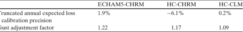
Table 1 Calibration precision of the annual expected loss and resulting gust adjustment factors

ECHAM5-CHRM HC-CHRM HC-CLM

Truncated annual expected loss 1.9% _−6.1% 0.2%

calibration precision

Gust adjustment factor 1.22 1.17 1.09

The AEL calibration method is chosen against several alternative pdf-calibration approaches, which have also been tested. These entailed using gust wind fields (not enough observational data), or the storm severity index (Lamb and Frydendahl1991) (no straightforward relation to loss or input gust field).

Now the selection criteria and calibration are applied to both CTL and A2 runs for the three RCMs and the expected loss changes in a warmer climate are determined.

4 Results

4.1 Control simulations

As prerequsite for the climate change impact study, an intercomparison of the base fields (mean wind gusts AVG, V98, mean gust of event days MGE) from the three different regional model runs nested into the two global climate models for present day conditions (CTL) is undertaken with Fig.6. These results (in particular

Figs. 6a, b) can also be related back to Fig.5, where CHRM has been driven by

the ERA40 reanalysis, which will be treated as representing “reality” for the current intercomparison. The plots show interesting similarities and differences and together provide an insight into the uncertainty range inherent to the various steps of the climate model chain.

The overall structure and patterns of both AVG and V98 (Fig.6; top and middle) are very similar for all simulations. In particular both CHRM climate simulations (Fig.6a, b; top) bear close comparison with the downscaled ERA40 data (Fig.5a). Hence it can be argued that the CTL runs are able to reflect satisfactorily the current climate gust conditions. A good correspondence between observed and simulated cyclone tracks and wind fields has similarly been reported in other studies using

the HadCM3/HadAM3 modeling chain (Leckebusch and Ulbrich2004; Rockel and

Woth2007; Pinto et al.2007).

However, noteworthy differences exist. Firstly, it is interesting to record that the gust fields differ significantly less between the two regional models (using the

same global model, Figs. 6b, c), than a single regional model (CHRM) driven by

different global models (Figs.6a, b). This confirms the importance of including the uncertainty related to different global climate models (GCMs) into nested regional impact studies.

Secondly, a closer look at the regional models driven by the same GCM (Figs. 6b, c) reveals only minor deviations over the oceans, but considerable dif-ferences over land, i.e. Spain, Great Britain, European continent. There, AVG and

V98 values in HC-CHRM are reduced by about 1–2m/s and 2–4m/s, respectively,

compared to HC-CLM. An exception is Scandinavia where values and structure remain more similar.

40 45 50 55 60 65 40 45 50 55 60 65 40 45 50 55 60 65 40 45 50 55 60 65 40 45 50 55 60 65 40 45 50 55 60 65 40 45 50 55 60 65 40 45 50 55 60 65 40 45 50 55 60 65 –20 –10 0 10 20 30 40 –20 –10 0 10 20 30 40 –20 –10 0 10 20 30 40 –20 –10 0 10 20 30 40 –20 –10 0 10 20 30 40 –20 –10 0 10 20 30 40 –20 –10 0 10 20 30 40 –20 –10 0 10 20 30 40 –20 –10 0 10 20 30 40 4 5 6 7 8 9 10 11 12 13 14 15 16 17 18 19 20 21 22 23 24 25 14 15 16 17 18 19 20 21 22 23 24 25 26 27 28 29 30 31 32 33 34 35 4 5 6 7 8 9 10 11 12 13 14 15 16 17 18 19 20 21 22 23 24 25 (a) (b) (c)

Fig. 6 Comparison of mean gust fields (top, AVG), local 98% quantiles (middle, V98) and mean

gust for all selected event days (bottom, MGE) for the three nested RCM CTL runs for Oct–Mar 1961–1990 (shaded, m/s, contour interval 1 m/s). a ECHAM5-CHRM, b HC-CHRM, c HC-CLM. Note that the contour values are 10 m/s larger for V98

Thirdly, further intercomparison of V98 over land shows that the CLM exceeds all

other model runs by 1–4m/s. In terms of V98 it is followed by the ECHAM5-CHRM,

ERA40-CHRM and then HC-CHRM. HC-CLM and to a lesser degree ECHAM5-CHRM also exhibit positive offsets over the land areas for AVG. Possible reasons are differences in the friction/roughness parametrizations, differences in storm tracks with the local wind maximum protruding farther into the Gulf of Biscay (CLM), and the generally stronger wind speeds particularly over the oceans (ECHAM5).

Fourthly, the local V98 maxima over the oceans (Baltic Sea, German bight, Mediterranean) are less intense (2m/s) in the HC-driven run (Fig.6b) than in both

the ECHAM5-CHRM (Fig.6a) and ERA40- CHRM (Fig.5).

From the above the following conclusions about the structure of the gust prob-ability distribution functions (pdf) can be drawn. Over water, the means of the

ECHAM5-CHRM and ERA40-CHRM wind pdfs are comparable, but underesti-mated by CLM and CHRM. Over land the mean is overestiunderesti-mated by HC-CLM and underestimated by HC-CHRM. These differences are more pronounced for the extremes of the pdf, where heavy tails are featured by ECHAM5-CHRM over the ocean, and by HC-CLM over land. HC-CHRM gust extremes fall off strongest, in particular over land areas.

Finally, the event gusts (MGE) are the relevant fields for the coupling to the insurance model (Fig.6, bottom row and Fig.5c). The losses and selection criteria are only calculated over land, and the resulting sample sizes underlying Fig.6amount to 335 (ECHAM5-CHRM), 308 (HC-CHRM) and 665 days (HCCLM). Note that the overall structure of the MVG field is similar to the AVG. More specifically, over land, ECHAM5-CHRM and HC-CLM show the highest MVG values and HC-CHRM the lowest (with the exception of Scandinavia and Great Britain). For completeness we

mention that over the ocean HC-CLM has weaker winds by 1–2m/s in comparison

to HC-CHRM, which itself is 2–4m/s less than ECHAM5- CHRM (storm track,

Baltic Sea).

The previous observations stress the advantage of applying the multi-model approach on all levels of the model hierarchy. They also point to the possibility of obtaining a sizeable range in damage results, since the largest spread between the regional models is observed over land.

4.2 Climate simulations (A2)

Before proceeding with the estimation of wind damages, we consider the changes

in the gust fields in a warmer climate (A2-CTL). Figure 7reveals the changes to

gust fields expected in the A2 scenario, for the 3 nested RCM simulations. Given the existing differences in the CTL gust fields (Section4.1) it is reassuring that the overall changes recorded in all model runs exhibit a consistent structure and amplitude range.

The climate change pattern that stands out most is the increase in gust speeds in a broad band stretching from the Atlantic, over Great Britain into Northern and Central Europe. The increase is felt strongest in the ECHAM5-CHRM, where it extends farthest to the east with a signal all the way to Eastern Europe. This area of gust increase is straddled by two adjacent bands of reduced gusts span-ning from the Northern Atlantic to Scandinavia, and from Spain to the Eastern Mediterranean Sea.

The maximum of the AVG increase is in the English channel and the German

bight (0.8–1.4m/s, corresponding to a 6–8% increase), and it is weaker (0.4–

0.8m/s, 3–7%) over the NW-European continent. The decrease over Iceland and Scandinavia is of a similar magnitude (−1.2m/s, ∼6%), while the impact over the

Mediterranean amounts to only half of that (−0.4m/s, ∼3%). The same change in

structure is predicted for V98, pointing to the fact that the entire gust-pdf will shift to higher values in a corridor across Western and Central Europe. The relative change at the tail of the distribution, however, is less than that of the mean, suggesting

changes in variance and/or skewness of the pdf. V98 values increase by 0.8m/s

(∼3%) near the channel, and decrease by 1.2m/s (∼4%) and 0.8m/s (∼3%) over

(a) 40 45 50 55 60 65 –20 –10 0 10 20 30 40 –20 –10 0 10 20 30 40 –20 –10 0 10 20 30 40 –20 –10 0 10 20 30 40 –20 –10 0 10 20 30 40 –20 –10 0 10 20 30 40 –20 –10 0 10 20 30 40 –20 –10 0 10 20 30 40 –20 –10 0 10 20 30 40 40 45 50 55 60 65 40 45 50 55 60 65 40 45 50 55 60 65 40 45 50 55 60 65 40 45 50 55 60 65 40 45 50 55 60 65 40 45 50 55 60 65 40 45 50 55 60 65 (b) (c) –2.2 –2 –1.8 –1.6 –1.4 –1.2 –1 –0.8 –0.6 –0.4 –0.2 0 0.2 0.4 0.6 0.8 1 1.2 1.4 1.6 1.8 2 –4.4 –4 –3.6 –3.2 –2.8 –2.4 –2 –1.6 –1.2 –0.8 –0.4 0 0.4 0.8 1.2 1.6 2 2.4 2.8 3.2 3.6 4 –2.2 –2 –1.8 –1.6 –1.4 –1.2 –1 –0.8 –0.6 –0.4 –0.2 0 0.2 0.4 0.6 0.8 1 1.2 1.4 1.6 1.8 2

Fig. 7 Climate change impact on winter gust fields. As for Fig.6, but shown is the difference between the A2 scenario (Oct–Mar 2071–2100) and CTL (Oct–Mar 1961–1990). Note the different contour values for each set (row) of figures. a ECHAM5-CHRM. b HC-CHRM. c HC-CLM

Applying the same selection criteria as for the CTL runs (v/V98_CTL>1.3) to

the A2 simulations yields an increase in the overall number of selected events in

a warmer climate.1 _{Hence in addition to the increase in the strength of the gusts}

recorded above, the frequency of the selected events appears to rise. However, there are large regional differences and these will be discussed in the next section. The spatial structure for MGE is again similar to the AVG and V98, and hence confirms that the selection criteria result in a useful reduction of the initial data set. Quantitatively, the MGE changes are larger than for AVG and V98: a 6–8%

(1–1.5m/s) increase over the English channel/German bight, and decreases of 8–10%

(1.5–2m/s) over Iceland/Scandinavia and ∼7% (1m/s) in the W-Mediterranean.

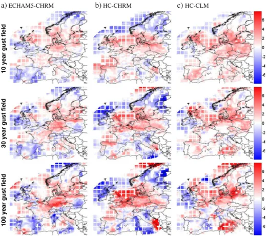
4.3 Changes in return periods

As outlined above (Sections2.2and3.1) we now step from one modeled event set

per climate run to the stochastic generation of a much larger, physically consistent, probabilistic event set that enables us to calculate wind fields for return periods much longer than the original 30-year integration period (cf. Section2.2).

Figure8shows the climate-change induced differences in gust amplitudes that can be expected for events with a return period of 10, 30 and 100 years, respectively. The three models show a high degree of consistency in both the spatial pattern and the amplitude range between the different time horizons. The patterns also relate closely to the gust field changes (AVG, V98) from Fig.7. However, the two figures show distinct information (mean wind field for all events vs. local wind speed for a particular return period) and should not be compared in detail. Note also that the fields in Figs. 7 and 8 are purely statistical information and bear no physical

a) ECHAM5-CHRM b) HC-CHRM c) HC-CLM

100 year gust field

30 year gust field

10 year gust field

Fig. 8 Climate change impact on storm gust fields for different return periods, (top) 10 years,

(middle) 30 years, (bottom) 100 years. Shown is the difference in event amplitude between the A2 scenario (Oct–Mar 2071–2100) and CTL (Oct–Mar 1961–1990) for the given return periods (shaded, m/s, contour value range is between_{+/− 8 m/s), based on the probabilitstic event sets. See text} for details. The data is represented on the irregular insurance model grid. a ECHAM5-CHRM.

meaning: i.e. the wind fields shown will in general not match any physically realised wind field in the data set. There are no obvious quantitative differences between the different model results (Fig.8a–c). Expected changes tend to be larger for the

rarer events (bottom panels) and amount to changes by up to about+/− 8m/s. The

consistent changes for the return periods comprise: -a decrease in event amplitude over Northern and Central Scandinavia, -a decrease over Ireland, -an increase over Southern Scandinavia, Northern Great Britain, the English channel and the North Sea, the Low countries, Germany (most dramatic over Northern Germany), and extending towards Poland and the Baltic States, -an increase over Southern Italy and the Adriatic Sea.

There is also some potential for an increase in extreme gusts over the Alps. Less certain and weak are the changes that occur over France, where an increase is projected for lower return periods, but the results are inconclusive for the higher return periods. Models are inconsistent over Southern Great Britain, where HC-CHRM shows an increase while the other two models predict a decrease. Similarly although rather strong signals are present over Spain, the results are contradictory and no conclusion can be drawn. An explanation for the latter shortcomings can be sought through the observations made earlier (Figs.6,7), which exhibit complex and non-conform model behavior over Spain.

4.4 Changes in losses—climate change impact

The generated probabilistic event sets are the input for Swiss Re’s insurance loss model, which is applied to the market portfolio (cf. Section2.2). The resulting climate change impact for insured winter storm losses is calculated with each of the three model chains and then evaluated in two complementary ways. First, the losses that occur in a particular frequency range (AEL, 10-year, 30-year, 100-year) for the entire

European portfolio are given in Table 2 and plotted in Fig. 9. This information

is subsequently regionalized by countries and shown for the AEL-level in Fig.10.

The error bars in these figures encompass the results of the three model chains considered.

From our analysis it can be seen that the area-mean impact is positive for all

frequency bands and models considered (Fig.9, Table2). For the annual expected

losses AEL, the results exhibit a mean increase of 44%, with an uncertainty range provided by the model ensemble between 16%–68%. For longer return periods the expected European-wide change increases non-linearly from 23% (10-years) to 50% (30-years) and to 104% for the 100-year loss. The change is least significant for the 10-year events. The associated model spread is particularly large for the rare events (53%–156%). In summary, the more infrequent an event, the greater the increase in expected loss. In economic terms, the loss increase is disproportionately large for the high layers. To illustrate the implications, consider the following numerical example

Table 2 Climate change

impact on the European market portfolio for the annual expected loss (AEL), the 10−, 30− and 100-year loss

Climate impact ECHAM5-CHRM HC-CHRM HC-CLM

1-year loss (AEL) 16% 68% 48%

10-year loss 3% 39% 25%

30-year loss 13% 93% 45%

Fig. 9 Mean climate change

impact on the European market portfolio for the annual expected loss (AEL), and the losses with return periods of 10−, 30− and 100-years. Uncertainty bars show the range of the three different coupled model outputs. See Table2for individual precentage values

WS climate impact

Annual expected loss and 10, 30 and 100-year loss for Europe

104% 50% 23% 44% 0% 40% 80% 120% 160%

Annual expected loss 10-year loss 30-year loss 100-year loss

Difference [% of CTL]

based on the mean values of the models used (Heck et al.2006). Currently, the AEL burden from winter storms in Europe is about EUR 2.6 billion. Assuming linear progression, this figure could increase by around EUR 11 million annually. At first glance, the rise may not seem all that dramatic, particularly since all models have some element of uncertainty, and natural variability will confuse the signal of the underlying trend. However, this means that if claims were to increase by EUR 110 million, or almost five percent of today’s levels within ten years, the expected annual insured loss from winter storms in Europe would be EUR 3.5 billion in 2085. That is EUR 0.9 billion more than at present. Similarly, for the highest layer in Fig.9, the current 100-year loss for Europe of EUR 21 billion, the results suggest an annual increase of almost EUR 200 million, leading to a rise of EUR 2 billion in ten years (a 10% increase compared to current loss levels).

The AEL for some of the national portfolios are summarized in Fig. 10. Most

European countries show a considerable increase in AEL, but the climate change

impacts differs from country to country (between−23% and +116%). Consistent

with our analysis in Figs.7and8, there is an expected reduction in AEL for Ireland, parts of Scandinavia and parts of the Mediterranean region. Large regional variations exist in the mean and the spread, such that the deviations from the European mean (Fig.9) can be substantial in individual countries. The highest impact is found for

Denmark and Germany (labeled DNK and DEU in Fig.10), which both are situated

within the band of strongest gust increase over the North Sea (cf. Figs. 7and 8).

Fig. 10 Regional climate

change impact on annual expected losses for selected regional market portfolios. Mean increases (red bars) and uncertainties (i.e. spread) of the three different coupled model results

WS climate impact Annual expected loss per country

-23% 16% 19% 35% 47% 67% 80% 95% 114% 116% 44% -50% 0% 50% 100% 150%

EUR DNK DEU SWE BEL NLD FRA GBR CHE NOR IRL

The models agree best for Germany, while for Denmark the spread is slightly higher. France shows the closest correspondence to the European mean, with a moderate spread. Larger uncertainties are found for Belgium and Sweden, but all models still predict an increase. In Great Britain the wind change has opposite signs for the northern and southern parts of the country in some models, but uniformly positive in others (cf. Section4.3and Fig.8), which explains the huge spread and renders the mean loss-increase non-significant. Finally, Switzerland, Norway and in particular Ireland show a potential for a reduced AEL climate change impact, i.e. a decrease in storm damage, but the results are still not conclusive.

A comparison with the spatial patterns of the return period wind fields (Fig.8) and the patterns of the frequency change of gust events (not shown) reveals close similarities, and hence it can be concluded that the observed climate change impact on the losses is a combined effect of changes in storm intensity as well as frequency.

5 Discussion

5.1 Comparison with previous studies

Wind gusts When comparing the wind gust fields simulated by similar coupled

GCM-RCM model chains, several interesting similarities and differences exist.

Consistent with previous publications (Leckebusch et al. 2006) we find a good

correspondence of the amplitudes and wind patterns of the RCM control runs with downscaled ERA40 data and observations. ECHAM5 (HC) only slightly

over-(under-)estimate the ERA40-CHRM gust speed (Figs.5,6).

Downscaling and the use of sophisticated gust parametrizations is instrumental in reproducing high gusts amplitudes, especially in the upper tail of the distribution

(Rockel and Woth2007). Compare for instance the∼50% increase (larger over land)

in gust amplitude of the 98% quantile between the ECHAM5 (Pinto et al. (2007),

their Fig.3c) and the CHRM gusts downscaled from the same global model (Fig.6a, 2nd row). In a comparable, but different GCM-RCM ensemble, Leckebusch et al.

(2006) find that the HC-CHRM, as their only model with a gust parametrization,

performs best in mimicking (even slightly overestimating) gust observations, espe-cially for the high quantiles.

Uncertainties introduced into RCM simulations by emission scenarios and bound-ary conditions have been found to exceed the variability between different RCMs (Leckebusch et al. 2006; Déqué et al.2007). Our results support these findings, a stronger variability of the wind fields with different GCMs is observed, than between different RCMs using the same global model (cf. Fig.6).

In terms of the gust changes predicted under the A2 scenario, the coherent picture emerges that the increase in gust frequency and amplitude is overproportionally large for the upper quantiles of the distribution. This is linked to an increased storm track of intense events over central Europe (southern UK, Northern Germany and Denmark) and decreased occurrence over the Mediterranean and Scandinavia. These areas are consistently found in both GCM and coupled GCM-RCM studies. Quantitatively, climate change signals for the 98% quantile of ECHAM5 winds

(Pinto et al. (2007), Fig. 5f–h) range between −1.2m/s and +0.9m/s, which is

probably due to the reasons mentioned above. A fairer comparison can be under-taken with Leckebusch et al. (2006), cf. their Figs.6and7, who find up 2–4% increase in the 99% quantile intensity and 25–50% increase in frequency with their set of

RCM-models. This corresponds very well to the∼3–5% increase in our simulations

for the 98% quantile intensity.

These results are also in line with the earlier studies mentioned in the introduction. However it should be noted that the uncertainties associated with rare events are still largely unknown, and the model spread could be strongly underestimated.

Insurance loss A quantitative comparison for the climate change impact on

insur-ance loss is hampered by the fact that projected insured losses derived from a coupled climate-damage model have not been published previously in the open literature.

A qualitative comparison can be undertaken with the loss potentials derived in

Pinto et al. (2007) and Leckebusch et al. (2007) for GCM wind gusts, which, as

mentioned before, estimate a wind-damage relation following Klawa and Ulbrich

(2003). Our results would correspond to their “no-adaptation” case under the A2

scenario, however, they consider changes for all events, whereas we use the proba-bilistic approach to estimate changes in different frequency layers, which makes the studies difficult to compare.

The general characteristics of the losses are similar to the ones stated for the wind, i.e. areas affected, largest changes for highest wind speeds (or rarest events, Figs.9,

10), hence qualitatively, the studies agree very well. The increased loss potentials are linked with enhanced values for the high percentiles of surface wind maxima over Western and Central Europe, which in turn are associated with an enhanced number and increased intensity of extreme cyclones over the British Isles and the North Sea (Pinto et al.2007).

Leckebusch et al. (2007) focus on loss potentials for Germany and the UK, and

their 4-member GCM ensemble yields an increase of+21% and +37%, respectively.

Although we cannot quantitatively compare the loss ratios due to different method-ologies, this is partly contrary to our results, where Germany accounts for much more future losses than the UK (cf. Fig.10). It is interesting that the inter-annual (not inter-model) variability range is much higher for the UK than for Germany, indicating a much broader loss distribution in the UK for the future climate (more extreme high- or low-loss events). Possibly, the larger inter-model variations for the UK-AEL in Fig.10is an expression of this. Also the disproportionate intensification of the minima and maxima for the rarer event gust fields could support that (Fig.8), and the projected zero-wind line cutting across the UK might be one reason for the large variability in the projections.

In Pinto et al. (2007) 3 different realisations of the same GCM (ECHAM5) are

used for the loss estimation, and applied to 4 different European regions. They estimate that the climate change impact on losses over the 100 years is largest for

Germany (+49%) and France (+44%), followed by the non-significant changes

observed for the UK (+24%), Sweden/Norway (+10%) and Portugal/Spain (−5%).

The order of our regional AEL is somewhat similar, but differs in that Sweden might experience quite a large increase, whereas there is no significant change detected for Norway. Pinto et al. (2007) also determine a significantly increased inter-annual variance for all the countries experiencing a loss increase, which corresponds to a reduction of return periods for extreme events, and this agrees well with our results.

In conclusion, it can be argued that although a direct comparison of absolute loss values is difficult, the tendency for the regional impact bears some similarity. More importantly, despite the completely different approaches, a consistent change to the loss distribution is projected under climate change, with increased variability at the upper tail, and an expected reduction of return periods for the countries affected by the shifting storm track.

5.2 Caveats and limitations

A primary prerequisite for this study was to achieve a dynamically meaningful coupling of the climate models with the insurance model, while applying the simplest-possible method. This is a very pragmatic approach which is likely to be prone to a number of shortcomings. Other caveats arise from assumptions and uncertainties associated with each step of the methodology. These limitations are discussed in detail below.

In this study a small ensemble of climate model simulations has been used, and it has become evident from our analysis that the application of a multi-model ensemble on all scales considered is vital to obtain an estimate of the model uncertainty and significance of the results. Global-to-regional model chains incorporate a number of errors and uncertainties, which together amount to the forecast uncertainty (e.g., IPCC2001; Schwierz et al.2006). In general these include: emission scenario uncer-tainties (not considered here), unceruncer-tainties arising from the chaotic nature of the coupled atmosphere/ocean system, imperfect knowledge of the initial and boundary conditions; and errors in the imperfect numerical representation of dynamical and physical processes. The multi-model ensemble considered in this study is very small, and it is likely that the uncertainties are considerably larger than suggested by the error bars provided. Indeed, the driving atmospheric GCMs produce rather similar circulation changes over the European continent, and consideration of all available GCMs would yield a larger spread. Nevertheless, it is worth pointing out that the two GCMs considered are among the best when evaluated regarding their ability to represent synoptic-scale circulation types under current climatic conditions (van

Ulden and van Oldenborgh2006).

Similarly it can be argued that additional RCMs should be included in the analysis, in order to better represent the downscaling uncertainties, in particular as we have to rely on parameterizations of wind gusts. Here problems arise from uncertainties in the formulations of turbulence and boundary layer processes, as well as from the limited spatial resolution available and the use of a smoothed representation of the surface topography. However, our choice has been objective in the sense that we have used all RCM simulations available that were equipped with an advanced gust parameterization. Furthermore, the similarity of the CLM and CHRM results (despite using two models with a completely different dynamical core—one being hydrostatic the other non-hydrostatic) suggests that the uncertainties on the GCM-scale dominate for the current application over those on the RCM-GCM-scale.

Although the performance of our straight-forward selection criterion for event-days has been critically and successfully tested with reanalysis data, there is potential room for improvement. We focussed on land-points and their selection depends on the accuracy and resolution of the land-sea mask. It would also be interesting to include sea points close to the coastline in a future extension of this model. A more