Mitigation of atmospheric perturbations and solid Earth movements in a TerraSAR-X time-series

DOI 10.1007/s00190-011-0515-6 O R I G I NA L A RT I C L E

Mitigation of atmospheric perturbations and solid Earth

movements in a TerraSAR-X time-series

Adrian Schubert · Michael Jehle · David Small · Erich Meier

Received: 12 May 2011 / Accepted: 5 September 2011 / Published online: 24 September 2011 © Springer-Verlag 2011

Abstract The TerraSAR-X (TSX) synthetic aperture radar (SAR) marks the recent emergence of a new generation of spaceborne radar sensors that can for the first time lay claim to localization accuracies in the sub-meter range. The TSX platform’s extremely high orbital stability and the sensor’s hardware timing accuracy combine to enable direct measure-ments of atmospheric refraction and solid Earth movemeasure-ments. By modeling these effects for individual TSX acquisitions, absolute pixel geolocation accuracy on the order of several centimeters can be achieved without need for even a single tiepoint. A 16-month time series of images was obtained over a fixed test site, making it possible to validate both an atmo-spheric refraction and a solid Earth tide model, while at the same time establishing the instrument’s long-term stability. These related goals were achieved by placing trihedral cor-ner reflectors (CRs) at the test site and estimating their phase centers with centimeter-level accuracy using differential GPS (DGPS). Oriented in pairs toward a given satellite track, the CRs could be seen as bright “points” in the images, provid-ing a geometric reference set. SAR images from the high-resolution spotlight (HS) mode were obtained in alternating ascending and descending orbit configurations. The high-est-resolution products were selected for their small sample dimensions, as positions can be more precisely determined. Based on the delivered product annotations, the CR image A. Schubert (

B

Remote Sensing Laboratories, University of Zurich, Zurich, Switzerland e-mail: [email protected] M. Jehle e-mail: [email protected] D. Small e-mail: [email protected] E. Meier e-mail: [email protected]

positions were predicted, and these predictions were com-pared with their measured image positions both before and after compensation for atmospheric refraction and systematic solid Earth deviations. It was possible to show that when the atmospheric distortion and Earth tides are taken into account, the TSX HS products have geolocation accuracies far exceed-ing the specified requirements. Furthermore, this accuracy was maintained for the duration of the 16-month test period. It could be demonstrated that with a correctly calibrated sen-sor, and after accounting for atmospheric and tidal effects, tiepoint-free geolocation is possible with TSX with an abso-lute product accuracy of about 5 cm.

Keywords Atmospheric path delay· Solid Earth tides · Geolocation accuracy· GPS · Plate tectonics ·

SAR geometry· TerraSAR-X

1 Introduction

A primary goal of any Earth-observing, remote sensing sys-tem is the ability to assign accurate geographic positions to the surface features being imaged. The degree to which it is able to do this is referred to as its geolocation accuracy. Until recently, image products from spaceborne synthetic aper-ture radar (SAR) sensors have all required time-consuming geometric pre-processing, usually involving operator inter-vention and the collection of ground control points (GCPs) and image tiepoints, before they could be layered with other information sources within geographic information systems. A SAR sensor with high geolocation accuracy greatly sim-plifies the task of combining multiple data takes with one another, not only simplifying their inter-comparison, but also dramatically speeding up applications such as near-real-time disaster mapping. Accurate geolocation also permits multiple

image products to be quickly combined or layered with other data sources such as digital elevation models (DEMs), cadas-tral maps, vegetation maps, forest maps, hydrological maps, etc. Finally, the high geolocation accuracy of TSX raises the possibility of its use as a geometric reference for other instru-ments (including optical sensors), where the sensor model is not as well known a priori. For example, this could be possi-ble through automatic feature matching based on one or more TSX images and an optical image dataset to be rectified; this technique was already demonstrated byReinartz et al.(2011) to be feasible.

Recently, the spaceborne SAR system TerraSAR-X (TSX) has begun to provide data with unprecedented geolocation accuracy. TSX is a German Earth observation satellite, built in the context of a public–private partnership between the German Federal Ministry of Education and Research (Bun-desministerisum für Bildung und Forschung; BMBF), the German Aerospace Center (Deutsches Zentrum für Luft- und Raumfahrt; DLR) and Astrium GmbH. The launch took place on 15 June 2007, and the sensor has a nominal lifetime of 5 years, although it is currently expected to last up to 7 years. The payload of the satellite is an X-band SAR system with a 9.65 GHz center frequency, an electronically steerable phased-array antenna and a side-looking imaging capability within an off-nadir pivoting range of approximately 20◦–55◦. The satellite is in a near-polar dawn/dusk orbit at an altitude of 514 km. Using its active radar antenna, it is able to produce image data with a spatial resolution on the order of∼1 m, regardless of weather conditions, cloud cover or absence of daylight.

A SAR sensor mounted on an air- or spaceborne plat-form measures target positions along two dimensions: its distance from the sensor, or range and its along-track posi-tion or azimuth. These two dimensions are inherent to a SAR measurement and are reflected in the format of the image products generated, called slant-range images. The ranging and azimuth timing measurements are independent of each other and thus contribute separately to the sensor’s total 3-D geolocation accuracy. While the high geolocation accuracy of the TSX products has already been partially dem-onstrated (Eineder et al. 2011;Schubert et al. 2010;Weydahl

and Eldhuset 2010;Ager and Bresnahan 2009;Jehle et al.

2008;Nonaka et al. 2008;Schubert et al. 2008), all previous

studies were partially hindered by one or more uncertain-ties that have been eliminated in the present study.Eineder

et al.(2011) demonstrated that absolute ranging accuracy is

better than 10 cm for a correctly calibrated instrument, and they measured relative accuracies as high as∼3–6 cm. How-ever, the along-track (azimuth) geolocation accuracy was not measured in the study. The remaining studies were hindered either by artifacts related to the GPS reference frame, mea-surement uncertainties or insufficient accounting for one or more perturbations acting upon the SAR signals, such as the

solid Earth tide (SET). Finally, the long-term stability of the sensor’s localization accuracy had not yet been established firmly; this is treated in this study.

The sensor’s high product geolocation accuracy can only be achieved by modeling and correcting for the phenom-ena that measurably disturb the observed target positions. The refraction of electromagnetic waves in the atmosphere is the largest of these effects, typically causing range delays between 2 and 3 m at X-band. SET perturbations, caused by lunar and solar tidal forces acting on the planet as a whole, are the second-largest error source. They can cause verti-cal displacements of up to half a meter (peak-to-peak) at the equator (Melchior 1974;Milbert 2011), but typically no more than∼40 cm at mid-latitudes. An even smaller effect also exists: Earth deformation by ocean tide loading. As the oceans are periodically redistributed by the relative positions of the sun–moon–Earth system, the changing weight distri-bution of the water mass on the ocean bed causes the Earth to deform. These vertical fluctuations usually do not exceed several centimeters for inland sites (Penna et al. 2008) and are neglected in this study.

While the atmospheric and solid Earth perturbations can-not be separated in the SAR signal, modeling the effects indi-vidually for the particular acquisition geometry and test site permits indirect model validation. The problem can be stated as follows: if it is possible to accurately predict the location of a reference target in a SAR image having an accurately known position, then the imaging process has been repro-duced acceptably in the model-based corrections. As atmo-spheric and solid Earth movements influence the imaging process, an accurate prediction implies that our understand-ing of the processes involved is equally accurate. Conversely, incorrectly modeling the perturbations will prevent accurate geolocation predictions. This study demonstrates the accu-racy and stability of the TSX system, as well as the validity of the atmospheric and physical models used, to within several centimeters of remaining uncertainty.

2 Experimental design

The primary goal of this study was to jointly validate the long-term stability of the TSX sensor and the Earth-system models used to adjust the SAR geolocation measurements. The test site was selected to meet the following criteria: (1) the cor-ner reflectors (CRs) placed there would have to remain stable and undisturbed for the duration of the 16-month test period (security), (2) it would need to be near permanent meteoro-logical and permanent GPS stations and (3) a concrete site would be preferred, to ensure a relatively dark background for the imaged reflectors, permitting accurate estimation of their phase center locations with subpixel accuracy. A test site was selected in the west of Switzerland near the village

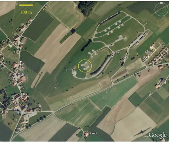
Fig. 1 Aerial view of test site

Torny-Le-Grand, Switzerland

of Torny-Le-Grand, which met all of the above criteria. Four trihedral CRs were placed at the site, with two permanently facing the TSX sensor perpendicular to its ascending-orbit and two facing its descending orbit. The site was imaged using TSX’s highest-resolution spotlight (HS) mode; this time-series of images provided the primary data basis for this study.

2.1 Test site and corner reflectors

The test site is nestled in Switzerland’s hilly midlands close to the city of Fribourg. Just outside of the village of Torny-Le-Grand, a former missile launch site of the Swiss Air Force served as an ideal location to place trihedral CRs for the dura-tion of the study. Four CRs were placed about 30 m apart from each other, each surrounded on all sides by enough concrete to guarantee good contrast in the SAR images. The site is shown in Fig.1, with the four round lots indicated with a yellow circle; a CR was placed in the center of each lot.

A permanent GPS reference station of the Automated GNSS Network of Switzerland (AGNES), located<5 km from the site near the town of Payerne, was used for the differential positioning. Trimble 5700 and Trimble R7 GPS receivers (Fig.2a) were used to measure their locations with accuracies better than∼1 cm, as given by the RMS reported by the receivers (this accuracy is confirmed byTrimble 2011).

The measurements were repeated midway through and at the end of the campaign to validate the positions used. Exist-ing mountExist-ing holes were used as the survey points. Each CR was then mounted such that its phase center (vertex) was in vertical alignment with the survey point (Fig. 2b). The vertical offset between the vertex and survey point was measured, providing an estimated overall absolute accuracy of∼1–2 cm, taking into account all the measurement error sources.

Two of the CRs are seen in Fig. 2c, oriented to face the satellite pass perpendicular to its orbit (i.e. towards the nearest approach). The two western-most CRs were oriented towards the ascending orbit with an elevation angle of 44◦; the two eastern-most faced the descending orbit with an ele-vation of 65◦. The ascending and descending geometries cor-responded to “long” (∼710 km) and “short” (∼561 km) paths through the atmosphere, respectively. Their appearance in an HS product (acquired on 25.08.2010) is shown in Fig. 2d. The CR sides have a length of 90 cm. A CR’s vertex is its phase center, the point from which the maximum amount of energy is reflected. Its location is given by the peak inten-sity in the center of the “cross” pattern in a radar image. The cross pattern (actually a sinc-like function in the range and azimuth dimensions, caused by constructive and destruc-tive interference of the coherent waves) is the characteristic point target response for a SAR (see section 2.8 in

Fig. 2 Surveying positions of the CRs. a GPS receiver over a mounting hole, b vertex alignment over the mounting hole, c CRs oriented towards the

descending orbit, and d CRs as they appear in an ascending HS product (range spacing 45 cm, azimuth spacing 87 cm; acquisition date 25.08.2010)

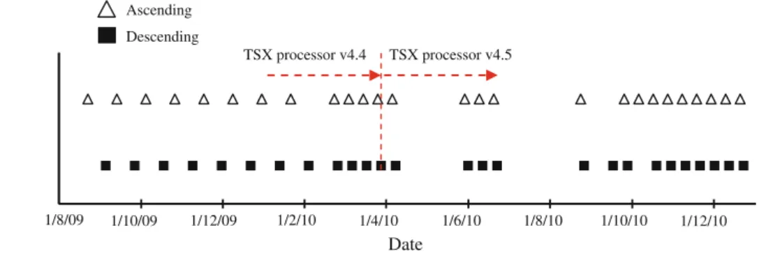
Fig. 3 TSX acquisition time

series over Torny-Le-Grand test site 1/8/09 1/10/09 1/12/09 1/2/10 1/4/10 1/6/10 1/8/10 1/10/10 1/12/10 Ascending Descending Date TSX processor v4.4 TSX processor v4.5

as calibration targets is available in section 10-3.3 ofUlaby

et al.(1982).

2.2 Time series

The satellite acquires image lines as it advances along its orbit, sending radar echoes down to Earth to the right, rela-tive to the platform’s path. A limited number of beams, corre-sponding to specific elevation angles or look directions, can be selected for imaging. This configuration led to a choice of one particular geometry for ascending orbits and another for descending orbits. The theoretical interval between two

identically configured (repeat-pass) acquisitions is 11 days. The observation period for this experiment was from August 2009 to December 2010. Within this time frame, 52 acquisi-tions were obtained in total. Of these, 26 were from ascending orbits and 26 from descending orbits. The product acquisition dates are shown graphically in Fig.3. The series represents a relatively continuous set of observations in a given mode over a fixed test site. Note that at the end of March 2010, the TSX processor was updated with new radiometric and geomet-ric calibration constants and methodologies. The 27 March 2010 acquisition was the first to be processed using the new version of the software. The effect of the recalibration was

clearly evident in our geolocation experiment, manifesting itself as a distinct improvement in the absolute geolocation accuracy.

2.3 Comparison between imaged and measured corner reflector positions

At the core of the test for geolocation accuracy is a compari-son between the surveyed location of a CR and its measured location in a SAR image. Given the radar timing annota-tions (time of first range sample, range sampling rate, first azimuth time, azimuth sample interval) and the state vectors describing the satellite’s trajectory during the time of data acquisition, a point on the Earth’s surface may be located within the image by solving the Doppler equation governing the image product’s geometry. This involves searching for the azimuth time where the satellite’s position corresponds to the required Doppler value. This geolocation method is called “range-Doppler” (Meier et al. 1993).

TSX’s HS images, with their sub-meter sample spacing, provide a good opportunity to precisely locate reflector peak returns. Reflectors were placed on concrete surfaces to min-imize clutter and allow precise location estimates. Apply-ing complex FFT oversamplApply-ing with a factor of 50 within a 128× 128 analysis window centered on a given reflector, its location is determined as the local intensity maximum with a precision of 1/50th of a sample (Small et al. 2004a). The slant range from the sensor to the reflector can then be obtained using the range timing annotations.

The surveyed locations of the CRs were predicted within the radar image products. Additional corrections were made for perturbations described in the following sections, as well as a constant azimuth timing shift indicated in the product annotations for the geolocation grid. The latter provided in the TSX product annotations (Fritz 2007), claims to take “rel-ativistic Doppler” and “internal timing effects” into account. The predicted coordinates were then compared with the cor-responding measured positions, yielding a single estimate of the geolocation accuracy. This is illustrated in Fig.4for the two reflectors facing the ascending orbit. For each CR, its predicted location is marked with a blue cross, the result of transforming the differential GPS (DGPS) coordinate of the CR phase center into slant-range image coordinates. The zoom level increases towards the bottom.

During the estimation of the imaged CR position, a quality indicator is generated at the same time, the signal-to-clutter ratio SCR (Small et al. 2004b). This is defined as the ratio between the CR peak intensity and the mean surrounding intensity (excluding the “arms of the cross” caused by the side-lobes of the CR response). In practice, the mean back-ground intensity is calculated for the four quadrants created by the “cross” pattern, but well outside of the “arms” of the cross. As the SCR is a linear ratio, the radiometric calibration

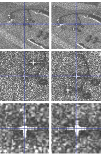
Fig. 4 Both ascending-orbit corner reflectors as seen in a slant-range

image, at three zoom levels. The crosshairs represent predicted loca-tions based on corner reflector DGPS measurements. Acquisition date 16.08.2009

of the samples is irrelevant. The SCR can be used to automate detection of unreliable measurements, as will be seen later.

3 Perturbations

In the absence of an atmosphere, tectonic plate movements and tidal effects, position measurements of stable targets on the Earth’s surface using SAR would be predictable and vir-tually unchanging from day to day. In reality, the sub-met-ric geolocation accuracy of TSX can only be achieved if proper account is taken of the effects acting on the radar echoes, which alter their measured arrival times at sensor level. The largest contributor to variable deviations in echo return time is atmospheric refraction. The SET cannot be neglected either, but it becomes critical only when an accu-racy of 1–2 dm or better is required. Finally, although it does not influence the geolocation accuracy of TSX per se, esti-mates of its accuracy using CRs and GPS may be signifi-cantly influenced by plate tectonics due to the use of different

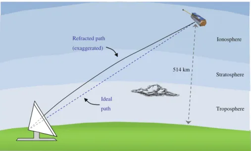
Fig. 5 Atmospheric path delay

(atmospheric layers not to scale, refracted path exaggerated)

Troposphere Stratosphere Ionosphere 514 km Refracted path (exaggerated) Ideal path

reference frames. These perturbations were all modeled and removed from our measurements; we were able to show that their removal resulted in very good agreement between the-ory and measurements. The effects are described in more detail in the following sections.

3.1 Atmospheric path delay

The TSX imaging geometry leads to a path length from sen-sor to ground of between∼550–730 km, traversing much of the ionosphere and the entire stratosphere and troposphere. The radar echoes travel more slowly in a medium than in a vacuum (this is why refraction occurs), contributing signif-icantly to the total travel time. This increase in the “ideal” travel time is called the path delay (PD). The situation is represented in Fig.5; the slowing effect of the atmosphere causes the radar echoes to deviate slightly from a straight path, additionally increasing the total traveled distance and hence traveled time. However, the additional delay caused by the path-length increase is negligible compared with the slowing effect itself (Jehle 2009). Pressure, humidity and temperature changes in the troposphere (the lowest∼11 km of the atmosphere) are the primary cause of refraction at X-band (Jehle 2009;Klawitter 2000), contributing typically ∼50 times more than the ionosphere to the total delay. The stratosphere contributes only a negligible amount. The tro-pospheric delay is composed of the hydrostatic delay (asso-ciated with the “dry” troposphere) and the wet delay. The modeled hydrostatic component can be considered accurate on the order of∼1 mm (Bevis et al. 1996), while the wet com-ponent is associated with a higher uncertainty of maximum ∼5 cm, according to calculations made during the prepa-ration of Jehle et al. (2008) (the “wet” component, when modeled using the method employed here, deviates from

ref-erence values—generated by a millimeter-accurate ray-trac-ing model—with a standard deviation of∼4.5 cm). It should be added that the model input parameters pressure, tempera-ture and humidity all influence the path delay uncertainty; the values stated above are valid for measurements made by the national weather service at a station near the imaged location, within a couple of hours of its acquisition).

The TSX product annotations include an approximate PD value, calculated using a simple atmospheric model that takes only the mean imaged terrain height and the viewing geom-etry into account (Fritz et al. 2008a). The model neglects real day-to-day atmospheric variations. While the annotated PD estimate yields much better range estimates than without their inclusion, they may nonetheless deviate from the true PD by approximately half a meter in the case of shallower viewing angles.

The atmospheric model used in this study to generate improved PD estimates is described inJehle et al.(2008) and

Collins and Langley(1996). It is a purely height-dependent

model calibrated using ground-based measurements of the air pressure, temperature and water vapor. For each individual data take, the meteorological measurements were obtained from the weather station Payerne, about 6 km north of the test site. Given these values, and under the assumption of a “mean atmosphere” for mid-latitudes, the PD was calculated for each individual TSX data set and illumination geometry. This estimate, independent of the radar data, was then used to adjust the range timing values, effectively “removing” the PD from the range measurements.

3.2 GPS reference frame drift

The tests of geolocation accuracy are based on compari-sons between imaged CR positions and their surveyed DGPS

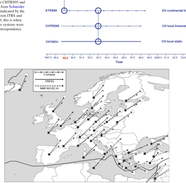
Fig. 6 Relationship between

the Swiss local geodetic reference system CHTRS95 and ITRS (modified fromSchneider

et al. 2001). As indicated by the

connection between ITRS and ETRS89 in 1989, this is when the two reference systems were last in perfect correspondence

Fig. 7 Velocities of European reference stations within ITRS (fromSchneider et al. 2001)

positions. The comparison carries with it the assumption that the geodetic reference frames defined for the satel-lite positions and the CR positions are identical. In fact, this is often not the case. The reference frame used for the orbit state vectors is WGS84-G1150 (an instantiation of the World Geodetic System defined by the National Imagery and Mapping Agency,NIMA 2004) according to the TSX prod-uct annotations (format described inFritz 2007). WGS84-G1150 and the International Terrestrial Reference Frame (ITRF) are identical to within approximately several cen-timeters at most, according toNIMA(2004) andSchneider

et al.(2001) (although no documentation of the relationship

is known to be publicly available). DGPS measurements of the CRs were provided in the Swiss Terrestrial Reference Frame CHTRF95, which is tied closely to the European

Terrestrial Reference System ETRS89 and is identical to it at the epoch 1993.0. Both are coupled to the stable part of the Eurasian continental plate. ETRS89, in turn, was defined in 1989 as identical to ITRS. Since 1989, these two frames have been slowly drifting apart due to their connections to dif-ferent continental plates. Figure6illustrates the relationship between the reference systems. The transformations between the ITRS/ETRS/CHTRS systems are documented, for exam-ple inSwisstopo(2006) andBoucher and Altamimi(2001). The relative drift within ITRS is shown in Fig.7, where Swit-zerland can be seen to be moving towards the north-east at a rate of∼2.5 cm/year. More precisely, the NNR–NUVEL1A model yields a motion of the Eurasian plate of 2.44 cm/year (calculated for example according to Deutsches

a 90% confidence interval estimated empirically as better than 0.3 cm/year byLarson et al.(1997). The Eurasian plate movement was modeled using the NNR–NUVEL1A kine-matic model (a version of the NUVEL1A model with “no net rotation”, or NNR), defined inDeMets et al.(1994). Thus, the total drift of CHTRS95 relative to ITRS between 1989 and the TSX acquisition period is∼50 cm.

By modeling the relative drift between CHTRS95 and ITRS for a given product acquisition date and projecting the movement into slant range and azimuth coordinates, the sur-veyed DGPS coordinates were transformed into ITRS. This was a necessary step for the subsequent geolocation tests and was found to be the primary source of residual errors in our previous study (Schubert et al. 2010), particularly in the along-track direction.

3.3 Solid Earth tide

Periodic deformations of the Earth cause vertical peak-to-peak fluctuations of up to∼40 cm at mid-latitudes. Relative to the tide-free state, this figure translates to SAR slant-range deviations of up to∼15 cm (i.e. ∼30 cm peak-to-peak) and much smaller horizontal displacements of a few centime-ter in the azimuth dimension. The SET model used is based on a computer program byMilbert(2011), an implementa-tion of the model described inMcCarthy and Petit(2004). The authors state the model to be accurate to∼1 mm. We compared the model calculations with the results of another model with a claimed accuracy of∼1 cm and observed agree-ment at the centimeter level, thus validating the tidal model used here to at least∼1 cm accuracy.

The tidal movement in 3-D of a single CR is shown for a full day (24.12.2010) in Fig.8. Part (a) shows the move-ment separated into its vertical, north and east components, while (b) shows the same movement viewed from above. The dominant component is vertical, with a maximum devi-ation of about 16 cm shortly before 09:00 UTC. However, the acquisition on 24.12.2010 was at 17:25 UTC, when the ver-tical deviation was only∼12.2 cm; this translates to ∼9 cm in the slant range direction for the corresponding ascending geometry.

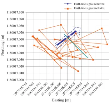
In Fig.9, the horizontal map positions (easting and north-ing) of one CR at the test site are plotted for the entire test period. The noisy orange data series includes all solid Earth effects, reflecting the irregular horizontal motion of the Earth’s surface under the influence of the moon and sun. The blue series is obtained after removal of the modeled SET. It begins at the bottom left on 16.08.2009 and progresses in time towards the north-east. What remains is the movement of the CHTRF95 coordinates within the global ITRF reference frame due to plate tectonics; it is equivalent to the dotted arrow extending from Switzerland in Fig.7. The total dis-tance traveled over the test period of 484 days was 3.36 cm,

Time of day (UTC)

Earth tide [m] (a) -0.20 -0.15 -0.10 -0.05 0.00 0.05 0.10 0.15 0.20 0.25 12:00:00 AM 2:00:00 AM 4:00:00 AM 6:00:00 AM 8:00:00 AM 10:00:00 AM 12:00:00 P M 2:00:00 P M 4:00:00 P M 6:00:00 P M 8:00:00 P M 10:00:00 P M 12:00:00 AM

Earth Tide Vertical [m] Earth Tide East [m] Earth Tide North [m]

(b) -0.07 -0.06 -0.05 -0.04 -0.03 -0.02 -0.01 0.00 0.01 0.02 0.03 0.04 0.05 0.06 0.07 -0.07 -0.06 -0.05 -0.04 -0.03 -0.02 -0.01 0 0.01 0.02 0.03 0.04 0.05 0.06 0.07 Northin g [m] Easting [m]

Fig. 8 Motion of a CR due to solid Earth tides over a 24-h period on

24.12.2010. a Variation of vertical, easting, and northing components of motion, and b easting and northing components of motion, top view

Northin g [m] 118 118 118 118 118 118 118 118 118 118 118 001 001 001 001 001 001 001 001 001 001 001 7.00 7.01 7.02 7.03 7.04 7.05 7.06 7.07 7.08 7.09 7.10 00 10 20 30 40 50 60 70 80 90 00 Easting [m]

Earth tide signal removed Earth tide signal included

Fig. 9 Decimeter-scale horizontal motion of a GPS receiver over the

16-month study period. The orange points are affected by Earth tides as well as plate movement, while the blue points have had Earth tides removed, isolating the north-east drift of the Eurasian plate relative to the ITRS frame

corresponding to a 2.53 cm/year drift rate and a heading of 36.5◦. The drift rate is well within the 90% confidence inter-val for the NNR–NUVEL1A plate model (see the previous section). Its heading is 36.5◦, which compares very well to the 34.9◦heading produced by the NNR–NUVEL1A model. We can therefore conclude that the observed drift is mainly due to the relative drift of the local and international reference frames.

4 Results

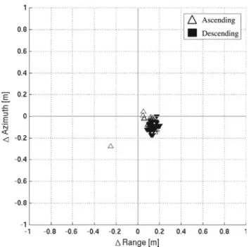
The core of the geolocation accuracy tests consists of a comparison between the imaged CR locations and their pre-dicted positions, as described in Sect.2.3. Four sets of test results are presented in the following sections, each subse-quent result set incorporating an additional corrective mea-sure. The results are presented in a scatter plot format, where the difference between the predicted and measured range and azimuth coordinates is plotted for each CR and each product. Two data points therefore exist for each TSX product. Dif-ferent symbols distinguish ascending- from descending-orbit acquisitions. This distinction makes azimuth effects easily visible, as azimuth shifts have different signs for ascending and descending orbits. “Perfect” geolocation would result in range and azimuth differences of zero, which is at the center of the scatter plots in Figs.10,11and12. These plots extend from−1 to +1 m in both dimensions to simplify direct com-parisons.

Fig. 10 Offsets between measured and predicted corner reflector

posi-tions using delivered product annotaposi-tions (“out-of-the-box” test). Cor-rections applied: constant total atmospheric path delay delivered with the product annotations used to adjust radar timing

Fig. 11 Offsets between measured and predicted corner reflector

posi-tions. Corrections applied: constant path delay estimated by site- and time-specific atmospheric modeling, used to adjust radar timing

Fig. 12 Offsets between measured and predicted corner reflector

posi-tions. Additional correction applied: DGPS positions translated from their native CHTRS reference frame into the ITRS frame. The outlying point is from a partially snow-filled CR and can be discarded

4.1 “Out-of-the-box” accuracy

Many users of TSX image products will not be able to make the model-based corrections (PD and SET). Users not requir-ing better than ∼0.5 m accuracy do not need to be con-cerned with these corrections. However, to achieve∼0.5 m

geolocation accuracy, one correction must be applied at min-imum: the PD supplied in the delivered annotations should be subtracted from the range timing values. Applying that cor-rection before geolocation tests resulted in the error scatter plot shown in Fig.10. It is called the “out-of-the-box” result because of its sole dependence on the delivered annotations. Several points are worth noting about this result:

• The DGPS coordinates have not yet been projected into the ITRS; the separation between the ascending and descending point clouds is therefore not indicative of a geolocation error in the products themselves, but a mea-surement artifact (which will be corrected in a subsequent step).

• For reasons that will be discussed in Sect.4.6, only prod-ucts that were processed using version 4.5 (denoted v4.5) of the TSX processor are shown. This includes all prod-ucts delivered on 27.03.2010 and later, as well as six earlier acquisitions that were later reprocessed using the newer version.

4.2 Correction for atmospheric path delay

The “out-of-the-box” test made use of the nominal PD, which is not linked to the true local weather conditions that existed at acquisition time. Replacing the nominal PD with a more refined model (see Sect.3.1) results in a new error scatter plot, shown in Fig.11. As the PD is purely a range effect, the data points have been shifted along the horizontal (range) axis compared with Fig.10. The two main ascending and descending point clouds are now centered approximately on (0, 0).

4.3 Correction for GPS reference frame drift

The most dramatic improvement to the geolocation tests arises when the GPS coordinates are transformed into the ITRS reference frame before the CR predictions are made, in effect accounting for plate tectonics. Figure12shows the new scatter plot. In comparison to Fig.11, the ascending and descending point clouds have merged, with a mean error now visibly smaller than 20 cm in both dimensions.

A notable outlier can be seen in Fig.12 to the left of the main error cloud. The corresponding CR was from an ascending product from 02.12.2010. Heavy snowfall was observed the day before, confirmed by meteorological reports (from the Federal Office of Meteorology and Climatology, MeteoSwiss), with 10–20 cm of accumulation. It is therefore very likely that one or both of the CRs were partially filled with snow, altering the CR’s backscattering characteristics. In addition to this, the X-band radiation is partially scattered by snow, lowering the contrast between the CR backscatter and the surrounding snow-covered concrete. The difference

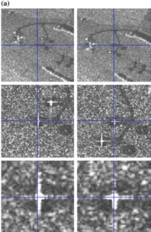
between a summer acquisition and the 02.12.2010 acqui-sition can be seen in Fig. 13. The snow-free reference is Fig.13a; part (b) is the same extract from the 02.12.2010 product. Although both CRs are visible in Fig. 13b, they are less distinct; the arms of the “cross” shape have disap-peared. Also, the backscatter from the surrounding back-ground (clutter) has increased due to the snow cover. The outlying error estimate in Fig.12corresponds to the right-most CR in Fig.13b, whose predicted position is visibly off-set from the center of the CR. We conclude that for this CR, the maximum backscatter does not correspond to its vertex position. This hypothesis is supported by the extremely low SCR of 9.3, which is∼20 times lower than for CRs in the other ascending products. We are, therefore, confident that this point can be discarded.

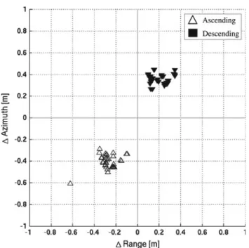
4.4 Correction for SET

The final correction applied to the CR positions is the cor-rection for the SET. As seen in Sect.3.3, the fluctuations are generally on the order of several centimeters, and they can be easily modeled and projected into the range and azimuth dimensions. Applying the corrections for SET perturbations, the error points converge even further; the result is shown in Fig.14.

At this point, all major corrections have been made to the CR positions. Discounting possible residual errors inher-ent within the atmospheric and tidal models themselves, the remaining offsets must be due to a combination of mea-surement errors, centimeter-level effects (such as ocean tide loading), minor geometric calibration errors and residual uncertainties in the orbital state vectors. Excluding the outlier (snow-filled CR), the mean range error is +13 cm with a stan-dard deviation of 3.3 cm; the azimuth error is−8.3 ± 4.4 cm. Given the various remaining error sources (the measurement of the CR phase center alone cannot be claimed to be more accurate than∼1–2 cm), this represents a remarkably high sensitivity and calibration precision for a spaceborne SAR sensor.

The 3.3 cm standard deviation value in range is consistent with the observed ranging spreads of 2.6–5.9 cm estimated

byEineder et al.(2011) in a similar study (which also

cor-rected for solid Earth tidal movements). Given the previously cited uncertainties associated with the atmospheric, tidal and tectonic models (∼5, ∼0.3 and ∼1 cm, respectively), it is remarkable that the total standard deviations in both dimen-sions of the corrected offsets is not>3–4 cm. Separating the dimensions: since the range spread should mainly be affected by path delay modeling errors, the∼3 cm standard deviation can be considered very small. The centimeter-level uncer-tainty in the solid Earth model results imply that the∼4 cm spread in azimuth is mainly due to orbital and timing errors augmented by solid Earth modeling errors.

Fig. 13 Comparison of CR detection in snow-free and snow-covered

scenes from the ascending orbit. The crosshairs represent predicted locations of the CRs. a Snow-free reference from 25.08.2010; SCR

(left) = 199.1, SCR (right) = 212.3. b Image from 02.12.2010 acquired after heavy snowfall; SCR (left) = 29.3, SCR (right) = 9.3

The error cloud is so compact that its offset from (0, 0) is probably due to a slight miscalibration of the sensor’s timing constants. Since this is a simple matter of processor (soft-ware) calibration, it is not a flaw in the sensor design itself. 4.5 Further investigations: signal-to-clutter ratio, seasonal

dependence and SAR processor version

Figure14was investigated further for significant correlation with the SCR (reliability of the imaged CR position) and time of year (seasonal reliability of the atmospheric model used to estimate PD).

To approach these two questions simultaneously, we plot-ted Fig.14again, encoding the SCR and seasonal information by varying marker color and size, respectively. The result is shown in Fig.15a: SCR is color-coded with the marker size indicating one of three seasonal groups. Figure15b is the same as (a), except that all points with SCR<150 have been eliminated. Based on these plots, we conclude that

1. no significant correlation between season and the accu-racy of the modeled PD is evident;

2. while extremely low SCR (i.e. <50) may occasionally indicate a false measurement of the CR location, the CR image analysis is usually robust enough to provide the correct location.

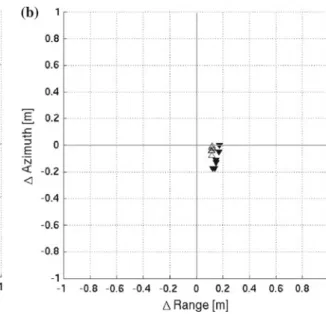
Concerning the processor version, the series of scat-ter plots presented in Sect. 4.1–4.5did not include many products processed prior to 27.03.2010. This is because a newly calibrated TSX processor was used from that point onwards, v4.5. A comparison between error plots for v4.4 and v4.5 for six acquisitions processed twice, once for each processor version, is given in Fig. 16. Part (a) shows the v4.4 plot, (b) the v4.5 plot. Both scat-ter plots include correction for PD, plate tectonics and the SET, so they are directly comparable to Fig. 14. The improved v4.5 azimuth and range calibration is clearly evident.

In summary, the scatter plot obtained in Fig.15a therefore represents our best estimate of the “inherent” TSX geoloca-tion accuracy at the time of this writing. It testifies not only to TSX’s extremely high geolocation accuracy, but also its long-term stability.

Fig. 14 Offsets between measured and predicted corner reflector

posi-tions. Additional correction applied: compensated local movements caused by solid Earth tides. The outlier to the left of the point cloud can be discarded as the reflector was partially snow-filled on that date, interfering with its nominal reflectance properties

4.6 Summary of geolocation accuracy estimates

The mean and standard deviation of the error scatter plots are listed in Table1. The best estimate of TSX’s current geolo-cation accuracy is italicized at the bottom of the table: under “typical” viewing conditions, the consistency (i.e. standard deviation) of the geolocation can be said to be within 3– 4 cm, while the absolute location accuracy is on the order of a decimeter. The absolute accuracy could be improved by a further adjustment of the TSX processor’s calibration con-stants, although it is already far below the 1-m requirement defined for TSX (Fritz and Eineder 2008b).

5 Conclusion

In this study, we acquired a 16-month time-series of high-resolution spotlight images from the TSX sensor over a test site in Switzerland. Four trihedral CRs were deployed and their positions were surveyed with approximately centimeter accuracy. We compared the measured CR positions with their imaged positions, based on the delivered product annota-tions and correcannota-tions made for atmospheric path delay, plate tectonics and SETs. The resulting error distribution is very compact and allows us to assign the TSX system an absolute geolocation accuracy of approximately 13 cm in range and 7 cm in azimuth, with a standard deviation of 3–4 cm in both dimensions.

Fig. 15 Offsets between measured and predicted corner reflector

posi-tions, color-coded according to the image signal-to-clutter ratio, and marker sizes according to season. Large triangles are from winter acqui-sitions, medium triangles from spring and autumn, and small triangles from summer acquisitions. a Errors for all products and b errors after removal of points with SCR<150

The sensor has proven to be sensitive enough to (incoher-ently) detect solid Earth movements on the order of several centimeters. At the same time, this study provided indi-rect evidence for the validity of the path delay and solid Earth tidal and tectonic models used during the study. Fur-ther work would be necessary to validate the models used in non-temperate latitudes, e.g. high arctic and equatorial regions.

Due to ever-improving data availability from Earth-obser-vation platforms, there is a current push towards an increased utilization of image time-series from one or more sensors. TSX has set a new geolocation standard for spaceborne SAR systems. However, this accuracy would be severely compro-mised were the atmospheric path delay not systematically mitigated. Therefore, we highly recommend the widespread inclusion of an atmospheric model in the product annota-tions, calibrated for the acquired scene by taking the best

Fig. 16 Comparison of offsets between measured and predicted corner

reflector positions for products processed using the v4.4 or v4.5 proces-sor. Scene-specific path delay, tectonic, and tidal corrections have all

been applied. a Offsets for the six v4.4 products and b offsets for the same six acquisitions as a, but processed using the v4.5 software

Table 1 Offset statistics

according to corrective measures implemented (all using v4.5 processor)

The number of points

contributing to the statistics = 69

Corrective measures Dimension Ascending (m) Descending (m) Total (m) “Out-of-the-box” path delay Range −0.61 ± 0.10 −0.05 ± 0.07 −0.32 ± 0.30

Azimuth −0.40 ± 0.05 0.36 ± 0.04 −0.00 ± 0.38 Scene-specific path delay Range −0.26 ± 0.06 0.20 ± 0.08 −0.02 ± 0.24 Azimuth −0.40 ± 0.05 0.36 ± 0.04 0.00 ± 0.38 + Plate tectonics Range 0.06 ± 0.07 0.09 ± 0.08 0.08 ± 0.07 Azimuth −0.06 ± 0.05 −0.12 ± 0.05 −0.09 ± 0.06

+ Earth tides Range 0.13 ± 0.04 0.14 ± 0.03 0.13 ± 0.03

Azimuth −0.07 ± 0.05 −0.10 ± 0.04 −0.08 ± 0.04

available meteorological measurements and topography into account.

Acknowlegments The authors would like to thank the German Aero-space Center (DLR) for acquiring and providing the TerraSAR-X prod-ucts, EADS/Astrium for lending us trihedral corner reflectors, and the Swiss Air Force for permission to place corner reflectors near Torny-Le-Grand. We are also grateful to Swisstopo for providing the ITRF coordinates and velocities of the DGPS reference stations, as well as the CR deployment and surveying team for their tireless dedication. Finally, we thank the four reviewers who suggested useful improve-ments for the final version of the paper.

References

Ager TP, Bresnahan PC (2009) Geometric precision in space radar imag-ing: results from TerraSAR-X. In: Proceedings of ASPRS 2009, Baltimore, Maryland, USA

Bevis M, Chiswell S, Businger S, Herring TA, Bock Y (1996) Estimat-ing wet delay usEstimat-ing numerical weather analysis and predictions. Radio Sci 31(3):477–487

Boucher C, Altamimi Z (2001) Specifications for reference frame fixing in the analysis of a EUREF GPS campaign, unpublished memo. http://etrs89.ensg.ign.fr/memo.pdf

Collins P, Langley R (1996) Limiting factors in tropospheric prop-agation delay error modelling for GPS airborne navigation. In: Proceedings 52nd annual meeting of the Institute of Navigation, Cambridge, MA, USA

Cumming IG, Wong FH (2005) Digital processing of synthetic aperture radar data. Artech House, USA

DeMets C, Gordon RG, Argus DF, Stein S (1994) Effect of recent revi-sions to the geomagnetic reversal time scale on estimates of current plate motions. Geophys Res Lett 21(20):2191–2194

Deutsches Geodätisches Forschungsinstitut (2011) Online plate motion calculator.http://www.dgfi.badw.de/fileadmin/platemotions/ Eineder M, Minet C, Steigenberger P, Cong X, Fritz T (2011) Imaging

Geodesy—toward centimeter-level ranging accuracy with Terra-SAR-X. IEEE Trans Geosci Remote Sens 49(2):661–671 Fritz T (2007) TerraSAR-X ground segment level 1b product format

specification, TX-GS- DD-3307, Iss. 1.3

Fritz T, Breit H, Eineder M (2008a) TerraSAR-X products—tips and tricks. In: Proceedings of 3rd TerraSAR-X Science Team Meeting, Oberpfaffenhofen, Germany

Fritz T, Eineder M (2008b) TerraSAR-X ground segment basic product specification document, TX-GS-DD-3302, Iss. 1.5

Jehle M (2009) Estimation of path delays, TEC and Faraday rotation from SAR data, doctoral dissertation, Remote Sensing Laborato-ries, Department of Geography, University of Zurich, Switzerland Jehle M, Perler D, Small D, Schubert A, Meier E (2008) Estimation of atmospheric path delays in TerraSAR-X data using models vs measurements. Sensors 8(12):8479–8491

Klawitter G (2000) Ionosphäre und Wellenausbreitung, 3rd edn. Siebel Verlag GmbH, Meckenheim

Larson KM, Freymueller JT, Philipson S (1997) Global plate veloc-ities from the Global Positioning System. J Geophys Res 102(B5):9961–9981

McCarthy DD, Petit G (2004) IERS Technical Note No. 32, Section 7.1.2, IERS Conventions (2003), Federal Agency for Cartography and Geodesy, Frankfurt am Main, Germany

Meier E, Frei U, Nüesch D (1993) Precise terrain corrected geocod-ed images, chap 7. In: Schreier G (geocod-ed) SAR geocoding: data and systems. Herbert Wichmann, Verlag GmbH, Karlsruhe, Germany Melchior P (1974) Earth Tides. Surv Geophys 1(3): 275–303. doi:10.

1007/BF01449116

Milbert D (2011) Solid earth tide, FORTRAN computer program. http://home.comcast.net/~dmilbert/softs/solid.htm

NIMA (National Imagery and Mapping Agency) (2004) Department of Defense World Geodetic System 1984, and Addendum to NIMA TR 8350.2: implementation of the World Geodetic System 1984 (WGS 84) Reference Frame G1150, NIMA TR8350.2, 3rd ed. Amendment 2

Nonaka T, Ishizuka Y, Yamane N, Shibayama T, Takagishi S, Sasagawa T (2008) Evaluation of the geometric accuracy of TerraSAR-X. In: Proceedings of ISPRS 2008, Beijing, China

Penna NT, Bos MS, Baker TF, Scherneck H-G (2008) Assessing the accuracy of predicted ocean tide loading displacement values. J Geod 82:893–907. doi:10.1007/s00190-008-0220-2

Reinartz P, Müller R, Schwind P, Suri S, Bamler R (2011) Orthorec-tification of VHR optical satellite data exploiting the geometric accuracy of TerraSAR-X data. ISPRS J Photogramm Remote Sens 66:124–132

Schneider D, Gubler E, Marti U, Gurtner W (2001) Aufbau der neuen Landesvermessung der Schweiz ‘LV95’ Teil 3: Terrestrische Bezugssysteme und Bezugsrahmen. Federal Office of Topography, Switzerland

Schubert A, Jehle M, Small D, Meier E (2008) Geometric validation of TerraSAR-X high-resolution products. In: Proceedings of 3rd TerraSAR-X science team meeting, Oberpfaffenhofen, Germany Schubert A, Jehle M, Small D, Meier E (2010) Influence of

atmo-spheric path delay on the absolute geolocation accuracy of Ter-raSAR-X high-Resolution products. IEEE Trans Geosci Remote Sens 48(2):751–758

Small D, Rosich B, Schubert A, Meier E, Nüesch D (2004a) Geometric validation of low- and high-resolution ASAR imagery. In: Proceed-ings of of ENVISAT & ERS Symposium 2004, Salzburg, Austria Small D, Rosich B, Meier E, Nüesch D (2004b) Geometric calibration and validation of ASAR imagery. CEOS SAR Workshop, Ulm, Germany

Swisstopo (2006) Formulas and constants for the calculation of the Swiss conformal cylindrical projection and for the trans-formation between coordinate systems.http://www.mapref.org/ LinkedDocuments/swiss_projection_en.pdf

Trimble (2011) Trimble R7 GPS receiver: advanced dual frequency GPS and WAAS/EGNOS receiver system with L2C capability and integrated UHF radio modem.http://www.trimble.com/trimbler7_ spec.shtml

Ulaby FT, Moore RK, Fung AK (1982) Microwave remote sensing active and passive, vol II. Addison-Wesley, USA

Weydahl DJ, Eldhuset K (2010) Sub-meter geoposition accuracy of image pixels in TerraSAR-X data. In: Proceedings of ESA Living Planet Symposium, Bergen, Norway