A prospective earthquake forecast experiment in the western Pacific

(1)

Geophysical Journal International

Geophys. J. Int. (2012)190, 1579–1592 doi: 10.1111/j.1365-246X.2012.05548.x

GJI

Seismology

A prospective earthquake forecast experiment in the western Pacific

David A. J. Eberhard,

1

J. Douglas Zechar

1,2

and Stefan Wiemer

1

1_{Swiss Seismological Service, ETH Zurich, Sonneggstrasse 5, 8092 Zurich, Switzerland. E-mail: david.eberhard@sed.ethz.ch} 2_{Department of Earth Sciences, University of Southern California, 3651 Trousdale Pkwy, Los Angeles, CA 90089, USA}

Accepted 2012 May 18. Received 2012 April 20; in original form 2011 December 9

S U M M A R Y

Since the beginning of 2009, the Collaboratory for the Study of Earthquake Predictability (CSEP) has been conducting an earthquake forecast experiment in the western Pacific. This experiment is an extension of the Kagan–Jackson experiments begun 15 years earlier and is a prototype for future global earthquake predictability experiments. At the beginning of each year, seismicity models make a spatially gridded forecast of the number of Mw ≥

5.8 earthquakes expected in the next year. For the three participating statistical models, we analyse the first two years of this experiment. We use likelihood-based metrics to evaluate the consistency of the forecasts with the observed target earthquakes and we apply measures based on Student’s t-test and the Wilcoxon signed-rank test to compare the forecasts. Overall, a simple smoothed seismicity model (TripleS) performs the best, but there are some exceptions that indicate continued experiments are vital to fully understand the stability of these models, the robustness of model selection and, more generally, earthquake predictability in this region. We also estimate uncertainties in our results that are caused by uncertainties in earthquake location and seismic moment. Our uncertainty estimates are relatively small and suggest that the evaluation metrics are relatively robust. Finally, we consider the implications of our results for a global earthquake forecast experiment.

Key words: Probabilistic forecasting; Probability distributions; Earthquake interaction,

forecasting, and prediction; Statistical seismology.

1 I N T R O D U C T I O N

For centuries the ability to accurately and precisely predict the time and location of damaging earthquakes has been an unattain-able goal. Recently, rather than predicting individual earthquakes. seismologists have begun forecasting the space–time–magnitude distribution of seismicity. To improve these forecasts, quantitative testing and evaluation of earthquake occurrence models is impor-tant. The Collaboratory for the Study of Earthquake Predictability (CSEP, www.cseptesting.org; Jordan 2006) provides a community-supported infrastructure that facilitates this type of research, which typically takes the form of regional earthquake forecast experi-ments. Following the pioneering efforts of the Regional Earth-quake Likelihood Models experiment in California (Field 2007; Schorlemmer et al. 2007, 2010b) CSEP testing centre infrastruc-ture (Schorlemmer & Gerstenberger 2007; Zechar et al. 2010b) is now in place in several facilities and earthquake forecast ex-periments are ongoing in New Zealand (Gerstenberger & Rhoades 2010), Japan (Nanjo et al. 2011), Italy (Schorlemmer et al. 2010a) and the western Pacific.

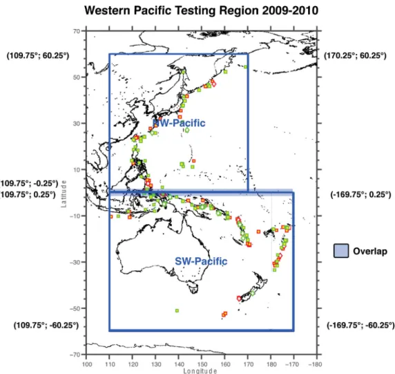
In this article, we analyse the experiments in the western Pa-cific (see Fig. 1). Because this a large region with a high rate of large earthquakes and because its seismicity as a whole is best described by the Global Centroid Moment Tensor (GCMT,

www.globalcmt.org; Dziewonski et al. 1981; Ekstr¨om et al. 2005) catalogue, the western Pacific region can be thought of as a pro-totype for future global earthquake predictability experiments. The western Pacific experiment is also useful for thinking about global earthquake forecast design. For example, it is generally thought that by considering only large earthquakes one can lower the fraction of triggered events (‘aftershocks’). This in turn can reduce the im-portance of declustering, which is sometimes applied to generate a catalogue that is well modelled by a Poisson process (see Sec-tion 4.2). Most CSEP models currently produce gridded forecasts that specify Poisson expectations in each bin, although regional earthquake observations are typically not Poisson (Werner & Sor-nette 2008; Lombardi & Marzocchi 2010).

The testing region and many of the metrics we applied were de-signed by CSEP researchers and this article is meant as a summary and discussion of the first results available. In addition to the stan-dard CSEP consistency tests, we also applied the recently proposed

T - and W - comparison tests (Rhoades et al. 2011).

Along with the location and magnitude details publicly reported in the GCMT catalogue, we obtained estimates of the location and seismic moment uncertainties, which we used to estimate the un-certainties of the evaluation metrics. While one expects the value of each metric to fluctuate with slightly different earthquake source parameter values, we are primarily interested in the stability of the

(2)

Figure 1. A sketch of the two test regions and their overlap, together with the target earthquakes for 2009 (red) and 2010 (green).

decision to which each evaluation is reduced: is the measured value statistically significant? The uncertainties estimation is new to the forecast testing and currently not part of the official CSEP methods. In the following section, we present the testing region. In Sec-tion 3, we describe the three models considered in this experiment. We then provide details related to the data source (Section 4) and the evaluation methods and related uncertainty estimation (Section 5). In Section 6, we present the primary results of the experiment and we discuss the experiment in general in Section 7. We conclude with a summary in Section 8.

2 T E S T I N G R E G I O N

Because the CSEP western Pacific experiment was based on the work of Kagan & Jackson (1994) and Jackson & Kagan (1999), the testing region in this experiment is the same used in that work and others (e.g. Kagan & Jackson 2000, 2010). In particular, the western Pacific is broken into two regions—the northwest Pacific and the southwest Pacific—with slight overlap; this region is shown in Fig. 1. The northwest Pacific covers the longitude range between 109.75 and 170.25 and the latitude range between−0.25 and 60.25 and the southwest Pacific covers longitudes 109.75 to−169.75 and latitudes−60.25 to 0.25. Both sub-regions are gridded into cells of 0.5◦by 0.5◦and only earthquakes with a magnitude Mw≥ 5.8 and

depth d≤ 70 km are considered. Unlike other CSEP experiments, all earthquakes above the minimum target magnitude are treated

the same; there is no binning of magnitudes for the forecasts or the observations.

The western Pacific testing region includes much of the ‘Ring of Fire’ and spans a variety of tectonic regimes, including the subduc-tion that dominates Japan and the strike-slip faults of New Zealand. While it contains the CSEP testing regions being investigated in Japan and New Zealand, we note that the grid spacing in this study is much larger (0.1◦ by 0.1◦ is used in Japan and New Zealand), as is the minimum target magnitude (as small as 3.95 in the other regions). Regarding the high seismicity rate in the western Pacific, according to the GCMT catalogue 95 earthquakes above Mw≥ 5.8

and with depth d≤ 70 km occurred in this region in 2009, that is 54 per cent of all such earthquakes worldwide. In 2010, 139 such earthquakes were reported in the western Pacific, accounting for 63.2 per cent of these earthquakes worldwide. (We note that the region covers only about 13 per cent of Earth’s surface area.) These numbers imply that the western Pacific region is well-suited for stud-ies of large earthquakes, because it typically takes only one year to collect samples of more than 100 events with which to evaluate prospective forecasts.

3 M O D E L S

Three models participated in this experiment: DBM, the double branching model (Marzocchi & Lombardi 2008); KJSS, the Kagan and Jackson smoothed seismicity model (Kagan & Jackson 2000,

(3)

A prospective earthquake forecast experiment in the western Pacific 1581

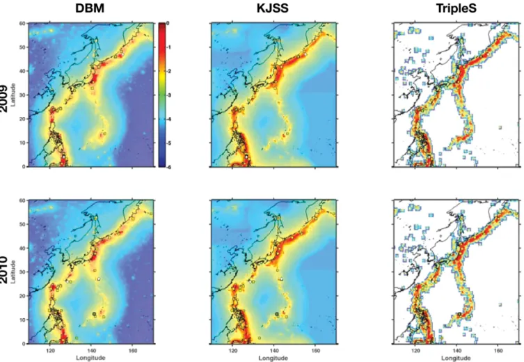
Figure 2. The maps show the base-10 logarithm of the forecast rates for each of the three models in the NW Pacific test region for 2009 (top row) and 2010 (bottom row). The dots are the locations of the target earthquakes. Regions in white indicate zero forecast rate.

2010) and TripleS, the simple smoothed seismicity model (Zechar & Jordan 2010). All three are statistical models that use past seismicity as their input and they thus represent only a small portion of the possible model space. Certainly, future experiments should include a broader variety of models that represent various hypotheses of earthquake occurrence.

The Epidemic Type Aftershock Sequence (ETAS) model (Ogata 1988, 1989) has been used many times to model individual aftershock sequences and regional seismicity, particularly em-phasizing short-term variations in seismicity rate (Ogata 1999, 2011). ETAS represents seismicity with a stochastic point process and incorporates the best-studied empirical seismicity relations: the Gutenberg–Richter distribution of magnitudes (Gutenberg & Richter 1954) and the Omori–Utsu relation which describes the tem-poral decay of aftershock productivity (Omori 1894; Utsu 1961). Marzocchi & Lombardi (2008) found that a two-step application of ETAS—one for short-term behaviour and one for long-term behaviour—provided a superior fit to global seismicity. Because ETAS is a branching model, Marzocchi & Lombardi called their model the Double Branching Model.

Kagan & Jackson (2000) described a short-term and a term seismicity model; in this study, we considered only the long-term model, which uses smoothed seismicity with an anisotropic smoothing kernel to estimate seismicity rates and does not in-clude any time dependence. The anisotropic smoothing kernel is designed to better account for the effects of the finite faulting of large earthquakes.

The TripleS is the simplest model in this experiment. The TripleS model was designed to be a plausible reference model for com-parison with more sophisticated models (Zechar & Jordan 2010). TripleS uses an isotropic Gaussian smoothing kernel with only one parameter to smooth past seismicity and construct a predictive den-sity. Because it is not clear what is the ‘right’ way to decluster a seismicity catalogue (see e.g. van Stiphout et al. 2011, 2012), the TripleS implementation in this experiment was based on a catalogue that is not declustered. The other models account for triggered earth-quakes, but they do this internally (i.e. the catalogue used to train the models need not be declustered before processing).

A visual comparison of forecasts generated by the three models reveals some common features (see Figs 2 and 3) and some features that are unique to each model. The DBM forecasts have remarkably small-scale variations outside the primary zones of seismicity; this is probably due to the way short-term variations are treated. On the other hand, the KJSS forecasts have pronounced peaks in some cells in the southwest Pacific (see Table 1). Unique to the TripleS model is the minimum forecast rate, which in contrast to the other models is set to zero. The zero rate is caused by an optimization in the model code (see Zechar & Jordan 2010, eq. 5). We note that this is a potentially grave problem for the model, because this implies that it is impossible for a target earthquake to occur in one of these cells. If an earthquake would occur, it would immediately invalidate the TripleS forecast.

All forecasts were automatically generated by codes submitted to the Southern California Earthquake Center CSEP testing centre by

(4)

Figure 3. Same as Fig. 2 for the SW Pacific region.

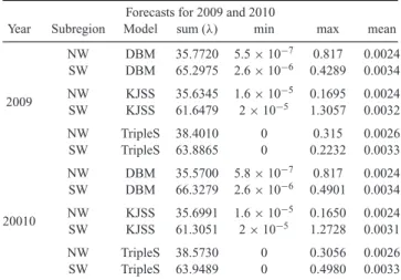
Table 1. For the 2009 and the 2010 forecasts, the overall forecast rate, the minimum/maximum rate in all cells and the average rate.

Forecasts for 2009 and 2010

Year Subregion Model sum (λ) min max mean

NW DBM 35.7720 5.5× 10−7 0.817 0.0024 SW DBM 65.2975 2.6× 10−6 0.4289 0.0034 NW KJSS 35.6345 1.6× 10−5 0.1695 0.0024 2009 SW KJSS 61.6479 2× 10−5 1.3057 0.0032 NW TripleS 38.4010 0 0.315 0.0026 SW TripleS 63.8865 0 0.2232 0.0033 NW DBM 35.5700 5.8× 10−7 0.817 0.0024 SW DBM 66.3279 2.6× 10−6 0.4901 0.0034 NW KJSS 35.6991 1.6× 10−5 0.1650 0.0024 20010 SW KJSS 61.3051 2× 10−5 1.2728 0.0031 NW TripleS 38.5730 0 0.3056 0.0026 SW TripleS 63.9489 0 0.4980 0.0033

the experiment participants. The forecasts generated for 2009 could use any GCMT data available before 2009 and the 2010 forecasts could also include the observations from 2009.

4 D AT A S O U R C E 4.1 Data preparation

The GCMT catalogue (Dziewonski et al. 1981; Ekstr¨om et al. 2005) was used for both model building and evaluation. We com-piled the evaluation catalogue by concatenating the monthly files available from the CMT homepage (http://www.ldeo.columbia.edu/

gcmt/projects/CMT/catalog/NEW_MONTHLY/). The exact cata-logues used to evaluate the forecasts are available in the Supporting Information section. We used the the centroid location for the earth-quake location and the moment magnitude Mwderived from total

moment M0 for the magnitude. We calculated Mw from M0using

the formula suggested by the GCMT catalogue curators

Mw= (2/3)(log M0− 16.1) (1)

To be consistent with the moment magnitudes reported by the GCMT web interface, we rounded the resulting magnitudes to the nearest 0.1.

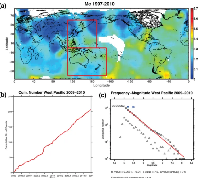
Kagan (2003) estimated that the GCMT catalogue is complete for earthquakes above Mw= 5.3 for shallow earthquakes (0–70 km

depth) since 1997 (see his Table 1). For 2009 and 2010, we esti-mated completeness using the maximum curvature method (Wiemer & Wyss 2000) and the entire magnitude range (EMR) method (Woessner & Wiemer 2005) and estimate that the GCMT is com-plete above Mw= 5.4 for both years (see Fig. 4).This is far below

the target magnitude threshold of Mw= 5.8 and we are therefore

confident that the target earthquake catalogues are not missing any earthquakes. This also implies that we could test with a minimum target magnitude of Mw= 5.4, but the models thus far only make

forecasts for events above Mw= 5.8.

4.2 Mainshocks and aftershocks

Part of the motivation for considering large target earthquakes is the expectation that such an experiment should contain fewer trig-gered earthquakes than regional catalogues of smaller events. This is important because, to date, CSEP forecasts are almost always stated in terms of expected rates and characterized by a Poisson

(5)

Figure 4. (a) Magnitude of completeness map using EMR for shallow earthquakes (0–70 km) in the GCMT catalogue from 1997 to 2001. We used a grid spacing of 2.5◦with at least 25 but not more than 300 events at a maximum distance of 3000 km from each grid cell. Marked in red are the two testing regions. (b) The cumulative number of earthquakes in the western Pacific testing region through 2009 and 2010. (c) Frequency–magnitude distribution in the western Pacific testing region for 2009–2010.

distribution, implying that the the forecast bins are independent. A high percentage of aftershocks would violate this assumption.

It is possible to remove triggered earthquakes by so called declus-tering of an earthquake catalogue (e.g. Knopoff 1964; Gardner & Knopoff 1974). But because there is no known physical property that allows one to distinguish between mainshocks and aftershocks, declustering yields non-unique solutions and it can have a strong effect on any analysis that follows. Various methods have been pro-posed to decluster a catalogue, each of them with its advantages and disadvantages, but the ‘right’ method for any given application is unknown (van Stiphout et al. 2011, 2012).

In this experiment the target earthquake catalogue is not declus-tered. Experiment participants agreed to target a clustered catalogue at the beginning of the experiment and each model has its own way to deal with aftershocks in the catalogue (see Section 3).

5 M E T H O D S

CSEP testing centres currently use various tests to determine which models fit the observed data and which models forecast the dis-tribution of seismicity best (see e.g. Zechar et al. 2010a; Rhoades

et al. 2011). The tests can be grouped in two categories: consistency

and comparison. Most of the tests described in this article are im-plemented in CSEP testing centres and results can also be viewed online (http://www.cseptesting.org). For this study we used a custom implementation of the tests so we could estimate uncertainties.

5.1 Consistency tests

The principle behind each consistency test is the same. One cal-culates a goodness-of-fit statistic for the forecast and the observed data. One then estimates the distribution of this statistic assuming

(6)

that the forecast is the data-generating model (by simulating cata-logues that are consistent with the forecast). One then compares the calculated statistic with the estimated distribution; if the calculated statistic falls in lower tail of the estimated distribution, this implies that the observation is inconsistent with the forecast or that the fore-cast should be ‘rejected’. For the CSEP consistency tests used here, the likelihood is the fundamental metric, but this approach would be similar for different statistical measurements.

We applied three straightforward consistency tests: the

N (number)-test, the S(space)-test and the L(likelihood)-test (Zechar et al. 2010a). The N -test compares the total number of earthquakes

forecast with the the number observed, checking if the overall fore-cast rate is too high or too low. When applied to Poisson forefore-casts, the N -test involves exact analytical solutions and therefore requires no simulations. The N -test result is summarized by two quantile scores,δ1 and δ2. If either of these scores are below the critical

threshold value, the forecast is rejected as overpredicting or under-predicting, respectively. For the tests in this study, we used a critical value of 0.05, corresponding to 95 per cent confidence in each re-sult. Because the N -test is a two-sided test, the effective critical value for it is 0.025.

The S-test evaluates the consistency of the forecast spatial dis-tribution with the observed epicentres: this is done by summing over all magnitude bins within each spatial cell and normalizing the resulting rates such that the overall forecast rate matches the observed number of earthquakes. Then the spatial Poisson joint log-likelihood of the binned observation given the forecast is com-puted. The resulting quantile scoreζ is the fraction of simulated spatial joint log-likelihoods that are smaller than the observed one. It has been noted that very high values ofζ should not be used to reject a forecast (Zechar et al. 2010a) and therefore the S-test is one-sided.

The M-test is similar to the S-test but uses instead the magnitude bins: it is meant for checking the consistency of a forecast with the observed magnitude distribution. Because we only have one magnitude bin per spatial cell, the M-test is not applicable to this study.

The L-test can be thought of as a convolution of the three other tests L = N × S × M. For the L-test, the metric of interest is the likelihood for each magnitude bin in each spatial cell. In other words, the L-test evaluates the joint distribution implied by the forecast and doesn’t involve any normalization or dimensional re-duction. It is also possible to combine the S-test and M-test and normalize the rates of the model to the total number of earth-quakes in the observation: the resulting test is called the conditional

L-test or LN-test (Rhoades et al. 2011; Werner et al. 2010). Rhoades

et al. asserted that the LN-test together with N -test is often more

informative than the L-test alone, but for the western Pacific testing region the LN-test is exactly equivalent to the S-test because each

forecast has only one magnitude bin. Like the S-test, the L-test is one-sided.

The likelihood R(ratio)-test was originally proposed as a com-parison test for the RELM experiment (Schorlemmer et al. 2007, 2010b). The R-test is in principle similar to the L-test, but fore-casts are considered in pairs where one is taken as the reference and assumed to have come from the data-generating model and the other is taken as an alternative. And rather than considering the joint log-likelihood of one model, the ratio of the two likelihoods (L(ref .model)− L(alt.model)) is used.

As others (Rhoades et al. 2011; Marzocchi et al. 2012) have noted, the R-test results are difficult to interpret. The R-test does not identify the model with the higher likelihood, it is another test

of consistency: a small quantile score seems to indicate that the reference model is inconsistent with observed data, but it does not imply that the alternative model is superior. We note that Kass & Raftery (1995, p. 789, their Point 4) described exactly this type of difficulty in a more general context. Because of this confusion, we did not apply the R-test in this study.

In our implementation of these tests, we simulated 5000 cata-logues for each test.

5.2 Comparison tests

The goal of the comparison tests is to compare the different models and decide which provides the best fit to the observations. These tests complement the consistency tests because they answer the question ‘Which of two models is better?’, but not ‘How good is each model?’ In this study, we applied the T -test and the W -test as described by Rhoades et al. (2011). Both tests are based on the same measurement: the information gain for observed target earthquakes. For each pair of forecasts, one finds the spatial cell in which the first target earthquake occurred; one then computes the logarithm of the ratio of the forecast rates in this cell; this ratio is also well known as the probability gain. One then repeats this process for all target earthquakes and computes the average information gain per earthquake. This quantity should then be corrected for overall rate differences: otherwise, a forecast with very high rates everywhere would always seem superior.

These quantities have connections to other work: for exam-ple, the information gain in this context is closely related to the Kullback–Leibler distance and the information theory concept of relative entropy (Harte & Vere-Jones 2005).

The T -test is an application of Student’s paired t-test (Student 1908) to the rate-corrected information gains and it asks the ques-tion: is the rate-corrected average information gain per earthquake significantly different from zero? In other words, is one of the fore-casts significantly better than the other?

The T -test assumes that the individual rate-corrected information gains are normally distributed. Because this assumption may be violated, we also consider the W -test, which is an application of the Wilcoxon signed-rank test (Wilcoxon 1945) to the same quantities. The W -test only assumes a symmetric distribution of the measures, but it is also less powerful than the T -test if the assumptions behind the T -test are not violated (Rhoades et al. 2011).

As a benchmark and in the spirit of Werner et al. (2010), we also compared each forecast with a spatially uniform forecast and the ‘perfect’ forecast. The perfect forecast has a rate equal to the number of observed target earthquakes in each cell. These comparisons give the reader an idea of how much each forecast could be improved.

5.3 Uncertainty estimation

An estimate of each metric’s uncertainty is useful to judge the reli-ability and robustness of the forecast testing. To make this estimate, we considered the uncertainty associated with each earthquake’s location and size.

In general, the uncertainty of an earthquake location and size is difficult to quantify (Husen & Hardebeck 2010); for the GCMT catalogue, the centroid location uncertainties have been previously estimated to be isotropic and Gaussian with one standard deviation being 30 km (Smith & Ekstr¨om 1997). The uncertainties of the magnitudes are expressed in terms of the standard deviation of the total moment, which is given byσM0= 0.2× M0(M. Nettles 2011,

(7)

We used these location and total moment uncertainties to generate 1000 perturbed catalogues with modified locations and magnitudes. The construction of a perturbed catalogue involves the following steps: The location of each earthquake in the whole unfiltered cata-logue is modified by adding an offset to the longitude and latitude. The offset is drawn from a 2-D Gaussian distribution with the re-ported location as the mean and the standard deviation equal to the centroid location uncertainty. A similar technique is applied for the total moment of the earthquakes (although using a 1-D Gaussian distribution). The moment magnitude Mw is then calculated from

the total moment using eq. (1). This constructed perturbed raw cat-alogue is then filtered so that only target events falling within the test regions remain.

We calculated the quantile score of each test for each perturbed catalogue using the same simulated catalogues that were used when comparing the forecast with the observed catalogue. From the re-sulting distribution of ‘perturbed’ quantile scores, basic statistical measurements like a mean quantile score and a standard deviation of the score can be calculated. In this study, we report the median and the 16th and 84th percentile of the consistency scores. We re-port these values rather than the mean and a standard deviation because the domain of possible consistency quantiles scores is lim-ited (by definition, they are restricted to values between 0 and 1) and therefore the perturbed scores might not be symmetric. For the comparison tests, we report the mean value with sample stan-dard deviation, as the information gain is not limited and should be approximately normally distributed.

The perturbation procedure affects not only the observed target earthquakes within the testing region and above the minimum target magnitude, but it also allows earthquakes to jump into (or fall out of) the test region criteria and thus change the total number of earthquakes in the test.

We note that all of the modellers targeted the observed catalogue and therefore they are slightly disadvantaged when we compare their forecasts with perturbed catalogues and because of this, we do not consider the uncertainty estimation to be an ‘official’ part of CSEP experiment. Nevertheless, the disadvantage should be rela-tively minor and affect all forecasts equally.

6 R E S U L T S

In this section, we present the primary results for all three forecasts for both testing regions (southwest Pacific and northwest Pacific) and both years (2009 and 2010), and we also report the results of the experiment as a whole by combining both years and testing regions, which we think gives a good summary of the models’ performances. We primarily emphasize the comparison test results and selected consistency test results; comprehensive test results are available in the Supporting Information section and on the CSEP webpage (http://cseptesting.org/results).

6.1 Consistency of the forecasts

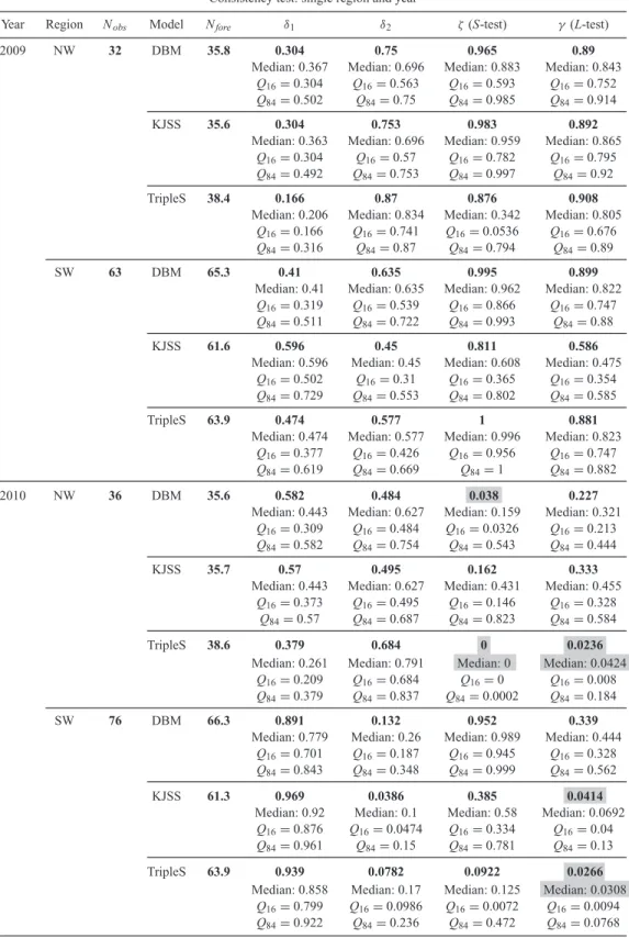
We report the results of the consistency tests for each year and each testing region in Table 2. In 2009, all models slightly overestimated the total number of earthquakes in both regions, except KJSS in SW Pacific. Nevertheless, the overall forecast rates are consistent with the observed rates (i.e. no value ofδ1orδ2is below the critical

value). In 2009 the S-test scores (ζ in Table 2) indicate reason-able agreement between the spatial component of each forecast and the observations: no forecast fails the S-test. Likewise, the 2009

L-test results (γ in Table 2) indicate the overall consistency of the

models with the observations: all forecasts also pass this test. For the observations of 2010, the results are slightly different. Many more earthquakes happened in both regions in 2010, espe-cially in the SW Pacific and as a result all models underestimated the total number of earthquakes except the TripleS model in the NW Pacific region. The N -test scores (δ1andδ2in Table 2) reflect these

underestimations, but in both regions all forecasts pass the N -test for 2010.

On the other hand, the results of the S-test are less clear for 2010. In the NW Pacific only KJSS passes the S-test: both DBM and TripleS fail due to earthquakes happening in places where these models produce very low forecast rates. For TripleS, one earthquake occurred in a bin with a forecast rate of 10−10, but no earthquake occurred in any cell with zero rate. In the SW Pacific, all forecasts pass the S-test, although TripleS is only a borderline pass. Unsurprisingly, not all forecasts pass the L-test (γ ). In the NW Pacific TripleS fails the L-test, a result which is also explained by exceedingly poor spatial performance. Also in the NW Pacific, DBM passes the L-test although it did not pass the S-test: this is understandable because its spatial performance is not as bad as that of TripleS. In the SW Pacific region KJSS and TripleS both fail the

L-test and both failures are a combination of relatively poor spatial

performance and relatively large underestimation.

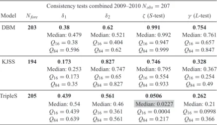
By treating both years and both regions jointly, we also calculated a combined score for each model (see Table 3). Due to the higher number of observations in this combined score the influence of a single earthquake or a few earthquakes in cells with very low forecast rates is less strong and accordingly, in this view all models are consistent with the observation although again TripleS is only a borderline pass on the S-test.

6.2 Comparison of the forecasts

Differences in consistency test quantile scores do not allow a direct ranking of the models. The likelihood of the forecasts per earthquake (see Table 4) gives some ranking but does not allow a statistical hypothesis test. On the other hand, the comparison tests provide us with a clear ranking of the forecasts. We applied each comparison test to each pair of forecasts and the results are summarized in Tables 5 and 6. For each test, we report the average information gain and its confidence interval for the observed catalogue, together with a p value for the T -test and for the W -test. We also report the mean value and an associated standard deviation for the perturbed catalogues (see the Supporting Information section). In theory the tests are perfectly symmetric, but because random numbers are used to construct the perturbed catalogues, some negligible differences occur.

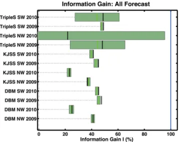
For 2009 the T -test and W -test suggest the following ranking (see Table 6): TripleS, DBM and KJSS. This ranking can also be derived by examining the average information gain against a uniform rate forecast (see Fig. 5). The confidence interval of the T -test and the

p values tell us that the differences in average information gain are

significant for the NW Pacific but not for SW Pacific. There the difference between TripleS and DBM is not significant according to the T -test and the W -test. For the T -test in SW Pacific, the difference between DBM and KJSS is not statistically significant.

In 2010, the ranking is slightly different and not as clear: in the NW Pacific, the T -test suggests a ranking of DBM, KJSS, TripleS (see Table 6), while the W -test suggests TripleS, DBM, KJSS. It is worth noting that the T -test suggests that the

(8)

Table 2. Results from the consistency tests of both subregions and both time periods. Nobsis the number of observed

earthquakes, Nforethe expectation value of each forecast,δ1andδ2are the two scores of the N-test,ζ is the score of

the S-test andγ is the score of the L-test. For each cell, the first row is the score of the forecast measured against the observed catalogue, and the second, third and fourth row are the scores of the forecast against the perturbed catalogues, described by the median score, the 16th percentile score and the 84th percentile score. Shaded cells indicate scores lower than the threshold (i.e. test failures).

Consistency test: single region and year

Year Region Nobs Model Nfore δ1 δ2 ζ (S-test) γ (L-test)

2009 NW 32 DBM 35.8 0.304 0.75 0.965 0.89

Median: 0.367 Median: 0.696 Median: 0.883 Median: 0.843 Q16= 0.304 Q16= 0.563 Q16= 0.593 Q16= 0.752

Q84= 0.502 Q84= 0.75 Q84= 0.985 Q84= 0.914

KJSS 35.6 0.304 0.753 0.983 0.892

Q84= 0.492 Q84= 0.753 Q84= 0.997 Q84= 0.92

TripleS 38.4 0.166 0.87 0.876 0.908

Q84= 0.316 Q84= 0.87 Q84= 0.794 Q84= 0.89

SW 63 DBM 65.3 0.41 0.635 0.995 0.899

Q84= 0.511 Q84= 0.722 Q84= 0.993 Q84= 0.88

KJSS 61.6 0.596 0.45 0.811 0.586

Q84= 0.729 Q84= 0.553 Q84= 0.802 Q84= 0.585

TripleS 63.9 0.474 0.577 1 0.881

Q84= 0.619 Q84= 0.669 Q84= 1 Q84= 0.882

2010 NW 36 DBM 35.6 0.582 0.484 0.038 0.227

Q84= 0.582 Q84= 0.754 Q84= 0.543 Q84= 0.444

KJSS 35.7 0.57 0.495 0.162 0.333

Q84= 0.57 Q84= 0.687 Q84= 0.823 Q84= 0.584

TripleS 38.6 0.379 0.684 0 0.0236

Median: 0.261 Median: 0.791 Median: 0 Median: 0.0424 Q16= 0.209 Q16= 0.684 Q16= 0 Q16= 0.008

Q84= 0.379 Q84= 0.837 Q84= 0.0002 Q84= 0.184

SW 76 DBM 66.3 0.891 0.132 0.952 0.339

Q84= 0.843 Q84= 0.348 Q84= 0.999 Q84= 0.562

KJSS 61.3 0.969 0.0386 0.385 0.0414

Q84= 0.961 Q84= 0.15 Q84= 0.781 Q84= 0.13

TripleS 63.9 0.939 0.0782 0.0922 0.0266

(9)

A prospective earthquake forecast experiment in the western Pacific 1587 Table 3. Columns and cell contents have the same meaning as in Table 2.

Consistency tests combined 2009–2010 Nobs= 207

Model Nfore δ1 δ2 ζ (S-test) γ (L-test)

DBM 203 0.38 0.62 0.991 0.754

Q84= 0.596 Q84= 0.62 Q84= 0.999 Q84= 0.847

KJSS 194 0.173 0.827 0.746 0.328

Q84= 0.35 Q84= 0.827 Q84= 0.933 Q84= 0.49

TripleS 205 0.439 0.561 0.0506 0.262

Q84= 0.639 Q84= 0.561 Q84= 0.217 Q84= 0.366

Table 4. Log-likelihood per earthquake and spatial log-likelihood per earth-quake. Shaded cells indicate scores lower than the threshold (i.e. test fail-ures).

Model Log-likelihood Spatial log-likelihood per earthquake per earthquake

NW Pacific 2009 NW DBM 2009 −4.6980 −4.6915 NW KJSS 2009 −4.9750 −4.9690 NW TripleS 2009 −4.2309 −4.2132 SW Pacific 2009 SW DBM 2009 −4.0210 −4.0203 SW KJSS 2009 −4.1578 −4.1576 SW TripleS 2009 −3.9328 −3.9327 NW Pacific 2010 NW DBM 2010 −5.5372 −5.5371 NW KJSS 2010 −5.6521 −5.6520 NW TripleS 2010 −5.7399 −5.7375 SW Pacific 2010 SW DBM 2010 −4.0527 −4.0439 SW KJSS 2010 −4.2892 −4.2677 SW TripleS 2010 −3.8548 −3.8407

differences are not statistically significant, which is evident from the large TripleS T -test standard deviations. These large standard deviations and the fact that the T -test and W -test suggest such dif-ferent rankings can be explained by an apparent violation of the

T -test assumptions (see Section 7.1). In the SW Pacific, the T -test

and W -test suggest the same almost always statistically significant ranking as in 2009 (see Table 6): TripleS, DBM, KJSS (see also Fig. 5), only the W -test between TripleS and DBM suggests a lack of significance.

The combination of both testing regions and both years into a single test result (see Table 5 and Fig. 6) leads to the same ranking as the majority of tests suggests: TripleS, DBM and KJSS. Apart from the T -test between DBM and TripleS all tests suggest statistically significant differences between the forecasts.

6.3 Uncertainty of the results

Following our method to estimate the uncertainty of consistency metrics, we report a median and the 16th and 84th percentile of

the score distribution resulting from perturbed target earthquake catalogues. For the comparison tests, we report the mean and the sample standard deviation instead. It is important to notice that the score calculated with the observed catalogue is normally not identical to the median or mean of the test scores from perturbed catalogues. For consistency tests the median is normally larger than the original score when the original score is below 0.5 and smaller if the original score is above 0.5 (see Section 7.2). This effect is not always observable in the combined scores (see Fig. 7). For the comparison tests, the differences between the mean values for each forecast are generally smaller than the differences between the observed values.

The most important difference between the observed scores and the perturbed scores is that for some consistency tests, the outcome would be different if the median of the perturbed scores were used. The distribution of the perturbed scores varies strongly between the different tests, models and regions. Generally, the S-test tends to have broadest distribution: in some cases the perturbed S-test scores are distributed almost uniformly over the whole range (see Fig. 7). In such cases the median and the 68 per cent interval are not a very useful representation of perturbed scores. The influence of the perturbation on the comparison tests is much smaller: except for the tests involving the TripleS forecast for NW Pacific in 2010, the observed information gain and mean perturbed information gain are in good agreement.

7 D I S C U S S I O N

In our analysis of the two contiguous 1-yr experiments, we find different results. In 2009, all forecasts were consistent with the observations and we obtained an unambiguous (albeit not always statistically significant) ranking of the models from the comparison tests. On the other hand, in 2010 several forecasts failed consistency tests, including the model that the comparison tests identified as having the highest information gain.

One conspicuous difference between the two years of data is the total number of earthquakes. While the observation of 36 earth-quakes in 2010 NW Pacific is not anomalous compared to previous 1-yr periods, the 76 earthquakes in SW Pacific for 2010 make this one of the most productive 1-yr periods on record. This explains the relatively poor performance of the models in the N -test for SW Pacific 2010, but it alone does not explain the failure in the S-test for both regions in 2010. As we mentioned, a ‘surprise’ earthquake in a location with a historically low seismicity rate could explain

(10)

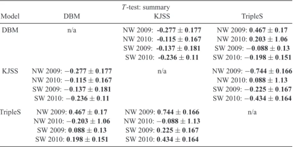
Table 5. Results of T -test for each pair of models for each year and each region. For each cell, the row header indicates the reference model and the column header indicates the alternative model. In each cell we report the rate-corrected average information gain per earthquake and its confidence interval for the observed catalogue.

T -test: summary Model DBM KJSS TripleS DBM n/a NW 2009: -0.277± 0.177 NW 2009: 0.467 ± 0.17 NW 2010: -0.115± 0.167 NW 2010: 0.203 ± 1.06 SW 2009: -0.137± 0.181 SW 2009:−0.088 ± 0.13 SW 2010: -0.236± 0.11 SW 2010:−0.198 ± 0.151 KJSS NW 2009:−0.277 ± 0.177 n/a NW 2009:−0.744 ± 0.166 NW 2010:−0.115 ± 0.167 NW 2010: 0.088 ± 1.13 SW 2009:−0.137 ± 0.181 SW 2009:−0.225 ± 0.167 SW 2010:−0.236 ± 0.11 SW 2010:−0.434 ± 0.164 TripleS NW 2009: 0.467 ± 0.17 NW 2009: 0.744 ± 0.166 n/a NW 2010:−0.203 ± 1.06 NW 2010:−0.088 ± 1.13 SW 2009: 0.088 ± 0.13 SW 2009: 0.225 ± 0.167 SW 2010: 0.198 ± 0.151 SW 2010: 0.434 ± 0.164

Table 6. Results of comparison tests for each pair of models for the combined region and both years. For each cell, the row header indicates the reference model and the column header indicates the alternative model. In each cell we report the rate-corrected average information gain per earthquake and its confidence interval for the observed catalogue (first line), the p-value of the T -test (second line), the p-value of the W -test (third line), the mean rate-corrected average information gain with its standard deviation (fourth line) and the mean confidence interval with its standard deviation (fifth line). Note that the values on the fourth and fifth lines correspond to the perturbed catalogues.

Comparison tests combined 2009–2010

Model DBM KJSS TripleS

DBM n/a 0.191 ± 0.0781 −0.124 ± 0.193

PT= 3.88e − 05 PT= 0.146

PW = 2.54e − 07 PW= 1.19e − 05

0.174± 0.0317 0.557± 1.41 conf. Int. 0.0834± 0.00427 conf. Int. 1.16± 2.14

KJSS −0.191 ± 0.0781 n/a −0.314 ± 0.208

PT= 3.88e − 05 PT= 0.00669

PW= 2.54e − 07 PW= 3.17e − 12

−0.175 ± 0.0321 0.446± 1.48

conf. Int. 0.0833± 0.00425 conf. Int. 1.27± 2.24

TripleS 0.124 ± 0.193 0.314 ± 0.208 n/a

PT= 0.146 PT= 0.00669

PW= 1.19e − 05 PW = 3.17e − 12

−0.585 ± 1.45 −0.463 ± 1.54

conf. Int. 1.2± 2.19 conf. Int. 1.28± 2.27

S-test failures. To determine how ‘normal’ such failures are, more

test data are required.

7.1 T-test and W-test

The discrepancies between the consistency tests and the comparison tests and the discrepancies between the T -test and the W -test are worth further consideration. In 2010 in the SW Pacific, TripleS is ranked highest by the comparison tests (see Fig. 5) despite being re-jected by consistency tests. Additionally, in the NW Pacific in 2010, the T -test and W -test suggest different rankings and the confidence interval for the TripleS T -test (see Table 6) is much broader than for all other tests. To understand these results, we consider the limits of the tests and how each treats forecasts with very low rates.

Both the T -test and the W -test use the same measures— sample information gain—but they process them differently. In the

T -test, the amplitude of the sample information gains is emphasized,

whereas the W -test emphasizes the sign of the sample information gains. Consider the situation where the sample information gains are all slightly positive except one value which is extremely neg-ative. It is likely that the T -test and W -test would yield different conclusions: the T -test would be dominated by the extreme value, while the W -test would not. Moreover, this situation would violate the normality assumption of the T -test. Indeed, in 2010 in NW Pa-cific, the situation is similar and this is also the likely cause of the large confidence interval in the TripleS T -test.

Unlike the comparison tests, the consistency tests punish quite severely a forecast with an extremely low forecast rate where an

(11)

Figure 5. Average information gain of the forecast expressed in terms of in percentage of ‘maximum possible’ information gain given by the ‘perfect’ forecasts. The solid black line shows information gain with respect to the observed catalogue and the solid green line and the green area show the mean and the values within one standard deviation, respectively, of the information gain with respect to the perturbed catalogues.

earthquake occurred (see e.g. section 7 of Holliday et al. 2005). The comparison tests and particularly the W -test, tend to be less sensitive to individual earthquakes. This is in the end not a big problem, because it could mean that the ‘winning’ model is good but has some flaws such as not being smooth enough.

The W -test has one additional caveat: when two models produce the exact same forecast rate for a bin containing one or more tar-get earthquakes, this bin will be ignored. In the situation that two forecasts have many common rates where earthquakes occurred, a small difference might spuriously appear to be statistically signifi-cant. Nevertheless this is rarely a problem in practice, as two models seldom produce the exact same forecast value where an earthquake occurred.

In the spirit of Sawilowsky & Blair (1992), we also used simu-lations to estimate the power of the T -test and W -test for the three models considered in this study. The details of these simulations are included in the Supporting Information section and we men-tion only that, for the number of target earthquakes used in these experiments, both tests have high power.

The question of which comparison test should be preferred is a difficult one. The T -test emphasizes single large differences between forecasts. The W -test de-emphasizes large differences and accounts more for the overall performance in all the earthquakes. Both tests do the same thing but do it slightly differently and we suggest that both tests should be applied, along with the consistency tests, as each test analyses different aspects of the models. At the same time, we emphasize that one should carefully study the results of each test and each experiment when interpreting the results.

7.2 Perturbed scores versus observed score

Ideally, the difference between the median or mean score from the perturbed catalogues and the score from the observed catalogue would be as small as possible. More generally, one would prefer that the catalogue uncertainties not affect the decision whether or not to reject a forecast. However, this is not the case in 2010: in both testing regions the decision would change if the median of the score were used instead of the score from the observed catalogue. Nevertheless, for this study, modellers were specifically asked to forecast the observed (noisy) catalogue, not a suite of perturbed catalogues taking uncertainty into account. Therefore, we consider the observed score to be authoritative. On the other hand, the scores from the perturbed catalogues are useful for exploring result stability and future experiments may target perturbed catalogues.

Moreover, the perturbed catalogues allow a good practical as-sessment of model stability and also a hint about how exceptional a certain period is. For each test the median of the scores depends on the locations of earthquakes within the forecast. If many earth-quakes are located either at a part of the forecast where the differ-ences between neighbouring grid cells are large or at the boundary

Figure 6. Combined results of the T -test and W -test for all forecasts. (a) Information gain of the models relative to a uniform rate forecast and a ‘perfect’ forecast (solid blue line). For each model the solid black line gives the information gain according to the observed catalogue, and the green line together with the green area indicate the mean and the values within one standard deviation, respectively, of the information gains according to the perturbed catalogues. Due to the good agreement between perturbed and observed information gain the difference between the two is barely visible. (b) p-values of the T -test (lower right corner) and the W -test (upper left corner). Fields with a significant difference in information gain are marked green while insignificant differences are marked red.

(12)

Figure 7. Results of the L-test, S-test and N -test, the green line marks the score according to the observed catalogue, solid blue line gives the median and shaded area the 68 per cent interval of the scores according to the perturbed catalogues. The dotted blue and green line gives the distribution of the scores from the perturbed catalogues. The red areas mark the threshold values for the scores. (a) shows the results of the combined scores for DBM and (b) shows the results for KJSS in northwest Pacific 2010.

of the testing region, the differences between median of the per-turbed scores and observed score can be quite large. Because the models considered here produce forecasts that are not very smooth, the location perturbations tend to balance borderline misses and hits. Forecasts with a low consistency tends to perform better on the perturbed catalogues while forecasts with a high consistency per-form worse, which explains why the median of the scores is mostly shifted towards 0.5. Under this logic, the perturbed scores hint that 2010 is indeed exceptional and the models just missed the correct locations and total numbers.

Because of the Gutenberg–Richter distribution of magnitudes one might expect that perturbed catalogues have on average more earthquakes than the original catalogue. Nevertheless, this is not the case for the data in this study. One explanation is that while there are more earthquakes below the magnitude threshold, the symmet-ric uncertainties applied on the total moment lead to asymmetsymmet-ric uncertainties in the moment magnitude, meaning that it is easier to drop out than jump in the testing region. These opposing effects— the Gutenberg–Richter distribution of magnitudes and asymmetric magnitude uncertainties—balance each other in this study.

To estimate metric uncertainty, we only considered epicentre and total moment and thus we may underestimate the total uncertainty. In particular, we did not account for uncertainties in the depth and time of each earthquake. For this experiment, any timing error is negligible, but depth uncertainty could have some appreciable influence, as depth uncertainties tend to be rather large, especially on the global scale (Bird & Liu 2007). Because there was no binning in depth for this experiment, accounting for depth uncertainty would only add or subtract earthquakes from the test region.

7.3 Is the sequence of large earthquakes in the western Pacific Poissonian?

One of the key assumptions of the forecast format used in this experiment and which is widely used within CSEP, is that the earth-quakes in the target catalogue are approximately Poisson distributed. To check this assumption, we compared the fit of a Poisson

distri-bution and a negative binomial distridistri-bution to the annual number of target earthquakes. For each distribution, we calculated the Akaike Information Criterion (AIC) (Akaike 1974) for the observed target earthquake catalogue. The AIC is 290.11 for the Poisson distribu-tion and 275.02 for the negative binomial distribudistribu-tion, indicating that the negative binomial provides a better fit to the data and that the Poisson assumption is not supported by the data. Many others have shown the same in different regions and for different magni-tude ranges (e.g. Werner & Sornette 2008; Kagan & Jackson 2010; Lombardi & Marzocchi 2010).

To explore the idea that catalogues of large earthquakes typically contain a smaller portion of triggered seismicity, we applied the declustering algorithms of Gardner & Knopoff (1974) and Reasen-berg (1985) to the observed target earthquake catalogue, and for simplicity we used parameters values that were applied by the orig-inal authors to analyse seismicity in California. Both of these algo-rithms seek to identify triggered earthquakes based on space–time clustering and they result in a catalogue being divided into two mutually exclusive sets: mainshocks and aftershocks.

Table 7 shows the percentage of aftershocks identified by the two different declustering procedures and, for comparison, the frac-tion of aftershocks identified by the Reasenberg algorithm for the RELM experiment in California (Schorlemmer et al. 2010b). The fraction of aftershocks in the western Pacific catalogue is quite different depending on which declustering algorithm is used: the Gardener–Knopoff procedure identifies more than twice the num-ber of aftershocks as the Reasennum-berg approach. The∼40 per cent of aftershocks found by Gardner–Knopoff seems to be unrealistically

Table 7. Percentage of aftershocks in each region’s catalogue ac-cording to the different declustering methods.

Region Declustering method Percentage of aftershocks NW-Pacific Gardner–Knopoff 41 per cent SW-Pacific Gardner–Knopoff 38 per cent

NW-Pacific Reasenberg 19 per cent

SW-Pacific Reasenberg 15 per cent

(13)

high given the large minimum magnitude; this might be because the parameter values used for analysing California seismicity are not appropriate for a region as large as the western Pacific. Nevertheless, we note that the fraction of aftershocks is comparable to that found for the RELM target earthquakes, which suggests that clustering is important even for large earthquakes and future global earthquake forecast experiments should account for such clustering, although it remains unclear how to do this best.

7.4 To combine or not to combine results

There are at least two ways of examining the results of the ongo-ing earthquake forecast experiment in the western Pacific testongo-ing region. One can split the experiment into sub-experiments of the individual years and individual testing regions (i.e. southwest Pa-cific and northwest PaPa-cific) or one can join everything into a single period and region. Both approaches have advantages and disadvan-tages: the joining approach allows for a general summary of model performance and the results are based on more data, but it may miss important details. And while the splitting approach can pro-vide granularity, the test results may not be stable from year to year or for different subregions, making model selection a difficult task. In this study, we applied both approaches to the experiment and for the most part, the results are consistent, indicating that TripleS performed better than DBM and DBM performed better than KJSS. We propose that a mixture of these splitting and joining methods is a good way to proceed in future experiments. The details of each subregion, each year and even each target earthquake are key for interpreting and understanding the test results, but being able to make broad summary statements about model performance is also important.

8 C O N C L U S I O N S

In the first two years of the CSEP earthquake forecast experiment in the western Pacific, it seems that the TripleS model, the simplest participating model, performed better than the DBM and KJSS models. Nevertheless, this result does not hold for all subdivisions of the data; for example, TripleS fails some consistency tests for individual years and sub-regions. If, in future experiments, it be-comes clear that TripleS outperforms DBM and KJSS, this might indicate that the minor complexities of DBM (branching processes for short- and long-term seismicity) and KJSS (anisotropic power-law smoothing kernel) are not worthwhile. Nevertheless, we remind the reader that these models represent only a very small portion of the potential model space and exploring other models and other model classes is very important.

Now that CSEP researchers have begun working with data, mod-els and tests that are appropriate for forecasts of large earthquakes over large regions, it seems natural to consider a global experiment. Based on our experience with the western Pacific experiment, we have several recommendations.

(1) As has been suggested previously and owing to its relative homogeneity, the GCMT catalogue is good for developing and test-ing models of large earthquakes. Moreover, the GCMT curators have made initial efforts to quantify location and magnitude uncer-tainties and these could be improved. Considering the unceruncer-tainties of GCMT locations and to reduce computational overhead, we rec-ommend a global grid spacing not smaller than the 0.5◦used here. Our analysis of magnitude completeness suggests that the mini-mum target magnitude for global experiments could be as low as

Mw= 5.5, as opposed to the Mw= 5.8 used in the western Pacific.

Depending on which models are used it may be still better to use a higher minimum target magnitude, because some models need a catalogue with a completeness up to two orders below the target magnitudes. In this case, a minimum target magnitude of Mw =

7 would be appropriate. There would be still enough target earth-quakes in the global catalogue to yield meaningful results at even such a large minimum magnitude.

(2) While only one magnitude bin was used for the western Pacific testing region, we suggest using magnitude bins for a global experiment. This would allow a comparison of forecast magnitude distributions and the observed one and also allow a filtering of results that only includes, Mw≥ 6 target earthquakes, Mw≥ 7 target

earthquakes, etc. More importantly it would also allow modellers to choose a higher minimum target magnitude, to prevent their model performance from being dominated by smaller earthquakes.

(3) We used a variety of statistical tests in this experiment and we suggest that at the current stage of research, every test that reveals some additional information about earthquake occurrence models should be used. Examples of metrics that should also be considered for a global experiment include the gambling score (Zhuang 2010) and the residuals (and corresponding graphical tests) described by Clements et al. (2011) and Clements (2011).

(4) We conclude that estimating test uncertainties caused by earthquake catalogue uncertainty is useful and should be done in fu-ture analyses of earthquake forecast experiments. Perhaps this will also demonstrate to catalogue curators that statistical seismology researchers are interested in having more careful estimates of earth-quake location and size errors. We also support the notion that in future experiments the assumption that earthquakes are well mod-elled by a Poisson process be abandoned. This will require some revisions to the CSEP infrastructure, in particular the test implemen-tations and some additional work by model developers to specify an alternative forecast distribution, but it will allow for more direct testing of the relevant scientific hypotheses.

A C K N O W L E D G M E N T S

We thank Bruce Shaw, Christine Smyth and Yan Kagan for insightful comments. We thank Ella Galvan-Speers for suggesting usage of the word ‘borderline’. We thank Arnaud Mignan for reading an early draft of the manuscript. We thank Masha Liukis for providing forecasts and general computational assistance.

R E F E R E N C E S

Akaike, H., 1974. A new look at the statistical model identification, IEEE Trans. Autom. Control, 19(6), 716–723.

Bird, P. & Liu, Z., 2007. Seismic hazard inferred from tectonics: California, Seismol. Res. Lett., 78(1), 37–48.

Clements, R.A., 2011. A comparison of residual analysis methods for space-time point processes with applications to earthquake forecast models, PhD thesis, University of California, Los Angeles, CA.

Clements, R.A., Schoenberg, F.P. & Schorlemmer, D., 2011. Residual analy-sis methods for space-time point processes with applications to earthquake forecast models in California, Ann. Appl. Stat., 5(4), 2549–2571. Dziewonski, A.M., Chou, T.-A. & Woodhouse, J.H., 1981. Determination of

earthquake source parameters from waveform data for studies of global and regional seismicity, J. geophys. Res., 86(B4), 2825–2852.

Ekstr¨om, G., Dziewonski, A., Maternovskaya, N. & Nettles, M., 2005. Global seismicity of 2003: centroidmoment-tensor solutions for 1087 earthquakes, Phys. Earth planet. Inter., 148(2-4), 327–351.

(14)

Field, E.H., 2007. Overview of the working group for the development of regional earthquake likelihood models (RELM), Seism. Res. Lett., 78(1), 7–16.

Gardner, J. & Knopoff, L., 1974. Is the sequence of earthquakes in southern California, with aftershocks removed, Poissonian?, Bull. seism. Soc. Am., 64(5), 1363–1367.

Gerstenberger, M.C. & Rhoades, D.A., 2010. New Zealand Earthquake Forecast Testing Centre, Pure appl. Geophys., 167(8-9), 877–892. Gutenberg, B. & Richter, C.F., 1954. Seismicity of the Earth and Associated

Phenomena, 2nd edn, Princeton Univ. Press, Princeton, NJ.

Harte, D. & Vere-Jones, D., 2005. The entropy score and its uses in earth-quake forecasting, Pure appl. Geophys., 162(6-7), 1229–1253. Holliday, J.R., Nanjo, K.Z., Tiampo, K.F., Rundle, J.B. & Turcotte, D.L.,

2005. Earthquake forecasting and its verification, Nonlinear Process. Geophys., 2002, 965–977.

Husen, S. & Hardebeck, J.L., 2010. Earthquake location accuracy, Comm. Online Resour. Stat. Seism. Anal., 1–35.

Jackson, D.D. & Kagan, Y.Y., 1999. Testable earthquake forecasts for 1999, Seism. Res. Lett., 70(4), 393–403.

Jordan, T.H., 2006. Earthquake predictability, brick by brick, Seism. Res. Lett., 77(1), 3–6.

Kagan, Y., 2003. Accuracy of modern global earthquake catalogs, Phys. Earth planet. Inter., 135(2-3), 173–209.

Kagan, Y.Y. & Jackson, D.D., 1994. Long-term probabilistic forecasting of earthquakes, J. geophys. Res., 99(B7), 13685–13700.

Kagan, Y.Y. & Jackson, D.D., 2000. Probabilistic forecasting of earthquakes, Geophys. J. Inter., 143(2), 438–453.

Kagan, Y.Y. & Jackson, D.D., 2010. Earthquake forecasting in diverse tec-tonic zones of the globe, Pure appl. Geophys., 167(6-7), 709–719. Kass, R.E. & Raftery, A.E., 1995. Bayes factors, J. Am. Stat. Assoc., 90(430),

773–795, doi:10.1080/01621459.1995.10476572.

Knopoff, L., 1964. The statistics of earthquakes in southern, Bull. seism. Soc. Am., 54(6), 1871–1873.

Lombardi, a.M. & Marzocchi, W., 2010. The Assumption of Poisson seismic-rate variability in CSEP/RELM experiments, Bull. seism. Soc. Am., 100(5A), 2293–2300.

Marzocchi, W. & Lombardi, A.M., 2008. A double branching model for earthquake occurrence, J. geophys. Res., 113(B8), 1–12.

Marzocchi, W., Zechar, J.D. & Jordan, T.H., 2012 Bayesian Forecast Eval-uation and Ensemble Earthquake Forecasting, Bull. seism. Soc. Am., in press.

Nanjo, K.Z., Tsuruoka, H., Hirata, N. & Jordan, T.H., 2011. Overview of the first earthquake forecast testing experiment in Japan, Earth, Planets Space, 63(3), 159–169.

Ogata, Y., 1988. Statistical models for earthquake occurrences and residual analysis for point processes, J. Am. Stat. Assoc., 83(401), 9–27. Ogata, Y., 1989. Statistical model for standard seismicity and

detec-tion of anomalies by residual analysis, Tectonophysics, 169(1–3), 159– 174.

Ogata, Y., 1999. Seismicity analysis through point-process modeling: a review, Pure appl. Geophys., 155(2-4), 471–507.

Ogata, Y., 2011. Significant improvements of the space-time ETAS model for forecasting of accurate baseline seismicity, Earth, Planets Space, 63(3), 217–229.

Omori, F., 1894. On the aftershocks of earthquakes, J. Coll. Sci. Imp. Univ. Tokyo, 7, 111–200.

Reasenberg, P., 1985. Second-order moment of central California seismicity, 1969-1982, J. geophys. Res., 90(B7), 5479–5495.

Rhoades, D.A., Schorlemmer, D., Gerstenberger, M.C., Christophersen, A., Zechar, J.D. & Imoto, M., 2011. Efficient testing of earthquake forecasting models, Acta Geophysica, 59(4), 728–747.

Sawilowsky, S.S. & Blair, R.C., 1992. A more realistic look at the robustness and Type II error properties of the t test to departures from population normality, Psychol. Bull., 111(2), 352–360.

Schorlemmer, D. & Gerstenberger, M.C., 2007. RELM testing center, Seism. Res. Lett., 78(1), 30–36.

Schorlemmer, D., Gerstenberger, M.C., Wiemer, S., Jackson, D.D. & Rhoades, D.A., 2007. Earthquake likelihood model testing, Seism. Res. Lett., 78(1), 17–29.

Schorlemmer, D., Christophersen, A., Rovida, A., Mele, F., Stucchi, M. & Marzocchi, W., 2010a. Setting up an earthquake forecast experiment in Italy, Ann. Geophys., 53(3), 1–9.

Schorlemmer, D., Zechar, J.D., Werner, M.J., Field, E.H., Jackson, D.D. & Jordan, T.H., 2010. First results of the regional earthquake likelihood models experiment, Pure appl. Geophys., 167(8–9), 859–876.

Smith, G.P. & Ekstr¨om, G., 1997. Interpretation of earthquake epicenter and CMT centroid locations, in terms of rupture length and direction, Phys. Earth planet. Inter., 9201(96).

Student, 1908. The Probable Error of a Mean, Biometrika, 6(1), 1–24. Utsu, T., 1961. A statistical study on the occurrence of aftershocks, Geophys.

Mag., 30 521–605.

van Stiphout, T., Schorlemmer, D. & Wiemer, S., 2011. The effect of un-certainties on estimates of background seismicity rate, Bull. seism. Soc. Am., 101(2), 482–494.

van Stiphout, T., Schorlemmer, D. & Marsan, D., 2012. Seismicity declus-tering, Comm. Online Resour. Stat. Seism. Anal., 1–26.

Werner, M.J. & Sornette, D., 2008. Magnitude uncertainties impact seismic rate estimates, forecasts, and predictability experiments, J. geophys. Res., 113, B08302, doi:10.1029/2007JB005427.

Werner, M.J., Zechar, J.D., Marzocchi, W., Wiemer, S. & Nazionale, I., 2010. Retrospective evaluation of the five-year and ten-year CSEP Italy earthquake forecasts, Ann. Geophys., 53(3), 11–30, doi:10.4401/ag-4840. Wiemer, S. & Wyss, M., 2000. Minimum magnitude of completeness in earthquake catalogs: examples from Alaska , the Western United States , and Japan, Bull. seism. Soc. Am., 90(4), 859–869.

Wilcoxon, F., 1945. Individual comparisons by ranking methods, Biometr. Bull., 1(6), 80–83, doi:10.2307/3001968.

Woessner, J. & Wiemer, S., 2005. Assessing the quality of earthquake cat-alogues: estimating the magnitude of completeness and its uncertainty, Bull. seism. Soc. Am., 95(2), 684–698, doi:10.1785/0120040007. Zechar, J.D. & Jordan, T.H., 2010. Simple smoothed seismicity earthquake

forecasts for Italy, Ann. Geophys., 53, 99–105, doi:10.4401/ag-4845. Zechar, J.D., Gerstenberger, M.C. & Rhoades, D.A., 2010a.

Likelihood-based tests for evaluating space-rate-magnitude earthquake forecasts, Bull. seism. Soc. Am., 100(3), 1184–1195.

Zechar, J.D., Schorlemmer, D., Liukis, M., Yu, J., Euchner, F., Maechling, P.J. & Jordan, T.H., 2010b. The collaboratory for the study of earth-quake predictability perspective on computational earthearth-quake science, Concurrency Comput.: Prac. Exp., 22(12), 1836–1847.

Zhuang, J., 2010. Gambling scores for earthquake predictions and forecasts, Geophys. J. Int., 181(1), 382–390.

S U P P O RT I N G I N F O R M AT I O N

Additional Supporting Information may be found in the online version of this article:

Supplement. The electronic supplement consists of the following

parts.

- Additional figures of the test results in the western Pacific testing region.

- An analysis of the power of the comparison tests.

- The Matlab code used for the calculation of the test results. Please note: Wiley-Blackwell are not responsible for the content or functionality of any supporting materials supplied by the authors. Any queries (other than missing material) should be directed to the corresponding author for the article.