Ph.D. Thesis
MODEL COMPLEXITY AND DIAGNOSTIC-TOOL BASED
ANALYSES OF INTEGRATED AND PHYSICALLY BASED
MODELS
by
Mehdi Ghasemizade
presented to the Faculty of Science of the University of Neuchâtel to satisfy the
requirements of the degree of Doctor of Philosophy in Science
Supervisory committee:
Prof. Dr. Mario Schirmer, University of Neuchâtel (Director of the thesis)
Prof. Dr. Daniel Hunkeler, University of Neuchâtel
Prof. Dr. Jan Seibert, University of Zürich
Prof. Dr. Marc Walther, Technische Universität Dresden, Germany
Defended:
12.08.2016
Faculté des sciences Secrétariat-décanat de Faculté Rue Emile-Argand 11 2000 Neuchâtel - Suisse Tél: + 41 (0)32 718 2100 E-mail: [email protected]
Imprimatur pour thèse de doctorat www.unine.ch/sciences
IMPRIMATUR POUR THESE DE DOCTORAT
La Faculté des sciences de l'Université de Neuchâtel
autorise l'impression de la présente thèse soutenue par
Monsieur Mehdi Ghasemizade
Titre:
“Model Complexity and Diagnostic-tool
Based Analyses of Integrated and
Physically Based Models”
sur le rapport des membres du jury composé comme suit:
- Prof. Mario Schirmer, directeur de thèse, Université de Neuchâtel, Suisse - Prof. Daniel Hunkeler, co-directeur de thèse, Université de Neuchâtel, Suisse - Prof. Jan Seibert, Université de Zürich, Suisse
- Prof. Marc Walther, Technische Universität Dresden, Allemagne
Neuchâtel, le 24 juin 2016 Le Doyen, Prof. B. Colbois
Acknowledgments
The completion of this Ph.D. thesis would not have been possible without the support of colleagues, friends and family. First and foremost, I thank my supervisor, Mario Schirmer. He gave me the opportunity to do my Ph.D. thesis in his group, supported me in all the situations, kept his office door always open and welcomed any discussion. I am grateful to Daniel Hunkeler for accepting the responsibility of being my co-director and providing the opportunity for me to do my Ph.D. at the CHYN in Neuchatel university. I also thank Jan Seibert and Marc Walther for their commitment as external examiners.
I gratefully acknowledge the funding source that made my Ph.D. work possible. I was awarded a full scholarship by the Iranian ministry of science and technology. I would also like to take this opportunity to thank Aquanty company and its president and CEO Steven Berg for his timely hints on the usage and updates of HydroGeoSphere code.
A big THANK YOU to the Hydrogeology Group and the department of water resources and drinking water in Eawag. You all contributed to this thesis in some way and created an enjoyable working environment at Eawag. I also thank Daniel Pellanda who did his best to provide the optimum computing facilities beside bringing humor and fun at the right times. I am also grateful to Karim Abbaspour for keeping his door open all the times for fruitful modeling discussions.
My time at Eawag was made enjoyable in large part due to the many outdoor and sport activities. I am grateful for the time spent playing in Empa/Eawag volleyball club with friendly people (Abdolla, Sarah, Franziska, Denise, Bahare, Rolf, Franz and my good friend Manouchehr), for our memorable trips into the mountains with Hamid, Omid, Zahra, Federica, Stefano, Romina and Alina, and lastly for Friday gatherings of the Iranian community.
Finally, I would like to thank my family, especially my parents, my sister and my brother-in-law (Ehsan) for all their love and encouragement. Mom, thanks a lot for all your worships and praying you did for me.
Abstract
The proper management of water resources nowadays is a critical issue. In that sense, accurate measurement of water balance components is a prerequisite for the proper management of water resources since one cannot manage what one cannot measure. Due to the difficulty in direct measurements of some of the water balance components such as deep percolation, simulation models are applied. Recent increases in computational power have motivated the application of more complex models of coupled environmental processes. These models, however, require outnumbered parameters, which lead to the problem of over-parameterization, meaning that many different parameter sets can lead to identical fits to the observed data. Therefore, this study explores the application of integrated and physically-based model HydroGeoSphere (HGS) in the framework of a weighing lysimeter in north-east of Switzerland to pursue: I) comparing the performance of different levels of complexity (in terms of the number of parameters) for simulating daily water balance components (actual evapotranspiration, water content, and lysimeter discharge) where three model concepts were introduced; II) addressing the output uncertainty of each concept at different time scales; III) application of a global and temporal sensitivity analysis as a diagnostic tool to address how individual parameters of the model as well as their interactions can affect the output uncertainty; VI) using a time-varying identifiability analysis method to investigate when the maximum amount of information about model parameters can be derived, considering the available data. The results of the study indicated that the most complex concept outperformed the other simpler concepts in reproducing the daily water balance components based on the performance metrics of R2 and RMSE. However, the ideal required level of complexity, when considered in terms of output uncertainty, was shown to be dependent on the time scales of the simulated outputs. Exploring the results of the sensitivity analysis revealed that the individual effects of model parameters as well as their interaction effects on model outputs are required to be analyzed simultaneously to allow for the reduction in output uncertainty. The identifiability analysis indicated that identifiability is a necessary but not sufficient condition for a parameter to allow for reduction in the model output uncertainty. Overall our research indicated that, based on the available data at the lysimeter scale, complex and integrated models, such as HGS, are attractive solutions to reproduce complex features of the system but they have the severe difficulties of parametrization, leading to their reduced predictive capabilities.
Keywords: Physically based, HydroGeoSphere, Identifiability, DYNIA, Model complexity,
Prediction uncertainty, Preferential flow, Matrix flow, Temporal sensitivity, SOBOL’, Lysimeter , Recharge, Evapotranspiration, Water content, Rietholzbach
TABLE OF CONTENTS
1 Chapter 1 ... 1
1.1 Introduction ... 1
1.2 Problem description ... 2
1.3 Structure of the thesis ... 5
2 Chapter2 ... 7
2.1 Introduction ... 8
2.1.1 Base flow and low flow ... 8
2.1.2 High flow ... 11
2.2 Mechanisms ... 12
2.2.1 Capillary fringe ... 13
2.2.2 Pressure wave translatory flow ... 16
2.2.3 Transmissivity feedback ... 17
2.3 Numerical analyses of tracer applications ... 18
2.4 Modeling ... 21
2.5 Concluding remarks and challenges ahead ... 24
3 Chapter 3 ... 25
3.1 Introduction ... 26
3.2 Data and methods ... 28
3.2.1 Rietholzbach lysimeter ... 28 3.2.2 Model setup ... 28 3.2.3 Dual Permeability ... 30 3.2.4 Model Parameterization ... 31 3.2.5 Calibration Approach ... 33 3.2.6 Uncertainty Analysis ... 35 3.3 Results ... 36
3.3.1 Calibration and Validation ... 36
3.4 Discussion ... 43
3.5 Summary and Conclusion ... 44
3.6 Supplementary Data ... 49
4 Chapter 4 ... 55
4.1 Introduction ... 56
4.2 Methods ... 58
4.2.1 Experimental site and data-set ... 58
4.2.2 Model set-up ... 59
4.2.3 Temporal and global sensitivity analysis... 60
4.2.4 Temporal identifiability analysis ... 63
4.3 Results ... 64
4.3.1 Global sensitivity analysis ... 64
4.3.2 Temporal identifiability analysis ... 69
4.3.3 Relation between TSA and TIA ... 71
4.4 Discussion ... 72
4.5 Summary and conclusion ... 74
5 Chapter 5 ... 81
5.1 Summary and Conclusion ... 81
5.2 Outlook ... 83
LIST OF FIGURES
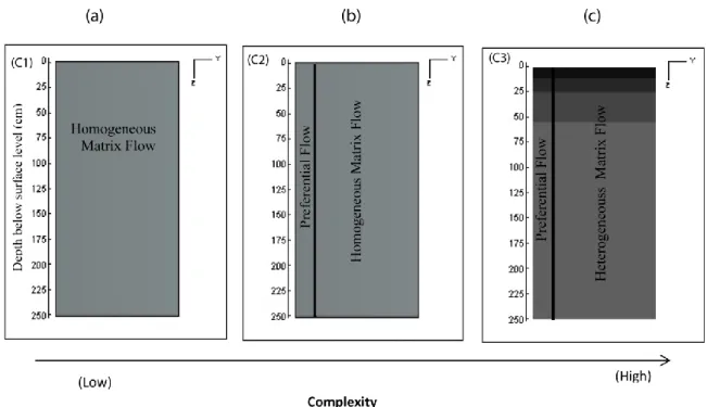
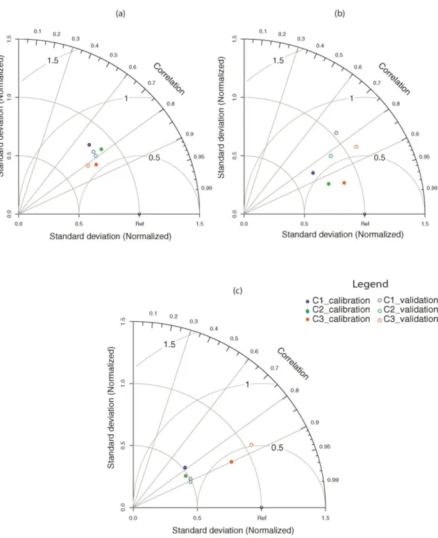
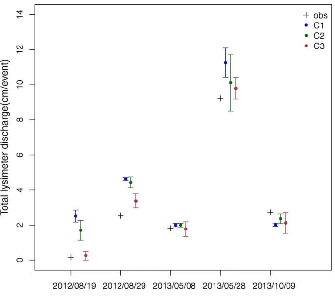
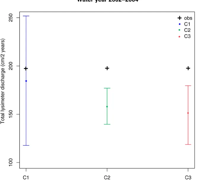
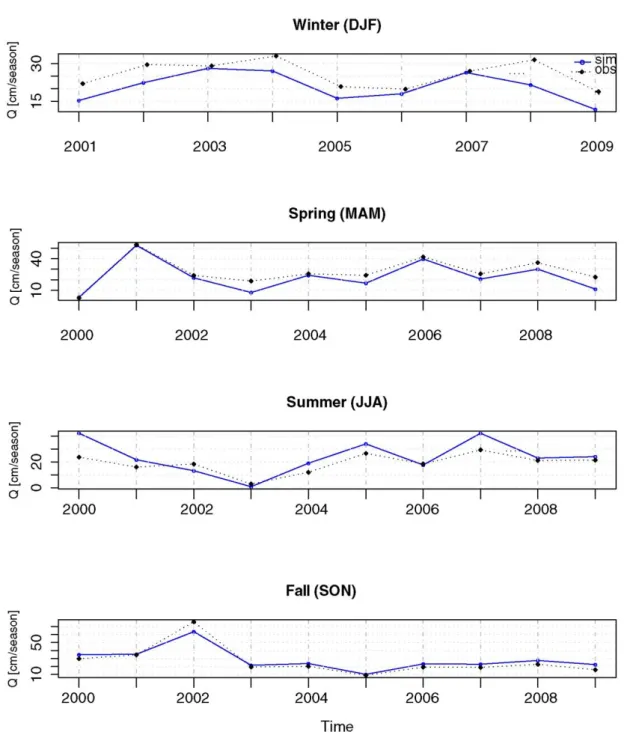
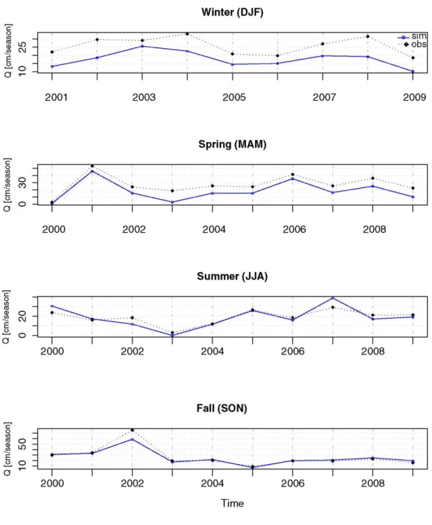
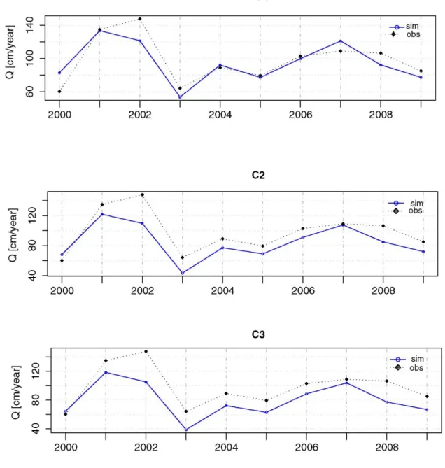
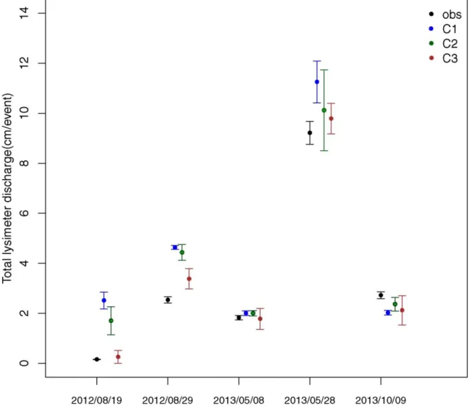
Figure 2-1. Relationship between model complexity, data availability and model performance from Grayson and Blöschl (2001). ... 23 Figure 3-1. Conceptual model setups with different levels of complexity in a vertical cross-section of the lysimeter. (C1) is conceptual model 1 with 7 parameters and only consists homogeneous matrix flow, (C2) is conceptual model 2 with 13 parameters with an explicit preferential flow component and (C3) is conceptual model 3 with 25 parameters. It includes layering (heterogeneity) and an explicit preferential flow component. ... 29 Figure 3-2. Daily observed versus simulated lysimeter discharge (top), evapotranspiration (middle) and average water content (bottom) from 0 to 80 cm below lysimeter surface for all the three conceptual models (C1, C2, C3) for calibration ( June 9th, 2012 to March 30th, 2013) and validation (March 31st, 2013 to November 22nd, 2013) periods. The selected events (highlighted in gray) indicate the event-based lysimeter discharge simulations for each conceptual model. Snow cover periods are highlighted in pink. The vertical red arrow indicates the March 8th event (refer to the text for more explanation). ... 37 Figure 3-3. Taylor plots for lysimeter discharge (a), evapotranspiration (b) and water content (c) for conceptual models C1 to C3. Different colors indicate different models. The results are shown for calibration (filled circles) and validation (empty circles). ... 38 Figure 3-4. Event-based observed versus simulated lysimeter discharge for conceptual models C1, C2 and C3. The events (shown with grey panels on Figure 3.2a) are selected in a way to include varying rainfall intensities. Error bars indicate the 95% uncertainty bounds. ... 40 Figure 3-5. Total lysimeter discharge for monthly (a) and seasonal (b) time scales versus observed values from October 2002 to June 2005 based on conceptual models C1, C2 and C3. Error bars indicate the 95% confidence intervals. ... 41 Figure 3-6. Total lysimeter discharge versus observed values from October 2002 to October 2004 based on conceptual models of C1, C2 and C3. Error bars indicate the 95% confidence intervals. ... 42 Figure 4-1. Convergence of the estimated sensitivity indices with increasing sample size and 95% confidence bounds. (a) Main (Si) and Total (STi) effects for the parameter 3 (w); (b)
Main (Si) and Total (STi) effects for the parameter 10 (Ks4). Refer to the Table 4-2 to see the
description of parameters. ... 63 Figure 4-2. Time-varying daily sensitivity of the discharge RMSE metric to model parameters within the simulation period, i.e., July 2012 to November 2013; (a) smoothed average water content with a window of 47 days. The dotted line indicates the average of the water content for the hydrologic year of 2012-2013; (b) main effect of model parameters; (c) interaction effect of model parameters; PF, SM and ET show groups of preferential flow, soil matrix and evapotranspiration parameters, respectively. ... 65 Figure 4-3. Time-varying daily sensitivity of the evapotranspiration RMSE metric to model parameters within the simulation period, i.e., July 2012 to November 2013; (a) smoothed average water content with a window of 5 days. The dotted line indicates the average of water content for the hydrologic year of 2012-2013; (b) main effect of model parameters; (c) interaction effect of model parameters; PF, SM and ET show groups of preferential flow, soil matrix and evapotranspiration parameters, respectively. ... 67 Figure 4-4. Time-varying daily sensitivity of the water content RMSE metric to model parameters within the simulation period, i.e., July 2012 to November 2013; (a) smoothed average water content with a window of 35 days. The dotted line indicates the average of water content for the hydrologic year of 2012-2013; (b) main effect of model parameters; (c) interaction effect of model parameters; PF, SM and ET show groups of preferential flow, soil matrix and evapotranspiration parameters, respectively. ... 68 Figure 4-5. Smoothed average water content with a window of 10 days for the simulation period, i.e., July 2012 to November 2013 in addition to the annual average of the water content (the dotted line) for the hydrologic year of 2012-2013 (a). Time-varying daily information content of the discharge RMSE (b), evapotranspiration RMSE (c) and water content RMSE metric (d) for model parameters. PF, SM and ET show groups of preferential flow, soil matrix and evapotranspiration parameters, respectively. ... 70 Figure 4-6. Information content of discharge, evapotranspiration and water content versus (a) main effects (b) interaction effects for all the model parameters for the entire simulation period, i.e., July 2012 to November 2013. ... 72
LIST OF TABLES
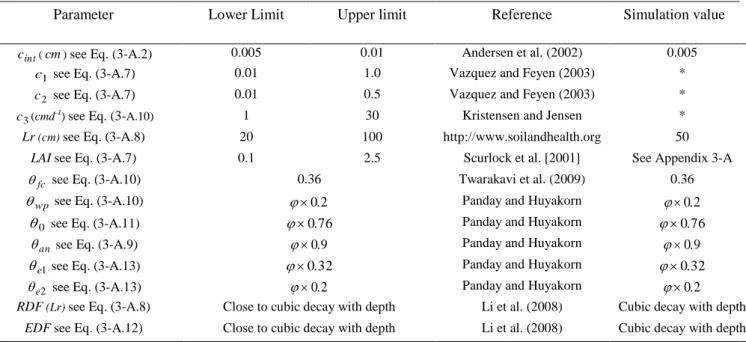
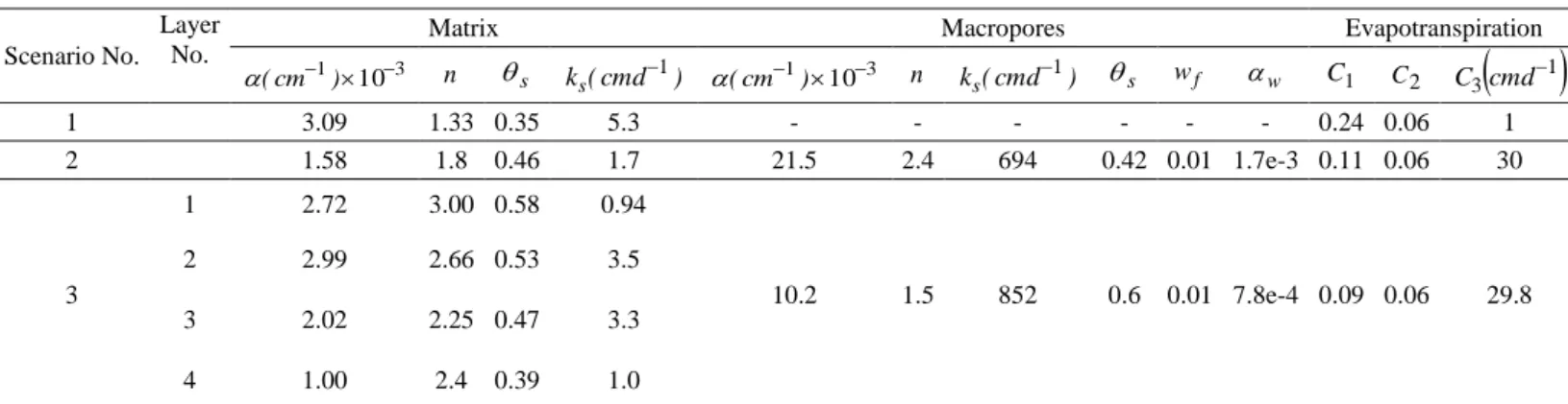
Table 3-1. Evapotranspiration parameters. ... 31 Table 3-2. Unsaturated flow parameters. ... 32 Table 3-3. Calibrated values of the parameters used for the three different conceptual models. ... 36 Table 4-1. Parameters of the model ... 61
1
1
Chapter 1
1.1 Introduction
The proper management of water resources nowadays is a critical issue, not only in lands which suffer from water scarcity but also in countries which are exposed to the risk of high flows. In that sense, accurate measurement of water balance components is a prerequisite for the proper management of water resources since one cannot manage what one cannot measure. Water balance estimates strengthen water management decision-making, by assessing and improving the validity of visions, scenarios and strategies. Therefore, water balance estimation is an important tool to assess the current status and trends in water resources availability in an area over a specific period of time. The water balance equation is a simplistic mass balance equation, in which the difference between inputs and outputs is equivalent to the change in storage of water in the system. The water balance for a given time interval depends upon existing system storage (soil water content) and fluxes from the sides, top (precipitation, runoff and evapotranspiration) and bottom (deep percolation) boundaries of the model domain. In the following, a brief review of the importance and the estimation of those components of a water balance equation which are difficult or cannot be directly measured is given.
Water storage has been shown to be a controlling factor in generating high flows and sustaining base flows in shallow groundwater areas such as headwater catchments. For example, Rinderer et al. (2015) found in a pre-alpine monitoring site in Switzerland that antecedent conditions (storage) were among controlling factors in the response time of groundwater, preceding the peak of streamflow. Penna et al. (2015) found in a similar study in a headwater catchment in the Italian Alps that independent from the geology and land cover settings, the jointly effect of storage in the unsaturated zone and precipitation amount played the dominant role in triggering the piezometric response and total catchment runoff. On the other hand, the influence of water storage in sustaining the base flows have been addressed by many (e.g., Blumstock et al., 2015; Hilberts et al., 2007; Matonse and Kroll, 2013). Tetzlaff and Soulsby (2008) used isotopic and hydro-chemical data and showed the significance of storage in pre-alpine headwater catchments on the quantity and quality of the base flow waters.
2
The change in water storage in a model domain is highly non-linear and has been shown to be highly interacting with other water balance components such as evapotranspiration (Bowling et al., 2003). Evapotranspiration is the sum of evaporation and plant transpiration from the Earth's land surface to the atmosphere. The common approach to estimate actual evapotranspiration (ETa) where direct measurement methods such as eddy covariance are not available is to calculate potential evapotranspiration (ETp). It is the amount of water that would be evaporated and transpired if there were sufficient water available. In that sense, ETp will be adjusted to derive ETa based on the available water and cropped plant. However, this method is uncertain due to the existence of over 50 methods to calculate ETp (Thompson et al., 2014). Vazquez and Feyen (2003) evaluated the effect of three different methods for estimating potential evapotranspiration on effective parameters and performance of the MIKE SHE-code. They found that model performances were comparable and the best model performance was obtained by using the higher ETp values. Bae et al. (2011) used three alternative semi-distributed models and different ETp methods to simulate climate change scenarios in central South Korea. Their results showed that the different ETp methods impacted runoff changes, with the magnitude of ETp-related differences varying between hydrological models and season.
Deep percolation (DP) or recharge, which is the amount of water that infiltrates into the ground, passes the root zone and finally reaches the water table, is the other component of the water budget. DP drives many of the hydrological processes (Bakker et al., 2013) and may provide benefits including: recharging the aquifers, delaying return flow to the streams, diluting contaminants from other sources such as septic tanks. Estimation of DP is often concomitant with uncertainty due to the fact that it is very difficult and costly to measure it directly (Lee et al., 2007). DP is usually estimated via indirect methods such as variations of river streamflow (Combalicer et al., 2008), fluctuation of the water table (Marechal et al., 2006), analytical soil water balance models (Rodriguez-Iturbe et al., 1999) and numerical modeling using Richards’ equation (Carrera-Hernandez et al., 2012).
1.2 Problem description
Due to the difficulty in direct measurements of water balance components, simulation models as useful tools are applied to simulate soil water balance processes (Soldevilla-Martinez et al., 2014; Stumpp and Maloszewski, 2010). With regard to the interaction of the water balance components and the fact that the components themselves are influenced by various factors such as heterogeneity, sub layering, preferential flow paths in addition to hydrodynamic
3
parameters such as field capacity, unsaturated conductivity, antecedent moisture and pore connectivity (Augenstein et al., 2015; Morbidelli et al., 2011; Morbidelli et al., 2014), mechanistic and physically-based models seem to be promising for simulation purposes (e.g., Bolger et al., 2011; Lafond et al., 2014; Rahim et al., 2012). Such models incorporate the affecting factors on water balance components into one framework and help to better understand the involved processes and the time when specific processes become dominant (e.g., Ameli et al., 2015; Cornelissen et al., 2014; Frei et al., 2010). Preferential flow, for example, is one of the processes that the dominant controls on its initiation and its interaction with initial soil moisture are poorly understood (Merdun et al., 2008). In macroporous soils, higher antecedent soil moisture generally increases the depth to which macropore flow penetrates as well as increasing total percolated volume, (Granovsky et al., 1994; Jarvis, 2007). Graham and Lin (2011) analyzed 175 events and found out that initial soil moisture (storage status) was clearly a control on preferential flow initiation. In contrast, Merdun et al. (2008) reported that preferential flow was more evident when soil was initially dry compared to two wetter treatments. Shipitalo and Edwards (1996) also found the relative contribution of
macropores to pesticide transport was greatest when the soil was dry and decreased as the soil became wetter. Nimmo (2012) reviewed preferential flow occurrences and observations in unsaturated conditions and suggested the need for models which do not imply wetter- faster concept. Therefore, one of the main objectives of this thesis is to apply a physically based model and investigate the initiation of preferential flow, its relevance to antecedent moisture condition and its effects on the estimation of evapotranspiration, deep percolation and storage change. Nonetheless, one should note that the outputs of mechanistic and physically-based models could be very uncertain due to the problem of non-uniqueness or parameter equifinality (Beven, 2006). Non-uniqueness happens when model parameters cannot be estimated uniquely and therefore different sets of parameters values lead to similar values of model performance criteria. There are a number of factors that cause the non-uniqueness problem, including the interactions and correlations among the parameters being optimized simultaneously, and the insufficient information content of experimental data used for calibration. Therefore, the other two objectives of this thesis are to; i) investigate different levels of complexity, implying the optimized number of parameters required to represent vadose zone processes and avoid equifinality ii) evaluate the worth of different observation datasets in constraining model parameters and therefore reducing their uncertainty.
In order to accomplish the objectives of this thesis, high quality data of water balance components are required. It goes without saying that an accurate estimation requires accurate
4
measured data for validation. In that sense, weighing lysimeters are appropriate experimental facilities for accurate measurement of soil moisture change, evapotranspiration and deep percolation. Lysimeters have been widely used in hydrological and water balance studies due to:
Measurements: All measurements have limitations in accuracy and one can just expect the
measured data to be the least-biased. Weighing lysimeters provide the opportunity to measure the water balance components such as actual evapotranspiration with high accuracy. In that sense, actual evapotranspiration based on lysimeters measurements have been employed as reference data to evaluate established methods and develop new formulations for estimating actual evapotranspiration (Kashyap and Panda, 2001; Liu and Luo, 2010). In the sense of recharge estimations, lysimeter data have been used as reference to validate recharge estimation methods (e.g., Soldevilla-Martinez et al., 2014; von Freyberg et al., 2015).
Scale: Lysimeters can reproduce field-like conditions. These conditions can be discussed in
terms of the atmospheric boundary conditions and heterogeneity versus homogeneity among soil particles. It is well-accepted in the hydro(geo)logy community that the established formulations, such as Richard’s equation for the simulation of flow in variably saturated medium fail at the field scales (Beven and Germann, 2013; Gerke and Kohne, 2004; Kohne et al., 2006). The reason is that such formulations have been developed under well-controlled boundary conditions in the lab and assume homogeneity among soil particles. Applications of such equations at the lysimeter scale help to understand the limitations of the established formulations under transient conditions and where heterogeneity among soil particles exist. Also, due to the rather small area of a lysimeter in comparison to a catchment, the spatial variation in the precipitation as the model input is negligible.
Wide applicability: The information about evapotranspiration and seepage values which can
be derived from lysimeters have wide applicability for large-scale management of water. For example, Seneviratne et al. (2012) showed that the lysimeter seepage and catchment-wide discharge at monthly scale had a linear correlation of 0.91 based on thirty one years of recorded data. Lysimeters also increase the capability for the cross comparison of results between sites.
In spite of the above-mentioned advantages of using lysimeters in hydrological studies, one should also note the limitations of lysimeters for water balance and hydrological studies. For example, although unsaturated zone drainage from the weighing lysimeters provides the most
5
direct measure of potential recharge, it does not incorporate spatial variability that is contained in watershed-wide estimates of net recharge. Also, the walls of lysimeter casings prevent the latter movement of water from or to the surrounding area. This issue becomes important in the periods of perched water tables. Last but not least is the measurement of runoff which may occur on the top of lysimeters. Usually lysimeters are built, including the one used in this research, with an edge on the top which does not let the collected water on the upper-lying areas to be diverted around the lysimeter.
1.3 Structure of the thesis
This PhD thesis consists of five chapters which address the research objectives stated above. The first chapter starts with introducing the importance of water budget estimation in managing water resources. It continues with a brief review of the methods that are applied to estimate those components of a water balance equation which cannot be or are difficult to measure directly. Consequently, mathematical models as useful tools to simulate water balance components are introduced. In that sense, an elaboration on the advantages and limitations of mechanistic and physically based models is given. To alleviate the limitations of the applicability of such models, lysimeters and their applications in water balance studies are introduced. The chapter comes to an end after outlining a brief review of the contents of the chapters in this thesis.
Chapter two describes the role of subsurface flow dynamics in generating runoff and sustaining the base flow of rivers in shallow groundwater catchments. Application of the tracers methods and simulation models for identification of subsurface flow mechanisms and quantification of subsurface flow contribution to flow generations are addressed. Advantages and limitations of integrated and physically-based models for simulating the water balance components, including subsurface flow dynamics are highlighted in this chapter.
The third Chapter focuses on comparing different levels of complexity for simulating the water balance components in a weighing lysimeter. Three conceptual models, each representing one level of complexity are introduced. In the following, it is described how a targeted calibration of these three models were accomplished and how the calibrated models were compared in terms of their performances. In the end, an assessment of the predictive capability of the three models in reproducing deep percolation at the time scales of rainfall events, months, seasons and years are presented.
6
Chapter four addresses the application of sensitivity and identifiability analyses as two diagnostic tools for better understanding of the complex models behaviors. The main objectives in this chapter are to; i) perform a temporal sensitivity analysis (TSA) to study how the uncertainty in the model output can be apportioned to different inputs, ii) carry out a temporal identifiability analysis (TIA) of model parameters to extract the maximum information content from available observations, and iii) discuss the relationship between TSA and TIA results.
Last chapter comprises two sections. In the first section, a short summary as well as the key findings of the research are described. In the second part, the limitations of the study in addition to some recommendations for future research are presented.
7
2
Chapter2
Subsurface flow contribution in the hydrological cycle: Lessons learned
and challenges ahead - A review
Published in Environmental Earth Sciences Journal
Ghasemizade, M., Schirmer, M., 2013. Subsurface flow contribution in the hydrological cycle: lessons learned and challenges ahead-a review. Environmental Earth Sciences 69(2) 707-718.
Abstract
Subsurface flow to maintain base flow and its contribution to high flow is of high significance. The high contribution of subsurface flow to stream flow has usually been determined based on the application of tracer methods. However, there are some studies that challenge tracer test applications. These studies have shown that tracer test applications lead to a high percentage of subsurface flow contribution since advection and dispersion effects are not individually considered in the mass balance equation. On the other hand, there is not yet a broad consensus of the responsible mechanisms that justify high contributions of underground water to river flows. In this paper, we focus on the contribution of subsurface flow to high flows, although a brief description of their role in low flows is included. We discuss different suggested mechanisms, considering their applicability, strengths and inadequacies. Also, the application of tracer experiments is elaborated. Finally, the challenges of modeling surface/subsurface flow interactions are addressed, followed by a short description of our future targets.
8
2.1 Introduction
Despite the fact that groundwater and surface water are often hydraulically interconnected, they are traditionally considered as two separate systems and are analyzed independently. Such a separation is partly due to the belief that groundwater movement has a much larger timescale than that of free surface water movement, and partly due to the difficulties in measuring and modeling their interactions. There exist extensive hydrodynamic models, with different levels of complexity that treat the surface and subsurface flows independently. Nevertheless, the importance of considering the surface water and groundwater as a single body has become an increasing necessity, in terms of both high flows/peak flows/floods and low flows/base flow (Liang et al., 2007; Weill et al., 2011; Winter et al., 1998). We note that regional/trans-boundary deep groundwater flow is not the focal point of this paper, particularly when we discuss high flows. In fact, the focus is on hillslope areas where groundwater table is shallow. In these areas the unsaturated zone controls the separation of rainfall into surface runoff and infiltration during a rainfall event.
2.1.1 Base flow and low flow
Streams can originate from different sources. The main sources are glaciers, overland flow due to precipitation and subsurface (groundwater) flow. Among these, the latter is the least variable source (Winter, 2007) and therefore the role it plays in terms of sustainability should be considered carefully. This is especially true when groundwater provides a storage mechanism that can help to potentially mitigate negative effects of climate warming on the availability of water resources and maintaining river base flows.
Base flow is defined as the component of flow in a river which is not the direct consequence of the rainfall event but is considered as the outflow of the groundwater reservoir feeding the river during the rainless period (Frohlich et al., 1994). Nevertheless, base flow is typically investigated in the context of rainfall runoff studies in which it is separated from generated stream flow during precipitation. Regarding the importance of base flow in maintaining sustainability, few studies have investigated the involving mechanisms which generate stream flow during inter-storm/seasonal base flow periods (e.g. Kish et al., 2010; Payn et al., 2012). These mechanisms become important when the object is determining base flow (low flow indices) in ungauged catchments (sites). In recent years, problems of droughts have focused attention on base flow periods and the processes sustaining water resources for both human consumption and ecosystem needs during dry spells (Jones et al., 2006b; Lehner et al., 2006).
9
Nonetheless, base flows are often viewed as rather “dull”, static periods compared with more “exciting” flood events. Furthermore, the processes contributing to low flows are often considered to be “simply” groundwater discharges to surface waters. Also, in most cases base flow separation has been accomplished during a rainfall runoff simulation that does not help understanding base flow processes seasonally, particularly when evapotranspiration is high. Additionally, a given system or reach may be losing during high flow/river stage but become gaining as flow declines and the hydraulic gradient shifts toward the channel. Studies have shown that such two-way exchange does occur and that it can impact riparian groundwater and stream flow chemical composition long after floodwaters recede (Baillie et al., 2007; Squillace, 1996; Whitaker, 2000).
In many cases, the majority of stream flow discharge during low flow periods is derived from groundwater storage releases (Smakhtin, 2001). Low flow, as it was defined by the international glossary of hydrology (WMO, 1974) is the “flow of water in a stream during prolonged dry weather”. So, considering groundwater resources as reservoirs that could maintain sustainability as well as knowing how these reservoirs are operating are of great significance. The percentage contribution from groundwater to streams has been reported as high as 60 % by Liu et al. (2004), greater than 75 % by Clow et al. (2003) and up to 80–100 % for snowmelt in three high elevation basins by Huth et al. (2004) [For more examples of the role of groundwater in maintaining base flow, readers are referred to Winter (2007)]. Using a multiple linear regression equation to predict seasonal low flows in Selwyn River in New Zealand, McKerchar and Schmidt (2007) concluded that low flows decreased at a rate of about 32 L/s per year over the 22 years of recording. They attributed this decrease to groundwater abstraction and emphasized as well the role that groundwater could play in maintaining low flow.
To avoid seemingly different interpretations in sustaining stream flow, a distinction should be made between the water that is stored in the soil and moves through the phreatic zone (inter-flow or through-(inter-flow) and deep groundwater. Although there is rich literature on the importance of soil in sustaining base flow seasonally, it is not well documented how soil water interacts with base flow. Maybe the research done by Edlefsen and Bodman (1941), was one of the earliest in the context of soil water dependent base flow. They showed in a plot scale, which was soaked to a depth of 7 m by irrigation and sealed to prevent evaporation, that drainage was continuous over a period of 832 days. Nixon and Lawless (1960) calculated from moisture measurements the downward movement of approximately 28.5 cm of
10
previously stored soil moisture (soil-water) from a 6 m profile of sandy soil during a 6-month dry season. They concluded that slow drainage from unsaturated soil may contribute significantly to groundwater recharge. Remson et al. (1960) indicated through their studies of an intermediate zone at Seabrook, New Jersey, USA, that downward gradients of hydraulic head produced slow but continuous rates of drainage even during the season of evapotranspiration.
Recent studies at the mesoscale (ca. >100 km2) have shown that different parts of catchment landscapes can have markedly contrasting roles in low flow generation (Orr and Carling, 2006; Peters et al., 2006). The aggregated effects of such spatial variation in catchment characteristics are often unclear. For example, using geochemical tracers and hydrometric data, Tetzlaff and Soulsby (2008) showed for a 1849 km2 watershed in Scotland that periods of base flow were very dynamic for sub-catchments of the watershed, based on different reactions of sub catchments to isolated small rainfall events. The issue of diurnal variability in low flows is clearly an issue that warrants further study in order to identify the process controls (Wondzell et al., 2007). Also, there are a few studies which have investigated the nature of interacting controls on low flow generation mechanisms in larger river systems (> 1000 km2). Due to the usual absence of major aquifers in montane headwaters, they are not considered as large contributors of base flow. Therefore, attentions are often shifted to larger groundwater resources in lowland areas as the assumed sources of base flows. According to Shaman et al. (2004) the two limiting factors for lack of enough large-scale studies on controlling factors of low flow generation mechanisms are: 1) absence of tools that allow processes to be extrapolated from point scales to larger catchment scales; 2) downstream increasing anthropogenic impacts in larger catchments and thus, masking natural variability. Tetzlaff and Soulsby (2008) stated that the role of headwater on groundwater in maintaining sustainable downstream low flow is not well recognized in the UK. They also emphasized that base flow generating mechanisms are more complex than what is believed.
Based on what has been explained above, it is clear that further research is needed to understand how base flows sustain water supplies and aquatic ecosystems, if appropriate management is sought to protect these catchment services from environmental change. We believe that better understanding of the interacting controls on low flow generation mechanisms can lead to better management of limited water resources.
11
2.1.2 High flow
The exerted role of subsurface flow has been shown to be of key importance in runoff generation. Pinder and Jones (1969) were among the first scientists who showed the influential contribution of groundwater in runoff through employing a mass balance equation for solutes. They showed that the groundwater component of runoff varied from 32 to 42 percent for three sub basins in the US. To many, it might seem that groundwater movement speed is not fast enough to contribute to runoff generation, but it has been shown, through numerical and experimental studies, that subsurface flow can transmit water at rates sufficient to contribute to storm flow (Fiori et al., 2007; Freeze, 1972; Harr, 1977; Pierson, 1980). Wenninger et al. (2004) showed that subsurface contribution was about 80% during a double peak flood event.
It should be mentioned that when the term subsurface flow is used, it could be the old water (pre-event) already stored in the catchment or new water (event water) that moves underground due to precipitation. Whether the subsurface flow contribution is dominated by old water or new water is still challenging due to different research results. For example, on one hand, Cloke et al. (2006) indicated that pre-event water played a minor role in runoff generation and just in a small number of cases high proportions of old water were observed at the outflow. On the other hand, applying a series of two-dimensional (2D) numerical simulations, Fiori and Russo (2007) concluded that the principal mechanism for stream flow generation in rainfall runoff processes is subsurface flow along the soil-bedrock interface combined with groundwater ridging in the vicinity of the hillslope base. In fact, they determined pre-event water as the dominant discharge contributor to stream flow. This topic is discussed in detail in Section Mechanisms.
It is generally agreed that once rain falls on the land surface, the unsaturated zone controls the separation of rainfall into surface runoff and infiltration. However, how and when the unsaturated zone starts to play this role is under intensive research. Some theories have been suggested from which three of them have been widely accepted. They are subsurface storm flow, variably saturated subsurface flow and partly saturated subsurface flow. These conceptualizations of runoff generation are discussed in details in Section Mechanisms. Generally, it is agreed that if the dominant mechanism is determined or observed, the way for estimating flood features in ungauged catchments is paved. In practical engineering, dominant mechanism or physics-based applications are rarely pursued. Instead, engineers apply a probability distribution model for estimating rare flood events for designing flood control
12
structures. Although this approach is easy to use and may result in good estimations, particularly in catchments which have long flow records, it assumes that future events are similar to those previously observed (stationarity). Also, this method is ill suited to address hydrologic responses to climate or/and land use changes. In summary, knowing peak flow generation mechanisms can lead to estimations which make sense physically and could also be applied in ungauged catchments as well as catchments in which long records of flow data do not exist.
With respect to the studies of high flows, there are two different kinds of challenges. On the one hand, different theories have been suggested to explain the physical responsible mechanisms that convert the subsurface flow into stream discharge (Cloke et al., 2006; Mcdonnell, 1990; Weiler and Naef, 2003). On the other hand, there are studies that challenge the standard application of mass balance equations, which are used as a basis to estimate subsurface flow contribution to stream flow. These equations are believed to lump the advective and dispersive/diffusive fluxes and thereby affect the interpretation of data (Chanat and Hornberger, 2003; Jones et al., 2006a; Park et al., 2011). In the following, we review the two above-mentioned challenges individually and address the research needs in these areas.
2.2 Mechanisms
Subsurface storm flow is defined as “the water that infiltrates through the ground surface, flows laterally toward the stream as unsaturated flow or shallow perched saturated flow and enters the stream through a seepage face that is above the stream flow level and below the line that the water table intersects the bank river” (Freeze, 1974). Freeze (1974) described the terms “interflow” and “base flow” as part of the stream hydrograph that can be attributed to lateral inflow from the subsurface storm flow and groundwater flow, respectively. He divided the responsible mechanisms for runoff generation in an arbitrary classification into two categories: overland flow and subsurface storm flow.
The concept of runoff generation due to overland flow was first discussed by Horton (1933). He showed through some observations and empirical infiltration curves, that runoff happens if the rainfall intensity exceeds the infiltration capacity. Rubin (1966) showed that if unsaturated soil properties, initial soil moisture conditions, and rainfall intensity are known, the infiltration curves can be predicted. He identified rainfall rates greater than the saturated hydraulic conductivity and rainfall duration longer than the time required for soil to become saturated at the surface, as necessary conditions for overland flow generation. However,
13
Freeze (1974) challenged the Hortonian runoff generation mechanism as the dominant mechanism. He inferred that two conditions are required in order to accept Horton concept as a runoff generating mechanism: 1) overland flow is generated when soil becomes saturated from above (the surface) by rainfall; 2) the runoff processes described by Horton are dominated in arid or semi-arid regions where rainfall intensity exceeds soil infiltration rates. Intensive studies in the beginning of the 1970’s, particularly in humid vegetated areas, showed that Horton’s concept could not justify runoff generation since rainfall intensity did/could not exceed infiltration rate in many cases. For example, in regions with sandy or gravelly soils, rainfall could not surpass infiltration rate, yet nearby stream flows increased [the reader is referred to papers by Rawitz et al. (1970) and Hills (1971)]. The overwhelming conclusion of all those studies was that overland flow was a rare occurrence in time and space in humid vegetated basins. So, the incapability/inadequacy of Horton’s concept in describing runoff processes led to two other theories named “partial area contribution” concept (Betson, 1964), and “variable source area/variable saturated flow(VSF)” concept (Dahlke et al., 2012; Hewlett, 1974; Hewlett and Hibbert, 1963). Partial area contribution theory was based on regular overland flow contributions of some fixed parts of the watershed, whereas the concept of VSF assumed an expanding channel network wherein the channels reach out to tap the subsurface flow systems which have overridden their capacity to transmit water beneath the surface (Freeze 1974). The two major differences between these two theories are: 1) contracting/expanding areas in VSF concept are not fixed parts as they are in partial area theory; 2) partial area concept assumes that saturation starts from above, whereas in VSF theory saturation initiates from below.
2.2.1 Capillary fringe
Although the theory of subsurface flow was discussed as one of the likely dominant mechanisms of stream flow generation in early works of Hewlett and Hibbert (1963), and Whipkey (1965), the theory did not get support from researchers until late 70’s and early 80’s due to lack of enough evidence. Sklash and Farvolden (1979) showed through field observations, isotope applications and computer simulations that rapid increase in hydraulic head near streams caused groundwater ridging and was therefore responsible for rapid contributions of soil water to stream flow. Later, Gillham (1984) did a point-scale field experiment in which he showed the effect of the capillary fringe on water table fluctuations. He indicated that constant specific-yield-based prediction of a recharge value led to a number that was about 30 times away from reality. He then concluded that considering specific yield
14
as a constant value to calculate recharge amounts results in tremendous errors, especially in areas where the water table is close to the ground surface. Therefore, he suggested the specific yield to be determined based on water content-pressure head relation (water retention curves) and the depth to the water table. He then expressed the idea of capillarity and specified that near-zero specific yield values are present in capillary fringe. To show the effectiveness of the capillary fringe theory on subsurface contribution, Abdul and Gillham (1984); Abdul and Gillham (1989) designed lab and field experiments. Within their lab experiment, they designed a box 140 cm long, 8 cm wide, 120 cm high and packed it with medium fine sand in a way that the top right level of the sand stood at 108 cm and the left bottom was kept at the level of 80 cm. Throughout the experiment, they maintained the water table at three different depths and applied rainfall at two different (high and low) intensities. Using chloride as a tracer, their experiment results indicated that the discharge of pre-event water to the pipe at the bottom of the slope proceeded event water, especially at early times of stream flow. They attributed the rapid movement of subsurface flow in the box to the capillary effect. Abdul and Gillham (1989) also conducted a field experiment in an area of 18 m × 90 m in a shallow sandy aquifer at Canadian Forces Base Borden, Ontario, Canada. Based on their short interval water table measurements in their heavily instrumented site, they attributed the sharp rise of the water table in the vicinity of the man-made channel, flowing through the middle of the catchment, to capillarity. Their conclusion was very critical as they wrote ''the temporal and spatial variations in the hydraulic-head and water table responses can only be explained by invoking the principles of the capillary fringe''.
Jayatilaka and Gillham (1996) argued that capillarity is a key factor in controlling dynamics of near stream flow and that incorporation of capillary fringe effects in models could improve the representation of runoff processes as well as their enhanced predictive accuracy. Based on this work, they developed their own model named HECNAR. The model was based on the perception that a watershed can be divided into three zones based on their respective storage characteristics. Zone 1 was the area which extended up to a point in which the water table depth equaled the capillary fringe height. Zone 2 was considered the area where soil moisture was between field capacity and residual moisture, independent of the water table depth. Finally, the moisture deficient area, due to evapotranspirational losses, was named zone 3. The assumptions that were made to approximate the physical system included isotropy and homogeneity of porous media, neglecting interception and depressional storages, and ignored water loss owing to evapotranspiration as it was assumed to be small within the duration of an
15
event. They believed that “HECNAR incorporates the high discharge of subsurface water to the stream as a result of increased hydraulic gradient toward the stream”.
McDonnell and Buttle (1998) challenged Jayatilaka and Gillham (1996), regarding the capillary-fringe-induced groundwater-ridging as the major mechanism of pre-event contributions to streams in near stream environments. They suggested alternative mechanisms such as preferential flow. In fact, they based their criticism on the observation of rapid water table responses in the absence of a capillary fringe. We also think that the assumption “water loss due to evapotranspiration could be neglected” in HECNAR contradicts the definition of zone 3. McDonnell and Buttle (1998) inferred that the widespread applicability of groundwater ridging mechanism remains uncertain as rapid pre-event contributions to storm flow can originate from a range of hydrological processes. Moreover, they were confident that a conceptual paradox exists since the capillary fringe height of a soil is usually inversely related to its hydraulic conductivity. Therefore, the greater the tendency for capillary fringe rise, the less likely that rapid Darcian flux of groundwater can occur even with steepened hydraulic gradients in the near stream zone (McDonnell and Buttle, 1998; Zaltsberg, 1986). Cloke et al. (2006) took the laboratory experiment of Abdul and Gillham (1989) to validate the hypothesis of capillary fringe effect on pre-event contributions within a 2D finite element numerical model. They showed that while the ridge has not yet reached the surface, Darcian velocity vectors move away from, rather than toward, the channel to fill the area of storage in the unsaturated zone. In fact, they indicated through their simulation results that the ridge formation was not responsible for the pre-event contribution to the stream as the pre-event contribution started to begin when the surface pressure head equaled to zero. Afterwards, they showed the low proportion of pre-event water contribution to stream discharge, which was hypothesized to be due to groundwater ridging in specific conditions of the Abdul and Gillham (1984) laboratory experiment. They varied some influential variables and carried out a set of numerical simulations to look for evidence of groundwater ridging mechanism and pre-event contributions in other conditions. The variables which they varied were, initial water table depth, rainfall intensity, slope, saturated hydraulic conductivity, capillary fringe height, and volume of the sand box. It is beyond the scope of this paper to discuss the effects of individual and interrelated variables, however, the main findings of their numerical experiments were as follow:
16
1) Rainfall intensity was the most sensitive variable which influenced the portion of pre-event contribution, though its effect in ridge formation was limited to high hydraulically conductive areas where the capillary fringe did not reach the ground surface.
2) Whereas the capillary fringe was seen to be a controlling factor in ridge development, it had little effect on the pre-event water contribution.
3) Initial water table height had the maximum effect on both ridge development and domination of pre-event water discharge.
Park et al. (2011) also applied a numerical model to a simple catchment and concluded that capillarity cannot lead to enough mechanical flow. Based on the above discussion, groundwater ridging (capillarity), which has been debated over the last three decades, could not be relied on as an influential mechanism to explain subsurface flow contribution to runoff generation. We briefly review two other widely expected mechanisms in the following.
2.2.2 Pressure wave translatory flow
The mechanism is very analogues to variable saturated flow as it suggests that some subsurface layers will be saturated temporally and will extend in area and volume across slopes or large parts of catchments. Compared to the VSF mechanism, however, pressure wave translatory flow will initiate when continuous hydraulic connection is established across slopes and elevation zones, and thus individual groundwater bodies link together (Becker, 2005). Burt and Butcher (1985) provided evidence to show the applicability of this mechanism by observing groundwater level fluctuation in a densely instrumented 1.4 ha hillslope in UK. They observed that as soon as previously disconnected groundwater bodies at bedrock interface merged and formed a continuous saturation layer across the slope, a secondary rise in stream flow occurred. Similar observations were reported in other catchments (Bazemore et al., 1994; Becker, 2005; Kirnbauer and Haas, 1998; Torres et al., 1998). Although the mechanism seems to be logical and it makes sense physically, experimental evidence on this kind of subsurface runoff and the conditions that control it are poorly understood. Also, quantifying different components of this perceptual model has not been widely done. For the most recent applications of pressure wave theory, readers are referred to Vidon (2012).
17
2.2.3 Transmissivity feedback
The mechanism is based on the idea that saturated hydraulic conductivity decreases as depth increases. In fact, transmissivity feedback is a special case of translatory flow where shallow groundwater displacement is enhanced by a decrease in saturated hydraulic conductivity with depth (Uhlenbrook and Hoeg, 2003). This mechanism was first introduced by Bishop (1991) and since then it has been widely applied in the field of hillslope runoff generation. Cloke et al. (2006), for example, incorporated the method in a numerical experiment to test its applicability in explaining high amounts of observed pre-event water. They concluded that even though the water table levels rose rapidly, less stored (old/pre-event water) water was enabled as discharge due to decreased hydraulic conductivity (potential water movement). Bishop et al. (2011) described runoff response and quantified total water storage, flow paths, and vertical distribution of lateral flow in a catchment of 6300 m2, using the principles of the transmissivity feedback runoff generation mechanism. [For more applications of transmissivity in runoff generation, readers are referred to Kendall et al. (1999); Laudon et al. (2004); Detty and McGuire (2010) ].
This variety of interacting processes, found in different environments, makes the estimation of how water enters the stream at a given site problematic without field investigations. We strongly believe that there is not yet a broad consensus on how subsurface flow contributes to stream flow, even in one specific catchment or site. It goes without saying that first-order controls in one catchment may not be controlling factors in other catchments, depending on variation in geology, soil properties, rainfall features (duration and intensity), geometry, land use, etc. [for a review of how above-mentioned factors may affect stream flow generation, readers are referred to Bachmair and Weiler (2011)]. It seems that state variables are promising for generalization to similar catchments. Weiler and McDonnell (2004) argued that documenting idiosyncrasies of new hillslope environments should be replaced with defining generalizable appropriate state variables in different environments. They believe that if this shifting occurs, major experiments and excavations done in a specific hillslope/catchment will have transference value to a neighboring environment as a variety of properties change. Weiler and McDonnell (2004) developed a numerical physically-based model, named HillVi, and explored the variation of drainable porosity as first-order control in hillslope hydrology. They tested their hypothesis (assuming drainable porosity as a first-order control) for a virtual hillslope by application of their model to simulate flow and transport for two different drainable porosity values while keeping other parameters and inputs constant. They concluded
18
that drainable porosity can explain spatial and temporal variation of subsurface flow, saturation depth, tracer movement and its concentration as well.
2.3 Numerical analyses of tracer applications
McGuire et al. (2007) argued that tracer experiments and their resulting breakthrough curves can be counted on as additional data sources which reflect the complexity of physical processes into one signal, like a hydrograph, as well as integrating flow heterogeneity and thus as tools that can constrain parameterization and reduce model uncertainty. Tracers can also delineate the origin of water (Chen et al., 2012). Nevertheless, the incorrect judgment based on their applications could end in misleading results.
In principle, the contribution of pre-event water can be derived based on the results of tracer data, which are interpreted using mass balance equations. The assumption that has been implicitly put into mass balance equations is that hydrodynamic mixing processes (such as mixing of pre-event and event water) are adequately accounted for in the calculation of the volumetric subsurface flow contribution (Jones et al., 2006a). To determine the proportion of event water and pre-event water with application of conservative tracers, it is very common to first sample subsurface water and rainwater to know their respective tracer signatures and then take multiple samples in the stream at regular time intervals during the storm and for a while after it has ended. Afterwards, based on different ratios of concentrations in the stream water and unit hydrograph, the above mentioned proportion will be calculated. The key point about the hydrograph separation done this way is that it can only differentiate sources of water (event/pre-event) and cannot separate between water pathways (Jones et al. 2006a). In fact, there should be a clear distinction between temporal water sources (event/pre-event or old/new) and water flow pathways (overland or subsurface saturated/unsaturated). Renaud et al. (2007) define pre-event water as the water that is stored in a catchment prior to the beginning of a rainfall event. It is very important to note that pre-event water can follow different pathways to contribute to stream flow. Buttle (1994) accounted groundwater as only one out of six processes that can deliver pre-event water. In summary, there seem to be a necessity to scrutinize the efficiency of mass balance equation applications in order to better estimate the percentage of pre-event contribution.
VanderKwaak (1999) applied a finite element method to simulate the rainfall runoff experiment of Abdul and Gillham (1989) relying on a tracer-based separation method similar to that used by Abdul and Gillham (1989). He found significant discrepancy between model
19
results (subsurface contribution) which were obtained when tracer (bromide) concentrations at the outlet were entered into mass balance equations and when nodal tracer fluxes were summed. Whereas he did not explicitly separate advective tracer contributions from dispersive/diffusive contributions to total solute fluxes entering the channel at each time step, he suggested that the discrepancy could have occurred due to dispersive/diffusive mixing processes at the surface subsurface interface. In light of the factors that can affect the strength of hydrodynamic mixing, Jones et al. (2006a) introduced mechanical dispersion, molecular diffusion, and rainfall intensity/duration as the influential factors. They conducted numerical experiments to compare the computed Darcian-based groundwater fluxes contributing to stream flow with estimates of those contributions based on trace-based separations. They found that contributions calculated based on the above two mentioned methods were significantly different. They attributed the difference to the hydrodynamic dispersion of event and pre-event water tracers. It was featured in their study that hydrodynamic mixing processes can dramatically affect estimates of pre-event water contributions based on tracer-based separation method, as well as demonstrating that the actual amount of groundwater contribution was smaller than tracer-based estimated amount even if the mixing processes were weak. Jones et al. (2006a) showed through their numerical simulations that event and unsaturated zone pre-event waters mix with each other by means of dispersive/diffusive processes before discharging into the channel. To further demonstrate the impact of dispersive/diffusive mixing processes on traditional based hydrograph separation, they assessed the influence of subsurface longitudinal dispersion, rainfall/intensity duration and multiple sequential rainfall events. Having increased the value of the dispersion coefficient, they observed a noticeable increase in the estimate of tracer-based pre-event contributions. In contrast, they decreased the coefficient to near zero. Then, the subsurface contribution minimally declined in comparison to the base case. They stated that even though the effect of mechanical mixing was eliminated, molecular diffusion can strongly influence the mixing process. To indicate the influence of rainfall intensity/duration, they set two scenarios. In the first scenario, they increased rainfall intensity and decreased the duration and in the second one they did just the opposite. In both scenarios the volume of rainfall was maintained equal to the base case amount. They concluded that increased rainfall intensity leads to less tracer-based pre-event contribution, as event and pre-event waters have less time to hydro-dynamically mix before being transmitted to the channel. The converse argument was also made regarding the effect of decreased intensity. Finally, they subjected the system to multiple sequential rainfalls separated by a three-day recovery period. They observed that
20
subsurface contribution decreased as it was expected. They attributed the decline to less mixturing of pre-event and event water as progressively more pre-event water would discharge from the system.
It should be noted that the challenging relationship of capillary fringe and pre-event contribution to stream flow was not clearly and explicitly discussed in Jones et al. (2006a). However, Park et al. (2011) later showed that the capillary fringe can accelerate the mixing of event and pre-event water parcels. Renaud et al. (2007) criticized Jones et al. (2006a) for not distinguishing between temporal sources and mechanical carriers of water contributions to stream flow. This issue was then discussed by Park et al. (2011) stating that the tracer technique for hydrograph separation to deduce the temporal origins of water entering a stream is influenced by pure mechanical flow processes. Also, Renaud et al. (2007) challenged Jones et al. for ignoring kinematic dispersion in water molecules as a potential source of error in estimating the pre-event contribution. Therefore, Renaud et al. (2007) stressed that diffusion and dispersion coefficients for water molecules themselves should be accounted for in modeling, in order to represent their travel through the subsurface, as well as parameterizing them based on site characteristics and tracer properties. Park et al. (2011) clarified the arguments of Renaud et al. (2007) and Sudicky et al. (2007) by showing that the “tracer technique for hydrograph separation to deduce the temporal origins of water entering a stream is influenced not only by pure mechanical flow processes, but also by mixing processes induced by potential chemical gradients”.
Using the fully surface/subsurface integrated model of HydroGeoSphere (HGS), Park et al. (2011) analyzed the relationship between the spatial and temporal origins of storm flow in the stream as well as looking into how precipitation influences the flow in the catchment. To accomplish that, two cross sections, parallel (A) and perpendicular (B) to the stream, of a simplified virtual catchment were assumed. To maintain simplicity, they ignored evaporation and transpiration and assumed uniformity and isotropy of hydraulic properties. Regarding the simulation in plane (A), they observed that pre-event discharge increased far greater than the mechanical subsurface flow component as rainfall intensity augmented. They ascribed the strong pre-event stream discharge, often interpreted based on conventional tracer-based hydrograph separations, to added effects of diffusion and mechanical dispersion. As it is generally accepted (e.g., McDonnell 1990; Weiler and Naef 2003) that considering macropores in porous media can explain the high contribution of pre-event water, Park et al. (2011) applied a dual-permeability approach through attributing 1% of the bulk volume a high
21
hydraulic conductivity value to test this hypothesis. While they considered an arbitrary value of 1% as the simulated bulk volume occupied by macropores, results showed that mechanical contribution of subsurface flow increased, whereas their contribution diminished as rainfall intensity rose again due to further mixing. They concluded that “compared to single continuum simulation cases, pre-event water contributes more to the total stream discharge because of enhanced mechanical input of water and because of the enhanced dispersive input to the stream induced by macropores”. In plane (B), perpendicular to the stream, while pre-event unsaturated discharge ratio to saturated portion incremented due to increase in rainfall intensity, the ratio of increase in exfiltration values (mechanical mechanism) did not reconcile. These results led them to the conclusion that “capillary fringe groundwater ridging may not generate enough mechanical flow for observed pre-event discharge, but it may accelerate mixing processes such that more pre-event water discharges to the stream”. They reached the same conclusion in plane (B) as in plane (A) saying that pre-event water contribution by mechanical flow processes to the stream discharge is limited without dispersion. Results of dual-continuum simulation in plane (B) were similar to those derived for plane (A).
2.4 Modeling
Models as useful hypothesis testing tools enable us to study combinations of conditions which have not yet been encountered in field studies or cannot be replicated at field scale (Johansson, 1985). Recently, physically-based models have been vastly utilized to simulate short-term (event-based) and long-term interactions of subsurface surface flow on the premise that such models can account for internal processes and complexities (James et al., 2010; Jones et al., 2008; Mirus et al., 2011) and hence could be applied in ungauged catchments. Assuming the above mentioned assumption is true, the question that quickly follows is: why such models are calibrated? McDonnell et al. (2007) answer this question quoting “…models based on current theories rely on calibration to account for our lack of knowledge of the spatial heterogeneities in landscape properties and to compensate for the lack of understanding of actual processes and process interactions”.
With respect to process understanding, around three decades ago, Dooge (1986) published a paper titled “Looking for hydrologic laws” and asked for new visions in the science of hydrology. Dooge suggested a new framework for developing new theories including: 1) searching for new macroscale laws; 2) developing scaling relations across watershed scales, and 3) upscaling from small-scale theories. It is surprising that after about 26 years, Dooge’s