Mapping Between Different NoSQL Databases

République Algérienne Démocratique et Populaire

Ministère de l’enseignement supérieur et de la recherché scientifique

Université de 8 Mai 1945 – Guelma –

Faculté des Mathématique, d’Informatique et des Sciences de la matière

Département d’Informatique

Mémoire de Fin d’études Master

Filière

:

Informatique

Option:Sciences et Technologie de l’Information et de la Communication

Thème :

Mapping Between Different NoSQL Databases

Octobre 2020

Réalisé par :

 BOUAFIA Ibtissem

Encadré Par :

Acknowledgments

No work would be completed without encouragement, motivation and sacrifice. First and

foremost, most thanks to ALLAH for giving us the strength and health to realize this work,

I am deeply grateful to my esteemed supervisor Dr. AGGOUNE Aïcha who has patiently

guided the production of this work. Special thanks are given to the jury members

Dr.Mehnaoui Zahra and Dr. Madi Leila for accepting to examine my work.

Eventually, special thanks are offered to my best friend Nor El Houda Redjaimia for her

supported me with wise advice, insightful comments and valuable information at various

stages of this work.

Dedication

I dedicate this modest work to the memory of my sympathetic father "Norddine" and the

candle of my life, my adorable mother, thank you for your prayers your help and Support. To

my lovely sisters: Zeyneb, Asma, Chaima, Ikram and Chourouk To all my brothers:

Abdelraouf, Youçef. To my dearest niece Tasnim . To all the members of my family

BOUAFIA and LABADLA. To all my friends with whom I shared the university life

especially my dear friends " Nor El Houda Redjaimia , Nesrine Menai , Saida Souilah". To all

my teachers. To all those who supported me and encouraged me.

Abstract

NoSQL approach represents a new era in data representation and management to allow the definition and manipulation of large data sets, focusing on scalability and availability. The NoSQL data can be modeled in different data models, such as key-value, columnar, document, and graph. In this context, novel opportunities may arise when leveraging the selection of the NoSQL model, which may be more suitable than another for represent ing or handling such data. It seems useful to propose an approach for mapping between different NoSQL databases to ensure data portability and improve data handling as expected.

Our work aims at providing a bidirectional mapping method between document-oriented and columnar-oriented NoSQL databases. We also focused on the use of two principal NoSQL systems: MongoDB document system and Cassandra columnar system.

The proposed method is described through the rule-based algorithm. We define a set of translation rules between database components to map the document-oriented database to the columnar database. Thus, from these rules, we generate the list of inverse translation rules for ensuring the mapping in the other direction.

The proposed method has been validated through experiments, which give a good result.

Résumé

L'approche NoSQL représente une nouvelle ère dans la représentation et la gestion des données pour permettre la définition et la manipulation de grands ensembles de données, en se concentrant sur l'évolutivité et la disponibilité. Les données NoSQL peuvent être modélisées dans différents modèles de données, tels que clé-valeur, colonne, document et graphe. Dans ce contexte, de nouvelles opportunités peuvent se présenter en tirant parti du choix du modèle NoSQL, qui peut être plus approprié qu'un autre pour représenter ou traiter ces données. Il nous a semblé utile de proposer une approche de mappage entre différentes bases de données NoSQL pour assurer la portabilité des données et améliorer le traitement des données comme prévu.

Notre travail vise à fournir une méthode de mappage bidirectionnel entre les bases de données NoSQL orientées document et orientées colonnes. Nous nous sommes également concentrés sur l'utilisation de deux principaux systèmes NoSQL: le système de documents MongoDB et le système en colonnes Cassandra.

La méthode proposée est décrit à travers l’algorithme à base de règle. Nous définissons un ensemble de règles de traduction entre les composants de la base de données pour mapper la base de données orientée document vers la base de données en colonnes. Ainsi, à partir de ces règles, nous produisons la liste des règles de traduction inverse pour assurer le mappage dans l’autre direction.

La méthode proposée a été validée par des expériences, qui donnent un bon résultat.

Mots-clefs: Bases de données NoSQL, Mappage de données, Règles de traduction, Règles de traduction inverse.

Table of Contents

Table of contents………..……….…………..………..

List of figures………….……….…………..………..………..

List of tables…………..……….…………..………...

Abbreviations and Acronyms………...

General Introduction ………..……….…………..………… 1 3 4 5 6

Chapter 01.NoSQL Databases

1. Introduction ………..……….………...…

2. Motivations of the Emergence of NoSQL Data….……….………

3. Definition of NoSQL Data………..………

4. NoSQL Features………..………..………..………. 4.1.NoSQL Vs SQL Features ………... 4.2.CAP theory………... 4.3. BASE Properties ……… 5. NoSQL Categories………...…… 5.1. Key-Value Databases………

5.2. Columnar– Oriented Databases………..…

5.3. Document– Oriented Databases………

5.4. Graph– Oriented Database ………

6. Conclusion……….... 9 9 10 10 10 12 13 13 13 14 15 16 16

Chapter 02. Mapping between NoSQL Databases: Approaches and

Frameworks

1. Introduction………

2. Motivations of Mapping between NoSQL Databases………..………

3. NoSQL Databases Mapping Approaches ………

4. Frameworks for NoSQL Data Mapping………

5. Conclusion………..………… 18 18 18 20 22

Chapter 03. A Bidirectional Mapping Method between Document and

Columnar NoSQL databases.

2. Choosing NoSQL Databases ………

2.1.MongoDB Database ……….……

2.2. Cassandra Database ……….

3. Bidirectional NoSQL Data Mapping Method Database……….…

4. Algorithms of the Data Mapping Method Database………

4.1. Rule-based Algorithm Database ………...

4.2.Extraction MongoDB Algorithm ……….………….

4.3.Extraction Cassandra Algorithm ……….………….

5. Conclusion ……….………….……….………...… 24 24 26 29 32 32 34 36 37

Chapter 04. Implementation

2. Installation and configuration of the used tools………

2.1. MongoDB………...…….. 2.1.1. Installation of MongoDB………....…… 2.1.2. Configuration of MongoDB………..……….…… 2.2. Cassandra………...………..……… 2.2.1. Installation of Cassandra………...…… 2.2.2. Configuration of Cassandra ……….…... 2.3. Anaconda………...………..…… 2.3.1. Installation of Anaconda………....……

2.3.2. Connection of MongoDB and Cassandra with jupyter ………….…

3. Presentation of the MCCM tool………..…….

3.1. Document to Columnar Data Mapping ………...…..

3.2. Columnar to Document Data Mapping ………...…..

4. Evaluation Study………..………. 5. Conclusion ……….………..…... 39 39 39 39 40 41 41 41 44 44 45 46 47 48 49 55

General Conclusion

References

List of Figures

Figure 1.1 - The CAP theorem...

Figure 1.2 - An example of Key-Value database...

Figure1.3 -An example of columnar-oriented database...

Figure 1.4 - An example of Document-oriented database....

Figure 1.5 - An example of Graph-oriented database. ...

Figure 3.1 - Some data of Management_Stock MongoDB database...

Figure 3.2 - Chebotko logical data model of Hotel database...

Figure 3.3- Overview of Bi-directional mapping method...

Figure 4.1 - Installation of MongoDB....

Figure 4.2-MongoDB as a Service...………...………

Figure 4.3- Download apache Common daemon……….………

Figure 4.4- Open the service cassandra.bat. ……….

Figure 4.5 - Installation of Cassandra service. ………..

Figure 4.6-Cassandra service verification. ………...

Figure 4.7-MakeCassandra as a service from command Prompt.………

Figure 4.8-Cassandra CQL Shell.………

Figure 4.9-Installing PyCharm……….

Figure 4.10- Installation of Jupyter Notebook………...

Figure 4.11-Connection of MongoDB and Cassandra to jupyter………...

Figure 4.12-General implementation architecture of MCCM………...………

Figure 4.13-Principal interface of MCCM tool………...

Figure 4.14 -Document to Columnar data mapping.………...

Figure 4.15 -Document-oriented database extraction……………..

Figure 4.16- Result of Doc2Col data mapping…………...

Figure 4.17 - Columnar-oriented database extraction…………

Figure 4.18-Result of Col2Doc data mapping..………..

12 14 15 15 16 25 27 30 40 40 41 42 43 43 43 44 45 45 46 46 47 48 48 49 49 50

List of tables

Table 1.1 - NoSQL databases versus SQL databases……….………….…………..

Table 1.2 -Example of Relational table………...…………..……….…………

Table 2.1 -Comparative study between NoSQL data mapping.…...……..………

Table 3.1- Translation rules of data mapping from MongoDB to Cassandra.……....

Table 4.1- Description of the Management-stock document-oriented database …...

Table4.2 -Queries used in the evaluation study.………….…………..………...

Table 4.3- Similarities between answers for Doc2Col. ………….…………..………

Table 4.4- Description of Cassandra data mapping.………….…………..………

Table 4.5- Description of the Hotel columnar-oriented database………….………..…

Table 4.6-Similarities between answers for Col2Doc. ………….…………..………

11 14 21 31 50 52 53 53 54 54

Abbreviations and Acronyms

Abbreviations Significations

RDBMS Relation database management system

NoSQL Not Only SQL

CAP Consistency, Availability, Partition Tolerance

BASE Basically Available, Soft State, Eventual consistency ACID Atomicity, Consistency, Isolation, and Durability VDPs virtual data partitions

ETL Extract, Transform and Load SDCP Service Delivery Cloud Platform VDPs virtual data partitions

CDPort Cloud Data Portability

CQL Cassandra Query Language

GENERAL INTRODUCTION

1. Context

The NoSQL approach was introduced to deal with the problems of big data, for providing highly scalable systems that are also high performance and highly available. Unliketo relational database, the data stored in the NoSQL are mostly unstructured or semi-structured. Furthermore, the storage of NoSQL data is made in a very flexible way without any constraints or designed schema of data. Hence, the NoSQL system allows the modification of data structure during database usage whenever required due to the schema-less of NoSQL, which is easy to make changes at any time.

Besides, the NoSQL data can be modeled in different data models including key-value model, columnar-oriented model, document-oriented model, and graph-oriented model. Therefore, the data can be stored differently e.g. the document-oriented database stores data in JSON or BSON document formats whereas the columnar database stores data in column structure. Thus, certain NoSQL database may be more suitable than others for representing and handling the data that needs to be used.

2. Problematic

The NoSQL data can be modelled in different data models, where each model has characterized by its data modelling and data handling manner. Some of these models may be more suitable than others for effectively managing the data to be used.

Due to the diversity of NoSQL data model, the possibility of data mapping between different NoSQL databases is highly desirable.

In our work, we focused on the data mapping between two popular NoSQL databases: MongoDB and Cassandra to represent the document-oriented and columnar-oriented databases, respectively.

3. Contribution

This thesis proposes a bidirectional method for the data mapping between MongoDB and Cassandra that allows us to move the same data from MongoDB into Cassandra and vice versa. The proposed method is based on the use of translation rules. We define a set of translation rules between database components to map the document-oriented database to the

columnar database. Thus, from these rules, we deduce the list of inverse translation rules for ensuring the mapping in the other direction.

We also develop a data mapping tool to validate our proposal. The advantages of our data mapping method are multipurpose:

1. It can be used in data integration to extract information from heterogeneous data sources by using a unified model.

2. It involves the data portability and improves data management. 3. It simplifies and automates the process of data transformation.

4. Structure of our master thesis

Our thesis is organized as follows. Chapter 01 introduces an overview of NoSQL data. In chapter 02, we review related work on the mapping between NoSQL databases with a comparison study between different existing frameworks. In chapter03, we propose a method for bidirectional data mapping between MongoDB and Cassandra. Chapter04 presents the implementation of our tool. Finally, we present a general conclusion that resumes the principal contributions with some perspectives for future research.

Chapter 01:

1.

Introduction

The relational databases are considered a vital part that is universally used in information systems. Relational database management system (RDBMS) allows storage, management, and retrieval of varied data. However, the execution of large amounts of data becomes an inefficient process of RDBMS. The non-relational database also known as NoSQL databases have emerged as the solution to manage a large volume of the database, guaranteeing availability, scalability, and partition tolerance.

In this first chapter, we will present the state of the art about the NoSQL databases. Firstly, we describe the NoSQL data with the important motivations of the emergence of NoSQL databases. After that, we outline the principal features of NoSQL such as the CAP theorem, BASE properties, etc. Finally, we will present the different data models for storing and handling the NoSQL data.

2. Motivations of the Emergence of NoSQL Data

Since the appearance of the relational database in 1970, it has taken a big place in the organizational information systems for good storage and manipulation of data using the SQL (Structured Query Language) language. However, over the years certain problems have appeared during the manipulation of these databases, the most important are [1] [2]:

 Volume: the data have become very large that the RDBMS cannot ensure their storage and querying.

 Velocity: data are evolved quickly, which require a lot of time to process.

 Variety: The huge volume of data causes the variety and heterogeneity of data value that the RDBMS needs to use complex data types that are sometimes difficult to express. These data can be structured like a relational database, semi-structured data such as XML documents and non-structured data as images.

 Rigidity of relational database: the relational data were built according to a fixed relational schema. We cannot add new data without filling all the columns of the relational table. In the case of the missing value, we use the special value, well-known Null.

 Limited scalability: relational database is not adapted to the changes of the environment required by the large volume of data; the only solution is to apply a segmentation of relational tables for managing the distributed database, which takes a lot of time and effort.

 Limited distributed processing: the processing of huge volume of data involves using distributed transactions which are often difficult to achieve.

Managing huge quantities of data typically requires the database to be able to scale. A new approach of a database able to present, store, and process these large data, called NoSQL.

3. Definition of NoSQL Data

The NoSQL data have been appeared to store and manage big data that the relational database management systems (RDBMS) cannot handle. There has been no strict definition of NoSQL. The term NoSQL referred to as "Not only SQL" that was first used by Carlo Stozzi in 1998 to represent a huge volume of data, which can be differentially represented from each other [3]. NoSQL data represent an alternative to traditional relational databases in which data are placed in tables and data schema is carefully designed before the database is built. They are especially useful for working with large sets of distributed data [4]. NoSQL began to exploit in China since 2009 [5]. There are over 250 types of NoSQL databases around the world, the some notable systems of NoSQL are MongoDB of 10gen Company, Facebook's Cassandra database, Google's BigTable and Amazon's Dynamo [5]. Compared to the relational database, the data stored in the NoSQL are mostly unstructured or semi-structured. The storage of NoSQL data is made in a very flexible way without any constraints or designed schema of data [6].

Thus, the querying of NoSQL data is faster than in relational databases due to the use of analytical queries rather than the transactional ones. The data can also be managed by parallel processing over different clusters of machines through the MapReduce paradigm [7].

The NoSQL data provide highly scalable systems that are also high performance and highly available[8].

4. NoSQL Features

The NoSQL data are designed to store, process, and analyze extremely large amounts of semi-structured data. We present below the principal features of NoSQL database.

4.1. NoSQLVs SQL Features

The relational databases are not able to store and process a huge amount of data in the distributed environment [9]. A new approach for big data modeling has emerged, so-called NoSQL. In this context, it may be necessary to present the principal features of NoSQL against SQL approach as follows [10-11]:

1) Schemaless: also called dynamic schema or schema-free, which means there is no fixed schema of the NoSQL database to follow like in the relational databases. The

NoSQL schema has more flexible in the data storage without any constraints or designed schema of data.

2) Different data models: unlike to SQL approach where the data must be modeled by the relational model, NoSQL provides four data models: Key-value, wide columnar, document, and graph. Therefore, with these four data models, we also distinguish four types of NoSQL databases.

3) Unacceptable ACID properties: the relational databases strongly follow the ACID transaction properties (Atomicity, Consistency, Isolation, and Durability) while the NoSQL databases follow BASE (Basically Available, Soft State, Eventual consistency) properties.

4) Auto-Sharding with replication: allows the workload to automatically spread across any number of servers in distributed environments.

5) High Availability: the NoSQL approach ensures the availability of a large data in the distributed environment with a high scalability, which means the possibility of adding new nodes without any problem.

6) Simple API: NoSQL data management is done through object-oriented APIs. The following table illustrates a comparison between NoSQL and SQL databases: [

Features NoSQL database SQL database

Data size Large-scale data Size ≤128 terabytes.

Data structure Unstructured or semi- structured data

Structured data (tables)

Data type Various data type Homogeneous data type

Scalability Easy scalable without costs Scalable with high cost

Availability High available Available with high cost

Consistency Difficult to achieve High consistent Partition tolerance High tolerant Less partition tolerant

Query complexity Simple queries More complex

Data schema Schema less Rigid schema

Data model Different data models Relational model Table 1.1 - NoSQL databases versus SQL databases.

4.2. CAP theory

The CAP Theorem, also called Brewer’s Theorem was posited by Eric Brewer in 1998 and codified into a formal theorem when its proof was published in 2002 by Nancy Lynch and Seth Gilbert [13]. Typically, the CAP theorem is applied in the distributed environment, where the performance of the distributed database is related to the consistency of data, the availability of data in the network, and the partition tolerant. These three properties are known by the CAP theorem properties.

 Consistency: All nodes in the network exactly see the same data, even when there are updates.

 Availability: whatever the system used the data must always be available by duplicating the data on different notes.

 Partition Tolerance: The ability of a system to cope with the dynamic addition and removal of nodes that are considered a clean network partition that must be able to operate autonomously.

Figure 1.1 - The CAP theorem. [14].

The CAP theorem is the idea that a distributed architecture is not able to provide partition tolerance, consistency and availability at the same time. Only, two CAP properties must be ensured. The theorem proposes that when a network has been partitioned to ensure that a network failure will not prevent communication between servers, the distributed system must choose between consistency and availability [15]. Generally, the distributed relational

databases respect the two first properties (consistency and availability), whereas NoSQL databases ensure the two last properties (availability and partition tolerance).

4.3. BASE properties

We remember that NoSQL systems do not have all ACID properties for processing the big data. The NoSQL approach requires different characteristics to enable flexibility and scalability. These opposing characteristics are cleverly captured in the acronym BASE for Basically Available, Soft State, and Eventual consistency. So, BASE consists of three principles properties [16]:

 Basically Available: the system ensures the availability of data even if some nodes of it are unreachable.

 Soft state: Stores don’t have to be write-consistent, nor do different replicas have to be mutually consistent all the time.

 Eventual Consistency: the system will eventually become consistent once it stops receiving input.

The BASE properties accept temporary database inconsistencies, but it is certainly a flexible alternative to the ACID properties for databases that are large scale, containing various types of data.

5. NoSQL categories

In contrast to the relational database that founded on the relational model, the NoSQL data can be modeled in different data models such as Key-value, Document, Columnar, and Graph [17-19]. As a result, according to these data models, we can distinguish four categories of NoSQL databases.

5.1.

Key-Value Database

This category is known by its simplicity, indeed, it is based on the principle of the couple (key/value), where the key represents the unique data and the value is the data of any type. The querying of key-value databases can achieve low latency as well as high performance. However, if a system claims more complex operations, this data model is not powerful enough.

Generally, the Key-value databases are used in the areas of e-commerce, log file management, fraud detection, etc. Examples of key-value systems: Riak, Redis, Aerospike, Oracle NoSQL Database, Oracle Berkeley DB, Amazon, Dynamo and Voldemort.

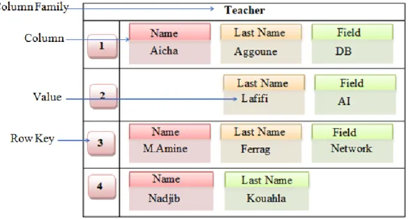
For understanding the structure of each NoSQL database, we take the following relational table which describes some information about a teacher (see table 1.2).

ID Name Last Name Field

1 Aicha Aggoune DB

2 NULL Lafifi AI

3 M.Amine Ferrag Network

4 Nadjib Kouahla NULL

Table 1.2- Example of Relational table

The key-value database corresponds to the about relational table is represented by the following figure.

Key

Value

Figure 1.2 - An example of Key-Value database

5.2. Columnar-oriented Databases

The data are represented by a key row as an identifier and a set of columns described the same topic, which constitutes the column family [19]. When a column contains other columns, we say that this column is a super column. The different column families might be distributed on several nodes. This model is usually used for an efficient storage and processing of a huge amount of tables with a high partition data over several machines. It is more suitable for accounting, averaging, and stock management. The columnar databases do not aggregate all data from each row, but instead values of the same column family and from the same row [20]. The most used columnar-oriented systems are Cassandra, HBASE, and Azure Table. Based on the previous example of a teacher table, the columnar-oriented data is presented below.

Last Name: Lafifi Field: AI

Last Name:

Lafifi

Field: AI

Name:M.Amine Last Name: Ferrag Field: Network

Name: Nadjib Last Name: Kouahla Name :Aicha

Last Name:

Aggoune

Field: DB

Figure 1.3 -An example of columnar-oriented database

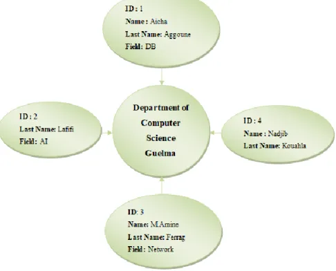
5.3. Document-oriented databases

This NoSQL data category is based on the key/value database, where the value is a document which contains a list of fields. Each field contains a value which can be simple, list of values, document that called embedded document, list of documents, reference or list of references to other documents. The structure of this category is described as follows. [20]

 Collection: a set of documents of the same type. It is equivalent to relational table.

 Document: a set of fields or attributes with their values. It is equivalent to the tuple.

 Key: designed by _id. It is a unique identifier for each document. The following figure illustrates the structure of document-oriented data.

Figure 1.4- An example of Document-oriented database.

{ "_id": 1, "Name":"Aicha", "Last Name": "Aggoune", "Field" : "DB" } { "-id": 2, "Last Name ": "lafifi", "Field": "AI" } { "_id": 3, "Name":"M.Amine" "Last Name": "Ferrag", "Field":"Network" { "_id": 4, "Name": "Nadjib", "Last Name": "Kouahla" } Collection "Teacher"

5.4. Graph-Oriented databases

The data are represented by a graph, where the nodes represent values and the edges defined relationships between different nodes. The graph-oriented stores are widely used for representing complex data like social and biological networks, data of electronic circuits, and services to establish relationships and properties between multiple values. Hyper GraphDB, AllegroGraph, IBM Graph, and Neo4J are four examples of a graph-oriented system. The Neo4j is the popular graph-oriented system because it offers transaction properties, so-called ACID (atomic, consistency, isolation, and durability) [11].

Figure 1.5 -An example of Graph-oriented database.

6. Conclusion

NoSQL is an approach that offers an alternative to handle large volumes of data. We have presented the different concepts and properties of NoSQL databases. With the diversity of NoSQL database models, it may be necessary to propose a method for mapping between NoSQL databases. Consequently, in the next chapter, we will review the existing approaches and frameworks for mapping between NoSQL databases.

Chapter 02:

Mapping between NoSQL

databases : Approaches and

1. Introduction

NoSQL databases have emerged to handle large data sets, which are heterogeneous and arrived at high frequency. They allow the storage and processing of massive data in a distributed environment, ensuring high availability, scalability, and fault-tolerance. Unlike the relational databases, where the data have modelled through the relational model, the NoSQL databases provide four data models that are different from one another (key-value, Columnar, Document, and Graph). In this context, novel opportunities may arise when leveraging the selection of the NoSQL database, which may be more suitable than another for representing such a large amount of data. This chapter presents the literature review on the topic of mapping between NoSQL databases with different existing frameworks.

2. Motivations of Mapping between NoSQL Databases

We remember that the NoSQL data can be modelled in different data models including, key-value model, columnar-oriented model, document-oriented model, and graph-oriented model [21]. Each data model has characterized by its data modelling and data handling manner. We can identify the following motivations for mapping between NoSQL databases:

1. Some of NoSQL databases may be more suitable than another for representing the data that needs to use.

2. The appropriate NoSQL database can enhance the executing low-latency queries and reduce the cost against other databases.

3. The dissatisfaction of the old database in terms of data querying and data optimization. 4. The need to provide data portability allows us to apply a technique of data mapping. 5. The need for a better alternative to manage a NoSQL database and use business or

technology strategy in a good case involves thinking about mapping data rather than creating a new database from scratch.

Mapping to a new format of data is a suitable solution for getting more information about specific data.

3. NoSQL Databases Mapping Approaches

In this section, we present grounding research about the NoSQL data mapping approaches. Shirazi et al [22] have proposed a design pattern-based approach for bidirection mapping between column-oriented database and graph-oriented database. The design pattern is a solution to common problems in software design. This data mapping approach is used to

provide data portability in the cloud environment, which means the ability to move data and applications from one cloud provider to another. The principle idea of this approach is to define two design patterns. The first one aims to ensure the mapping of the column-oriented database to the graph-oriented database. The second one aims to map the data in the other direction. The approach has applied in the healthcare domain, and the results show that the graph-oriented database is more suitable for representing the complexity data than the column-oriented database, which is more convenient for maintaining data in large size. The approach gives a better result when we need to transform the graph-oriented database to a column-oriented database. Nevertheless, the mapping in the other direction poses some problems related to the amount of data.

Scavuzzo et al. [23] have proposed a meta-model approach for mapping between two specific columnar systems, which are Google App Engine Datastore, and Microsoft Windows Azure Tables. The meta-model is an intermediate model between the source model and the target model. It is, based on the BigTable data model, which provides support for columnar databases. This approach is based on a set of extractors, translators, and inverse translators, where the extractors extract data from the source database and pass them to translators, which in turn, transform them into the meta-model format. The translators pass the data modeled by the meta-model to inverse translators, which are in charge for transforming them into a destination database format. This approach has evaluated using data stored by an application called Meeting in the Cloud (MIC), and the results show that the extraction and conversion time is less than the 0.1% of the time needed for the complete mapping. It also allows developers to easily add new columnar databases, but it is not guaranteed on the one hand, that all portions of data from the source database have been translated, and on the other hand, it takes a considerable overall mapping time.

In 2016, Scavuzzo et al. [24] have enhanced their previous work, by supporting fault tolerance in the mapping of huge amounts of columnar databases. The enhanced approach offers a virtual data partitions (VDPs) of the source database to provide a set of parallel mappings of VDP rather than the mapping of the complete database. This approach is more efficient than the previous one with a speedup of 25 times without losing data. However, the parallel mapping of VDP can be posed some errors. Other related studies have focused on mapping different NoSQL databases like document, columnar, and graph.

Thalheim and Wang [25] have proposed a general refinement theory for data migration. This proposal is derived from the data warehouse technique, well-known by ETL (Extract,

Transform, and Load), and applied general refinement theory for data migration. The data sources move from legacy systems into new systems in which data sources have different structures. The refinement theory specified two subclasses of transformations: property-preserving transformations and property-enhancing transformations. To validate this proposal, the authors developed a formal framework and introduced an approach for verifying the efficiency of this proposal.

Bansel et al. [26] have proposed an online compression algorithm approach for mapping between document and graph databases in the cloud environment. This mapping can be achieved directly or indirectly through the intermediate model. The indirect mapping consists of transforming document databases to columnar databases and then to transform them into the graph format. The experimental study is based on the use of two JSON datasets: Core US Fundamental for finance and economic data, and Twitter tweets from November 2012.The results show that the intermediate mapping enhances the read/write efficiency.

Recently, Darko and Neven[27] proposed a semantic web services-based approach for the mapping of data between different cloud storage systems. The authors focused on dealing with the data lock-in problem that causes data mapping with high cost, time and effort.

The data mapping process consists of the intermediate transformation to the OWL format of ontology before the mapping to another cloud provider. These mappings are based on a set of defined transformation rules. The validation of the approach was done by using two cloud customer relationship management (CRM) systems: Zoho CRM and Salesforce. This work provides good solution to map data between cloud providers without the data lock-in problem. Nevertheless, some limitations can be discovered such as the lack of managing the ontology using API operations.

4. Frameworks for NoSQL Data Mapping

The need to mapping between different NoSQL databases involves building frameworks, which are used extensively in practice. The available frameworks have been created to ensure the mapping between NoSQL databases in the cloud environment. CDPort (Cloud Data Portability) framework [28] provides a unified common API for ensuring the portability between different cloud-based NoSQL data. This framework supports Amazon SimpleDB’s key-value data, MongoDB’s document-oriented data, and Google Datastore’s columnar-oriented data. The NoSQL data mapping is based on three adapters one for each NoSQL system. These adapters allow transforming the data. The SDCP (Service Delivery Cloud

Plat-form) [29] represents a middleware infrastructure that uses resources from multiple cloud columnar-oriented databases for mapping between them.

In [26] a NoSQL data Mapping framework has been proposed, which is based on a meta-model and a compression Algorithm. Wijaya and Arman[30] have proposed a general framework, which combines three existing frameworks [22,23,26] to solve the data mapping problem with a different solution, characteristics, and properties. The developed framework includes mapping algorithms, mapping models, and mapping schemes of four NoSQL databases. We focus on these important NoSQL mapping frameworks to establish a comparative study. Framework Criteria Framework of Bansel et al. CDPortFrame-work Framework of Wijaya and Ar-man SDCP Frame-work NoSQL Data-bases Document, Graph, Columnar Key-value, co-lumn, Document Four categories Columnar-oriented databases NoSQL DBMS MongoDB , Azure Table, Neo4j Google Datastore, Amazon SimpleDB, MongoDB MongoDB, Redis Neo4j, Hbase SimpleDB and Azure Table

Dataset Twitter Generic Twitter Generic

Algorithm

MetaModel, Com-pression algorithm

Adapter,

CDPort data mo-del ETL migration Service-based Algorithm Mapping strategies

Direct and In-termediate

Intermediate Direct Direct

Interface - CDPort’s API Nodejs API Java Persistence

API

Table 2.1 - Comparative study between NoSQL data mapping.

NoSQL databases mapping frameworks commonly provide a uniform interface and unified data model for various NoSQL databases. Each framework concerns some NoSQL stores and uses different API and algorithms. The general framework proposed in [31] is composed of existing frameworks to ensure the mapping between the four NoSQL categories.

As a result, we will propose a new system for mapping between these NoSQL stores without using any existing framework or tool. Also, our solution leads to handle the bidirectional conversion between MongoDB and Cassandra databases.

5. Conclusion

In this chapter, we have presented a literature review for mapping between NoSQL databases with a comparison study of different important approaches and frameworks. Several criteria must be taken into consideration, such as the domain of the dataset, the size of the database, and the data complexity. This chapter is intended as a timely introduction to current thinking about the approach of data mapping which will be held in the next chapter.

Chapter 03:

A bidirectional Mapping

Method between Document

And Columnar NoSQL

databases

1. Introduction

In this chapter, we present the conceptual study of our work, which aims to propose a method of bidirectional mapping between document-oriented and columnar-oriented NoSQL databases. To appreciate our method, we present our algorithms like the "extractionMongo" algorithm, the "extractionCassandra" algorithm, and the translation rules-based algorithm. We also define a set of translation rules for transforming the document-oriented database of MongoDB to the columnar-oriented database of Cassandra. According to these rules, we deduce the inverse translation rules for transforming Cassandra to MongoDB databases. This chapter is outlined as follows: we describe the choosing NoSQL databases such as MongoDB and Cassandra. After that, we present our method of bidirectional NoSQL data mapping. Finally, we introduce the different algorithms used in our data mapping method.

2. Choosing NoSQL Databases

Our work aims to propose a method for bi-mapping between two NoSQL databases. Our research focused on two different NoSQL databases, namely: Document-oriented database and columnar database. These databases are the most popular NoSQL databases for storing and managing large amounts of data. To propose such a method, we must first study the features of each NoSQL database. Due to the various available NoSQL database management systems, we choose the MongoDB as a document-oriented database and the Cassandra as a columnar database. The rest of this section briefly describes the principal features of these databases.

2.1. MongoDB database

MongoDB is a document-oriented database management system that was initially released in 2009 [32]. It was developed by 10gen using the C++ programming language. MongoDB stores the data as a document in binary encoded JSON format (BSON). BSON document contains an ordered list of pairs (field name, value) where the value can be simple or complex like embedded document, reference, list, or array. MongoDB is currently being used by MTV networks, GitHub, Foursquare.

The querying of the MongoDB database is achieved by Mongo shell commands, which are expressed in a JSON syntax and send to MongoDB as BSON objects by the database driver. Furthermore, MongoDB is based on the MapReduce paradigm to more express complex queries. There are several important features for high performance and efficient MongoDB database, namely: complex aggregation with the usage of MapReduce for statistical analysis,

indexing over embedded objects, replication to increase read performance of data, and the automatic sharding into shards (partitions or chinks) to provide high scalability of a distributed data [33].

Generally, MongoDB and other NoSQL databases were managed in distributed and cloud environments. The data in MongoDB can be handled under Master-Slave architecture with high availability by the support for the replication [34]. The replica pair architecture provides a high partition tolerance when a salve or a current master of the replica pair fails.

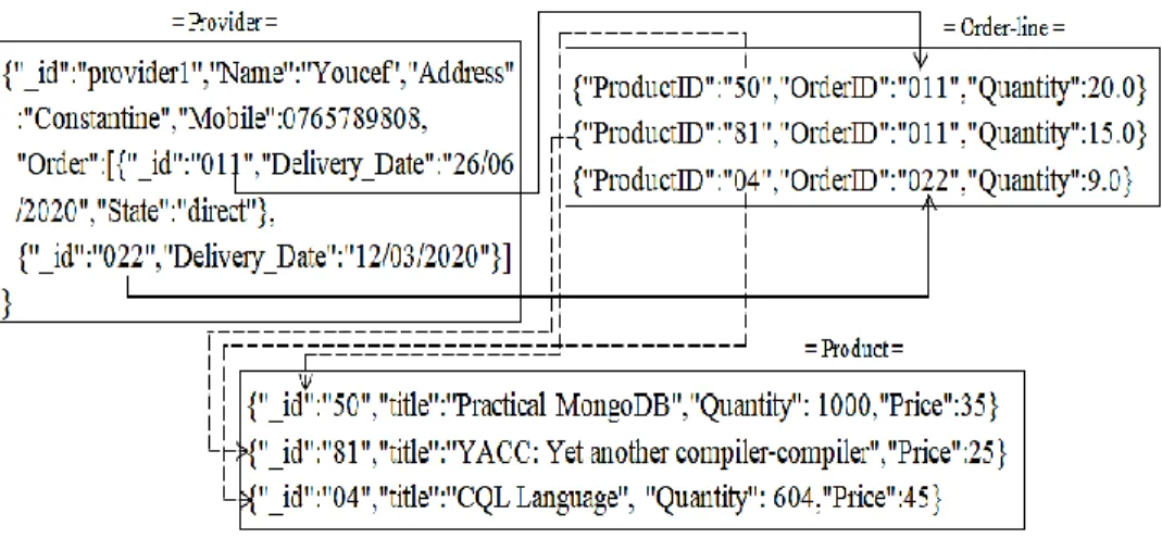
In our work, we have created a MongoDB database for the running example of order management called Management_Stock, which is composed of three collections:

 Provider collection includes the provider’s information with a list of its orders,

 Product describing the information about the product like the title and the price,

 OrderLine collection introduces the relationship between the product and the order.

Due to the schema-less of NoSQL databases, the following figure depicts some data of our Management_Stock MongoDB database.

Figure 3.1 -Some data of Management_Stock MongoDB database

In our database, each provider can offer a list of orders, which is defined by a list of embedded documents. The latter is identified by the identifier of order and can describe the delivery date and the state’s order. Our database contains 1386 documents distributed in three collections as follows: 300 documents in each Provider and Product collections, and OrderLine collection contains 786 documents.

2.2. Cassandra database

Cassandra is a columnar-oriented database management system, which is developed by Apache Software Foundations in 2008 [35]. It is written in JAVA and used Thrift API to data access. Cassandra is a leading transactional distributed database used by Facebook for handling a large amount of data across many commodity servers. It is used by the most popular networking websites like Digg.com, Twitter, and eBay. The Cassandra data storage is very similar to the relational database, made tables, columns, and rows but it does not support join operations between tables. Unlike the relational model, the data of Cassandra are organized in columns rather than rows. Cassandra maps a tuple consisting of a row key, a column name, and a timestamp to a value. Columns are grouped into column families, which are similar to tables in the relational model.

The data model of Cassandra combines the models of columnar Google Big Table and key-value Amazon Dynamo [36]. Further, unlike the MongoDB, Cassandra database uses peer-to-peer replication, namely, Multi-master, providing high availability, scalability with high partition tolerance and persistence. The data are distributed and replicated among several nodes in the cluster, in which the node takes the same role with others (there is no primary or master node) [37]. Cassandra provides two replication strategies: Simple Strategy used when the cluster is deployed across one data center (a group of related nodes), and the Network Topology Strategy, which is used when the cluster deployed across multiple data centers.

To create and manage the Cassandra database, we use Cassandra Query Language (CQL) with the CQLSH driver. Another tool called Data StaxdevCenter provides a graphical user interface to communicate with the Cassandra database [38].

To more represent the Cassandra's database design; we have used one of the data schemas available at the Cassandra’s website (https://cassandra.apache.org). In our study, we focused on the Hotel database schema that describes the general information about the hotel as well as the specific hotels involving hotels near a point of interest, hotels with available rooms, and hotels with available amenities by room. The keyspace of Cassandra database is similar to the relational schema in the relational model. It contains the different column families (also called tables) and the personnel datatypes that are created by a user called user-defined type (UDT).

The UDT can attach multiple data fields each named and typed, to a single column. The keyspace of the choosing database called Hotel, is composed of five column families with a UDT called Address that describes the important fields of address such as street, city, state or

province, postal code, and country. The column families of Hotel keyspace are defined as follows:

- Hotels describes the information about the hotel,

- Hotels_by_poi is used to display a list of hotels near to the point of interest. - Available_rooms_by_hotels_date helps the user to find available rooms. - Pois_by_hotels is used to access the details of each point of interest.

- Amenities_by_room allows the user to view amenities for the desired stay dates.

The Hotel database is defined by the application of the most frequently executed queries to enable the user to easily manage huge amounts of data. To represent the database schema design, we use the Chebotko diagram, which is a novel visualization technique for big data modeling, popularized by Artem Chebotko that represents logical and physical data models by introducing a query-driven application workflow transitions. The logical data model is derived from the conceptual data model with the application workflow, while the physical data model is derived from the logical data model after specifying CQL data types for all columns. Chebotko diagrams compared to the traditional data modeling, improve overall readability, superior intelligibility for complex data models, and better expressivity of both Cassandra schema and queries [39].

Each table of logical model is shown with its title and a list of columns. Primary key columns are identified via symbols such as K for partition key columns, C↑ or C↓ to represent clustering columns , S to represent Static column , IDE to represent Secondary index column, ++ to represent counter column and Lines are shown entering tables or between tables to indicate the queries that each table is designed to support.

The following figure depicts the Chebotko logical data model of Hotel database.

From the above figure,we define the Hotel keyspacein CQL as follows:

CREATE KEYSPACE hotel WITH replication ={‘class’: ‘SimpleStrategy’, ‘replication_factor’: 3}; The Hotel keyspace is based on the simple strategy for replication the data with set to three in the replication factor, which means that three copies of each row, where each copy is on a different node.

The first table (or column family) named "hotels_by_poi", which consists of finding hotels near a point of interest and that by applying the query Q1. This table is identified by a primary key, which is represented by the combination of partition key called poi_name, indicated by the symbol K, and clustering key column sorted by ascending order, named hotel_id, designed by C. It is defined by three other columns: name, phone, and address. The latter is typed through the UDT called Address. The following queries illustrate respectively the creation of hotels_by_poi table and Address UDT.

CREATE TABLE hotel.hotels_by_poi (poi_name text, hotel_id text, name text, phone text, address frozen<address>, PRIMARY KEY ((poi_name), hotel_id) )WITH comment = ‘Q1. Find hotels near given poi’AND CLUSTERING ORDER BY (hotel_id ASC) ;

CREATE TYPE hotel.address (street text, city text, state_or_province text, postal_code text, country text);

The second table called "hotels" consists of getting information about specific hotel and that by applying the query Q2. This table is identified by a primary key called hotel_id and defined by three other columns: name, phone, and address. The following queries illustrate the creation of hotels table.

CREATE TABLE hotel.hotels (id text PRIMARY KEY, name text, phone text, address frozen<address>, pois set<Ttext> ) WITH comment = ‘Q2. Find information about a hotel’; The third table named "pois_by_hotel" describes the points of interest of a specific hotel. This table is identified by a primary key of a hotel hotel_id and clustering key column of point of interest poi_name ordered by ascending order and another column "description" for descripting the point of interest. The following statement illustrates the creation of pois_by_hoteltable.

CREATE TABLE hotel.pois_by_hotel (poi_name text, hotel_id text, description text, PRIMARY KEY ((hotel_id), poi_name) ) WITH comment = ‘Q3. Find pois near a hotel’;

The forth table called "available_rooms_by_hotel_date " consists of finding available rooms by hotel date through the query Q4. This table is identified by a primary key hotel_id and compound of clustering keys columns ordered by ascending order, named (date and

room_number) designed by C. It is defined by another column "is_available" that indicates if the room is available or no. The following query illustrates the creation of available_rooms_by_hotel_date table.

CREATE TABLE hotel.available_rooms_by_hotel_date (hotel_id text, date date, room_number smallint, is_available boolean, PRIMARY KEY ((hotel_id), date, room_number) )WITH

comment = ‘Q4. Find available rooms by hotel date’;

The fifth table named "amenities_by_room" consists of finding amenties for a room that is available for the desired stay dates through the query Q5. This table is identified by a primary key, which is represented by the combination of compound of partition keys called (hotel_id, room_number), and clustering key column ordered by ascending order, named amenity_name. It is defined by another column called description that gives the description of the amenity. The following statement illustrates the creation of amenities_by_room table.

CREATE TABLE hotel.amenities_by_room (hotel_id text, room_number smallint, amenity_name text, description text, PRIMARY KEY ((hotel_id, room_number), amenity_name) ) WITH comment = ‘Q5. Find amenities for a room’;

3. Bi-directional NoSQL data mapping Method

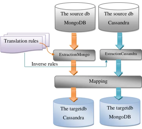
In order to ensure the data portability between different NoSQL databases, we propose a bi-directional mapping method, which is based on a set of translation rules. In fact, we define a set of translation rules between database components to transform the document-oriented database of MongoDB to the columnar database of Cassandra. Thus from these rules, we deduce the list of inverse translation rules for mapping from the Cassandra to MongoDB databases. An overview of our proposal is illustrated in the following figure.

Figure 3.3- Overview of Bi-directional mapping method

The translation rules-based mapping method consists of extracting the components of the source data and applying a set of translation rules for transforming the MongoDB to Cassandra. The translation rule is divided into two parts: the left part defines the concepts of the source model and the right part presents the corresponding concepts of the target model. And from these rules we can deduce the inverse translation rules by inversing the parts of the rule. In the following table, we present the translation rules of data mapping.

Rule Concept of source model (MongoDB)

Concept of target model (Cassandra)

R1 The database name db Keyspace name db

R2 Collection name Table name

R3 Document key of a collection Row key in the table

R4 Index Index

R5 Primary key Row key

R6 View that make a noun to the query result

Materialized view

R7 FieldDocument with atomic value Columnrow with column value The source db MongoDB The targetdb Cassandra ExtractionMongo ExtractionCassandra Mapping The source db Cassandra The targetdb MongoDB Translation rules Inverse rules

F: value F:value R8 Field Document with List of

Values

Columnrow with collection type such as list, set, and map

R9 One embedded document in a document of a collection

Creation of a user-defined-type UDT and used it in the mapped table. R10 List of embedded documents in a

document of a collection

Collection of UDT, like List of UDT and used it in the mapped table. R11 The value of field is a reference to

another document of another collection.

Column has the value of primary key of the corresponding row of another table.

R12 Field has a list of references to other documents of other collections

Column has a list of the values of Primary key of the corresponding row of other tables

Table3.1-Translation rules of data mapping from MongoDB to Cassandra.

From the table above, we are defined the possible translation rules between the MongoDB document-oriented model and Cassandra columnar-oriented model.

The first translation rule R1 consists of using the database name of MongoDB to create the keyspace of Cassandra. This rule is interpreted by the following CQL statements:

ksp_name = print(db.name);

session.execute("CREATE KEYSPACE IF NOT EXISTS %s WITH REPLICATION = {'class': 'SimpleStrategy', 'replication_factor': 1}" % ksp_name)

session.execute('USE %s' % ksp_name)

The second translation rule R2 indicates that all collections of MongoDB database are mapped to the creation of column families (via CREATE TABLE statement).

R3: each document key of the collection C is transformed to the row key of the mapped column family.

R4: the indexes in a collection of MongoDB database corresponds to the indexes in column family of Cassandra database.

R5: the primary key of a collection is mapped to the primary key in the corresponding column family.

R6: each View that make a noun to the query result is mapped to the creation of a materialized view.

R7: FieldDocument with atomic value F: value is mapped to a column definition, where the column name is the same name as the field and the column value is the value of this field. R8: Field Document with a list of values is mapped to a column definition, where the column name is the same name as the field and the column value is the collection of values of this field. This collection type can be the list of values, set of values or map of values.

R9: field has one embedded document is mapped to the creation of user-defined-type UDT used as a type of a column of the mapped column family.

R10: field has a list of embedded documents is mapped to the creation of user-defined-type UDT used in collection type for defining a collection of UDT directly used as a type of the column of the mapped column family.

R11: field has a reference value to another collection’s document is mapped to the creation of column has the value of primary key of the corresponding row of another column family. R12: field has a list of references to other documents is mapped to Column has a list of the values of Primary keys of the corresponding rows of another columns family.

These twelve translation rules can be used for data mapping from Cassandra to MongoDB by inversing their left and right parts.

The mapping method is defined by three algorithms: the "ExtractionMongo" to extract all components of MongoDB, such as collection, document, field, keys, the "extractionCassandra" algorithm for extracting the Cassandra database’s components as column, column family, etc. These algorithms of data extraction are used in the principal data mapping algorithm called rules-based algorithm. We detail the definition of these algorithms in the following section.

4. Algorithms of the Data Mapping Method

We proceed to present the different algorithms that are used for clarifying our data mapping method. The main algorithm of data mapping called rules-based algorithm, which consists in performing the bi-directional mapping between the MongoDB document-oriented database and the Cassandra columnar-oriented database.

4.1. Rule-based Algorithm

The rule-based algorithm is described as follows: Algorithm 1. Rules-based algorithm

Input: SD: source database TR: translation rules

Begin

1. SD Select the NoSQL database to transform 2. If SD is a MongoDB database then

3. Begin

4. Execute ExtractionMongoDB algorithm; 5. Ksp_namedb.name;

6. Create Keyspace Ksp_name; // apply the translation rule R1TR 7. for i in T_Collection[i] do 8. Begin 9. TableNameT_Collection[i].name //apply R2 10. for j=1 to Field.len do 11. Begin 12. Column_name Field[j] 13. Type  get TYPE of Field[j] 14. If Type is atomic then apply R7TR

15. Else if Type is a list of values then apply R8TR

16. Else if Type is an embedded document then apply R9TR 17. Else if Type is a list of embedded documents then apply R10TR 18. Else if Type is a reference then apply R11TR

19. Else if Type is a list of references then apply R12TR 20. End;

21. Extract primary key and apply R5TR

22. Create TableName with column, Type, primary key 23. IndexC=Extract indexes and apply R4TR

24. Index[] Create index indexC on % ksp_name.columF(indexcolumn); 25. InsertData into Table(% column_name , get value)

26. End;

27. Else // SD is a Cassandra database 28. Begin

29. Execute ExtractionCassandra algorithm; 30. dbkeyspace;

31. dbname = Create the database name ; // apply the inverse translation rule R1TR 32. For i=1 to TABLE[n]do

33. Begin

34. T_Collection= create collection with the same names of table TABLE [i] apply the inverse R2TR;

35. For j=1 to COLUMN. len and VALUECOLUMN. Len do 36. Begin

37. Fieldcolumn name ; 38. Valuecolumn value ;

39. Insert into collection the document with the field value 40. T_Collection.create_index(PKEY)

41. End; 42. End.

Output: TD: target database

First, we select the type of the input database: if the database type is a document oriented database then we execute the statements in lines 2-26, else we apply the data mapping from columnar database to document-oriented database (lines 27-40).

In the case of mapping MongoDB to Cassandra, we firstly execute the ExtractionMongoDB algorithm for extracting the components of document-oriented database. After that, we apply the rule R1for creating the keyspace of Cassandra, which takes the name of DB of MongoDB (see lines 4-6), then we apply the rule 2 by copy the names of collection(T_Collection)to another list named TableName (see line 9). For each collection T_collection[i], we store the name of fields and the data types of each document in variables columns, TypeValues, respectively (see lines 12–13). Therefore, we apply the rules R7 until R12according to the data type of the field. After recovering the primary key of a collection, we create the Cassandra table and inserting the data as well as the indexes if they are existed.

In the case of data mapping from Cassandra to MongoDB, we precede the same strategy defined for mapping of MongoDB to Cassandra. After extracting all elements of Cassandra through the ExtractionCassandra algorithm (line 29), we create at the first time, the database db, which takes the same name as the keyspace of Cassandra (apply the inverse rule of R1). Applying the inverse rule of R2, we create collections from the column families (lines 32-35). For each collection, we create the document according to the row and column of column families (lines 35-39). Finally, we add the indexes in each mapped collection.

4.2. ExtractionMongoDB Algorithm

The following algorithm represents how to extract the data and the components of the MongoDB database.

Algorithm 2.ExtractionMongoDB Input: SD: source database Begin

1. X= connection with the selected MongoDB database; 2. db-name = X[the name of the selected database]; 3. T_Collection = extract the collection names; 4. For i=1 to T_Collection.len do

5. Begin

6. Col= T_Collection [i]; 7. Docs= extract all documents;

8. Indexes= Extract all indexes of collections; 9. View= Extract views of the selected collection; 10. Key = Extract all primary keys and their values; 11. For D in Docs Do

12. Begin

13. primary_key [] = Store primary keys into primary_key List ;

14. primarykey_val [] = Store values of primary keys into primarykey_val List; 15. For index in indexes do

16. Begin

18. Indv= Stored all indexes’ values of selected collection into Indv List; 19. End Loop indexes;

20. Item = Extract the pairs (key, value); 21. For it in fieldItem do

22. DocKeys[] =Store fields (also called keys) into DocKeys List; 23. For val in value do

24. Begin

25. if type of val is string or float or int or bool or object then 26. Begin

27. DocValues [] = Store values into DocKeys List;

28. TypeValues[] = Store types of values in TypeValues List; 29. End;

30. Else if type of val is dict then 31. Begin 32. nestedict(val, 1); 33. nestedict(val, 2); 34. nestedict(val, 3); 35. dictpk(val) ; 36. End;

37. Else if type of val is a list then 38. nestedlist(val, 1);

39. nestedlist(val, 2); 40. nestedlist(val, 3);

41. End; //Loop value End; //Loop Docs End; // Loop T_Collection.len

Output:Extracted elements of Data Source

Next, the functions used in the above algorithm Function 1.Nestedict

Def nestedict(dic,numero) :

1. If numer = 1 then store all nested dict keys into dict_keys[] list. 2. Elif numero = 2 then store all nested dict values into dict_values[] list. 3. Elif numer = 3 then store all nested dict types into dict_types=[] list.

Function 2.Nestedlist Def nestedlist(qs,numero) :

1. If numer = 1 then store all nested list keys into keys_list [] list. 2. Elif numero = 2 then store all nested list values into values_list [] list. 3. Elif numer = 3 then store all nested list types into types_list=[] list.

The ExtractionMongoDB algorithm illustrates the data extraction process, which represents the first step of our data mapping method. After the selection of the MongoDB database (line 1) that we need to extract its data and components, we extract the database name as well as the names of all existing collections (see lines 2-3). Then, in the loop from lines 4-10, the algorithm extracts all elements comprising in each collection "Col", such as documents (Docs), indexes, views and keys. For each extracted document D in Docs, we extract both the

column name and the column value of the primary keys (see loop in lines 11-15). We do the same for extracting the information about the indexes (see lines16-20)as well as the fields (lines 21-23).Then, in the loop (lines 36-38), the algorithm verifies if the value of the field is an atomic value, then we store both the value and type in DocValues, TypeValues, respectively (see lines 24-30). In the case where the value of a field is an embedded document, the algorithm calls tow functions: nestedict(val), which extracts all dictionary of keys (values and types) and dictpk(val) for extract all primary keys(lines 31-35).

After that the algorithm analyses if the value of filed is a list of embedded/referenced documents, then it calls the function nestedlist(val) for extracting for each element of the list, their sub elements, such as field name, value (see lines 35-36).

4.3. ExtractionCassandra Algorithm

We give the algorithm for extracting the elements of the columnar databases. Algorithm 2.ExtractionCassandra

Input: SD: source database Begin

1. Keyspace_name = extract the name of the selected database; 2. table_name= extract the table names;

3. for table in table_name do 4. Begin

5. column_name= Extract all columns of tables; 6. views = Extract the materialized views; 7. Indexes = Extract the index_name; 8. for cn in column_name do

9. Begin

10. Column [] = extract the column name; 11. Column_values = Extract the column value; 12. Column_kind = Extract kinds of column;

13. Partition_key = Extract partition keys of a column; 14. clustering = Extract clustering key;

15. Column_type = Extract the data type of a column cn; 16. for t in column_type do

17. Begin

18. UDT[] = Stored type_name extracted into UDT list; 19. Udt-field-name = Extract field_names of UDT; 20. Udt-types = Extract types of fields of UDT; 21. End;

22. End; 23. End; 24. End;