2009/13
Investigation of ventricular cerebrospinal fluid flow phase
differences between the foramina of Monro and the
aqueduct of Sylvius
Phasendifferenzen zwischen den Liquorstro¨mungen im Aqua¨dukt und in
den Foramina Monro
Matthias Schibli1,*, Michael Wyss2, Peter
Boesiger2and Lino Guzzella1
1Department of Mechanical and Process Engineering,
Swiss Federal Institute of Technology (ETH), Zurich, Switzerland
2Institute for Biomedical Engineering, University and
ETH Zurich, Zurich, Switzerland
Abstract
In this paper, phase contrast magnetic resonance flow measurements of the foramina of Monro and the aque-duct of Sylvius of seven healthy volunteers are pre-sented. Peak volume flow rates are of the order of 150 mm3/s for the aqueduct of Sylvius and for the
fora-mina of Monro. The temporal shift between these volume flows is analyzed with a high-resolution cross-correlation scheme which reveals high subject-specific phase differ-ences. Repeated measurements show the invariability of the phase differences over time for each volunteer. The phase differences as a fraction of one period range from -0.0537 to 0.0820. A mathematical model of the pressure dynamics is presented. The model features one lumped compartment per ventricle. The driving force of the cer-ebrospinal fluid is modeled through pulsating choroid plexus. The model includes variations of the distribution of the choroid plexus between the ventricles. The pro-posed model is able to reproduce the measured phase differences with a very small (5%) variation of the distri-bution of the choroid plexus between the ventricles and, therefore, supports the theory that the choroid plexus drives the cerebrospinal fluid motion.
Keywords: choroid plexus; magnetic resonance;
math-ematical model.
Zusammenfassung
In diesem Artikel vergleichen wir Flussmessungen an den Foramina Monro und dem Aqua¨dukt von mehreren (sieben) gesunden Probanden. Die Messungen wurden mittels Phasenkontrast-Magnetresonanztomographie erstellt. Die Volumenstro¨me erreichen sowohl im Aqua¨-dukt als auch in den Foramina Monro Werte von
*Corresponding author: Matthias Schibli, IMRT, ETH Zurich, 8092 Zurich, Switzerland
Phone: q41-44-632-49-39 Fax: q41-44-632-11-39 E-mail: [email protected]
150 mm3/s. Die zeitliche Differenz dieser beiden
Volu-menstro¨me wird berechnet. Die Resultate zeigen deutli-che probandenspezifisdeutli-che Unterschiede. Die zeitlideutli-che Differenz als Bruchteil einer Periode variiert zwischen -0.0537 und 0.0820. Ein mathematisches Modell fu¨r die Druckdynamik des Liquors wird hergeleitet, welches annimmt, dass die Bewegung des Liquors durch die Pul-sation des Plexus chorioideus angeregt wird. Die Vertei-lung des Plexus chorioideus auf die verschiedenen Ventrikel wird als probandenspezifisch modelliert. Das dargestellte Modell ist in der Lage, die probanden-spezifischen Phasendifferenzen mittels einer kleinen Var-iation (5%) der Verteilung des Plexus chorioideus zu reproduzieren. Die Resultate sprechen fu¨r die Theorie, dass die Pulsation des Liquors ihren Ursprung im Plexus chorioideus hat.
Schlu¨sselwo¨rter: Magnetresonanztomographie;
Model-lierung; Plexus chorioideus.
Introduction
The cerebrospinal fluid (CSF) is a clear fluid that sur-rounds the central nervous system, but is also contained in the ventricles, hollow compartments within the brain. Several severe and potentially fatal diseases, such as hydrocephalus, normal pressure hydrocephalus or men-ingitis, are closely connected to the CSF, the most prom-inent being hydrocephalus. Many different aspects of the flow of the CSF have been investigated in the past w17x. Still, not all mechanisms are fully understood. Modeling the behavior of the CSF is motivated by the need for a comparably simple description of the system. This description can be studied better or even virtually manip-ulated without the need of a human or animal experi-ment. The attained knowledge could then be used to further improve diagnostics and treatment of the above-mentioned diseases.
In the vast variety of modeling approaches, there has been much debate about how the motion of the CSF is driven. It has been generally accepted (since the work described by Adolph et al. w1x and the references men-tioned in this section) that the motion of the CSF is driven indirectly by the pulsatile pressure of the cranial arteries. Modeling this energy transfer is challenging. First, there is no obvious causal chain or ordered sequence of events. Secondly, access to the energy transfer via measurements is difficult. The motions of the brain tis-sue, ventricle walls, choroid plexus, etc., are very small
and difficult to measure, even with state-of-the-art mag-netic resonance imaging (MRI) methods.
There are three main hypotheses explaining the driving force of the (pulsatile) CSF flow. One of the early attempts at explaining the propulsion is presented in w7x, where a ‘‘thalamic pump’’ is proposed as the origin of the CSF motion. Based on observations of CSF motion, Boulay concludes that the driving force consists of the two thalami squeezing together the third ventricle and thus pumping the CSF.
Other publications w4, 15, 18, 31, 37x claim that the CSF flow is pumped by the oscillating motion of the brain or directly by the displacement of the ventricular walls. This very motion of either tissue must be driven by intra-cranial arteries, both of which suggest that the driving force originates in the intracranial arteries. Brain motion is usually measured via MRI techniques.
The third hypothesis suggests that the CSF is driven by a pulsating choroid plexus w6, 12, 32, 43x. This hypothesis is supported by the fact that the choroid plex-us is highly vascularized.
Current modeling approaches
CSF dynamics research can be categorized mainly into three different approaches, namely in vitro experiments,
in vivo measurements, and in vivo measurements
com-bined with mathematical modeling. The research described in this paper is based on the latter approach. The presented mathematical model, which is based on established modeling approaches including a new exten-sion, proves to reproduce the measurement results.
Mathematical modeling approaches
An appropriate mathematical model of the CSF dynamics is essential for the understanding of the physiology and the pathology of the CSF. For a better understanding of the proposed model, a number of representative models of the great number of approaches published w46x are reviewed. The order of the different categories is not chronological.
A lumped (one compartment for all ventricles) station-ary model was introduced by Guinane w19x and Rekate w38x. This represents the simplest approach. With this stationary model type, only the net flow of the CSF and stationary pressure phenomena can be captured.
Many new aspects can be studied by adding pulsatility to lumped models, including pressure variations within the cardiac cycle w2–4, 11, 12, 14, 24, 29, 34, 35, 37, 43, 44, 48x. A tabular format review of many intracranial pres-sure dynamic models can be found in w46x. The different (temporal) pressure wave phenomena are well explicable. Spatial pressure waves or pulse waves are omitted completely in all lumped-parameter modeling approach-es because of the extremely short wave travel timapproach-es, which are many orders of magnitude smaller than the time constants of the relevant dynamics.
Further refinement of these models by introducing one compartment for each ventricle leads to multi-compart-ment lumped models w32x. These models can capture the transient fluid exchanges between the ventricles,
partic-ularly through the aqueduct of Sylvius or the foramina of Monro.
Computational fluid dynamic (CFD) models w9, 22, 23, 27, 28, 33x, on the other hand, resolve the equations of motion spatially within each ventricle. These models introduce new possibilities for studying the flow phenom-ena resolved spatially and for looking at transport or mixing phenomena, which was impossible with the other models mentioned. The disadvantage of CFD models is their very high computational burden.
In vitro experiments
A completely different approach is based on in vitro experiments of CSF motions w39, 47x. This approach attempts to replicate the CSF dynamics in a suitable phantom which is more accessible to measurements than in a living human being. This approach clearly offers the possibility of using different and often more accurate measuring techniques. The model presented in w39x, for instance, allows access to the fully three-dimensional, time-resolved flow within the third ventricle, using parti-cle-tracking velocimetry with a spatial resolution that is superior to that of current MR velocimetry.
In vivo measurements
Ventriculostomy, radionuclide cisternography and MRI can be used for determining CSF flow. To date, MRI, which is non-invasive, has been the method of choice. Phase-contrast MRI w10x is preferably used for the detec-tion of laminar flow which can be assessed in a tube, such as the aqueduct of Sylvius. To our knowledge, there are only few published results w5, 13, 21x of flow meas-urements in the foramina of Monro, in contrast to the aqueduct of Sylvius, for which many results are pub-lished, e.g. w36, 40, 45x. One reason clearly is the more complicated geometry of the former method. Wagshul et al. w45x have analyzed the flow phase for the prepontine cistern, the aqueduct of Sylvius, and the spinal canal at C-2 level.
In this paper, flow measurements in the foramina of Monro are presented, with results that are different from those published in w13x. The flow measurement data are analyzed together with data obtained from the aqueduct of Sylvius, and the phase difference between these two flows is computed. Data are presented for several volunteers.
Materials and methods
Data acquisition
The CSF flow data presented in this paper was collected with a clinical MRI scanner (1.5 T Achieva MRI system, Philips Healthcare, Best, The Netherlands) from seven healthy volunteers. A balanced fast field echo (FFE) sur-vey scan was used to identify the three regions of inter-est. For each of the three regions, i.e., the aqueduct, the right, and the left foramen of Monro, a multiplanar reformation was performed to plan the phase-contrast through-plane measurements. All areas of interest were
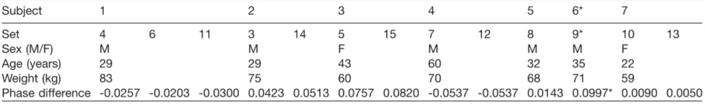
Table 1 Phase differences of all measurement sets of all volunteers as a fraction of one cardiac cycle. Subject 1 2 3 4 5 6* 7 Set 4 6 11 3 14 5 15 7 12 8 9* 10 13 Sex (M/F) M M F M M M F Age (years) 29 29 43 60 32 35 22 Weight (kg) 83 75 60 70 68 71 59 Phase difference -0.0257 -0.0203 -0.0300 0.0423 0.0513 0.0757 0.0820 -0.0537 -0.0537 0.0143 0.0997* 0.0090 0.0050 * Set 9 (subject 6) is dismissed: the volunteer moved during the acquisition.
scanned with the same settings, except for different encoding velocities. Using a view field of 80 mm=80 mm and a slice thickness of 2 mm, a scan resolution of 200=200 leads to a voxel size of 0.4 mm= 0.4 mm=2 mm. A reconstruction matrix of 224=224 achieved by zero-filling of the 200=200 scan matrix before Fourier transformation into the image domain results in pixels in the image domain representing 0.36 mm=0.36 mm of the measured subject. During each cardiac cycle, data on 30 heart phases were acquired. Retrospective cardiac gating was used to ensure an equally spaced coverage of the whole cardiac cycle. A T1-weighted FFE readout with an echo time of 3.8 ms was applied. The acquisition was synchronized retrospectively via a vector ECG trigger on the R-peak. The matrix acquisition was segmented and measured in multiple cardiac cycles. The encoding velocities for the foramina of Monro were 5 cm/s and those for the aque-duct of Sylvius were 15 cm/s. Phase wraps were cor-rected prior to further processing. Depending on the volunteer’s heart rate, the flow acquisition for each region of interest lasted approximately 15 min. Measurements were repeated on different days with the same volunteers for addressing reproducibility issues. One measurement (set 11) was acquired on a different scanner (3T Achieva MRI system, Philips Healthcare). Basic information on the volunteers is given in Table 1.
Post-processing
The cross-sections of the foramina of Monro and the aqueduct of Sylvius have to be defined for each volun-teer individually. The applied semi-automatic segmenta-tion scheme is based on the assumpsegmenta-tion that the power of the desired flow velocity signal is concentrated in the lower frequencies, while the power of the noise is more evenly distributed over the frequency spectrum. In detail, first a temporal Fourier low-pass filter was applied to the measured velocity data, followed by the computation of the variance in time for each voxel reflecting the voxel-based amount of temporal flow variation. A threshold to separate the flow areas, corresponding to CSF, from no-flow areas, which correspond to static tissue, is chosen beforehand for all sets.
The flow in the aqueduct of Sylvius is compared to the flows in the foramina of Monro in terms of phase differ-ences. Therefore, the two distinct flows of the two foram-ina are added and then taken as one volume flow. The phase difference is computed with a high resolution cross-correlation scheme w8x. The cross-correlation is a measure of similarity of two waveforms as a function of a time-lag applied to one of them. First, the flow signal
is up-sampled, which yields more points, and an increased resolution of the cross-correlation scheme. Second, the cross-correlation function itself is interpolat-ed. To test the cross-correlation scheme, the average of the absolute error over various phase shifts is computed using a Monte Carlo simulation. The bases of this anal-ysis are two synthetic sinusoidal flow signals which are deteriorated with a varying fraction of white noise.
Mathematical model
The presented model is a lumped parameter model with one cavity for every ventricle. Every ventricle has a com-pliance with an elastic and dampening part. It is similar to the model proposed by Linninger et al. w32x. Addition-ally, the model is based on the assumption that choroid plexus is distributed in the lateral and in the third ventri-cles. The extension made to that assumption is that the distribution of choroid plexus between the third and the lateral ventricles may differ among subjects.
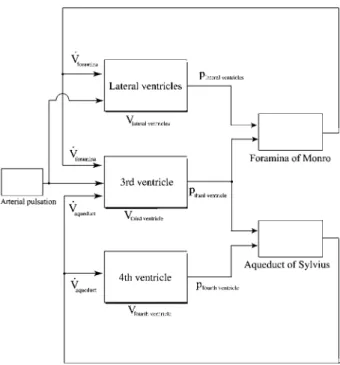
A mechanical analog of the mathematical modeling approach is shown in Figure 1. This model leads to the causality diagram shown in Figure 2. The underlying equations are those of the mass conservation of incom-pressible fluids, yielding:
. . d
Vventr.sV -Vin out
dt
The pressure is computed as follows:
d
pventr.s(Vventr.qVch.plexus)ØEventr.q Vventr.Øcventr.
dt
where Eventr. denotes the elastance (inverse of
compli-ance) of a ventricle and cventr. is the damping constant.
The variable Vventr. is the volume of the corresponding
ventricle. The damping force is assumed to be propor-tional to the rate of the volume change, and hence inhib-iting fast volume changes.
The propulsion by the choroid plexus is modeled as a volume displacement inside the respective ventricles. The varying area of the choroid plexus directly changes the displaced volume since the deviation is assumed to be constant and the volume displacement is modeled as a piston action. The parameters used in the simulation are: total volume of all ventricless20 ml w25x, the relative fraction of volume for each ventricle are 0.864 for the lateral ventricles, 0.0635 for the third ventricle, and 0.0741 for the fourth ventricle. These values are based on the weight of a cast of a human ventricular system. The stiffness of the lateral ventricle is set to 5.53 ml/mm
Figure 1 Mechanical analog modeling of the ventricular system.
The lateral ventricles are lumped together as one cavity, assuming symmetry. Every compartment/ventricle has an elastance and a damping. The choroid plexus drives the fluid motion. Only the pulsating motion is considered.
Figure 2 Causality diagram of the model.
Blocks with shadow represent subsystems with storage (inte-grator) inside. The input is the pulsating pressure in the arteries. The area of the choroid plexus differs from one subject to another.
Figure 3 Frequency spectrum, discrete Fourier transformation
of the flow in the aqueduct of Sylvius (set 11).
Values of the higher harmonics (starting around the 8th) mainly represent the inherent noise of the measurement principle. Note the logarithmic scale.
Figure 4 Semi-automatic area selection to define the lumen.
Right foramen of Monro of subject 1. Background shows a snapshot of the flow rates across the plane at 30% of the car-diac cycle after the R-peak. The circles mark the voxels used to define the volume flow. The measurement plane is normal to the direction of the right foramen of Monro. Flow direction is through plane. Negative flow velocities correspond to a flow into the third ventricle.
Hg w16x and 2.76 ml/mm Hg for the third and the fourth ventricle.
Results
Flow measurements
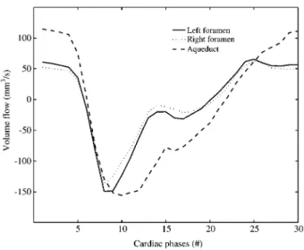
In Figure 3, the spectrum of the flow in the aqueduct of Sylvius is shown. Results of the semi-automatic seg-mentation are shown in Figure 4. In Figure 5, the time-resolved volume flow rates in the aqueduct of Sylvius and the foramina of Monro are shown for a healthy volunteer (set 11). As expected, the flow rates in all ducts are of the same order of magnitude. A slight difference between
Figure 5 Volume flow rates as a function of time of set 11. The volume flow rates of the foramina of Monro are of the same order of magnitude as the flow rates in the aqueduct of Sylvius. Time evolution is slightly different. The measurement is triggered on the R-peak; 30 acquisition frames per period; one time unit corresponds to one acquisition frame.
Figure 6 Phase differences (Dwin fractions of a period) and volume flows of the different subjects.
See also Table 1 for details on the subjects. Subject 6 was excluded; the subject moved during acquisition. The acquisition is triggered on the R-peak; 30 acquisition frames per period; one time unit corresponds to one acquisition frame. Volume flow is in mm3/s. The solid line is the volume flow in the aqueduct of
Sylvius (AQ), the dashed line is the volume flow in the foramina of Monro (FA).
Figure 7 Numerical test of the cross-correlation algorithm.
Cross-correlation error (mean of the absolute error in radian) in function of the available data points per period and the existing noise. Error is computed with a Monte Carlo simulation.
the left and right foramen is visible, which is due to the anatomical asymmetry of the specific volunteer (set 11). The peak velocity in the left foramen is 5.2 cm/s and 5.0 cm/s in the right foramen. These values are signifi-cantly lower than the corresponding values of the velocity in the aqueduct in the same volunteer, which are 10.3 cm/s. A positive flow in the aqueduct of Sylvius cor-responds to a flow into the third ventricle, while a positive flow in the foramina of Monro corresponds to a flow out of the third ventricle into the lateral ventricles. Figure 6 shows flow data of all measurement sets.
Phase differences
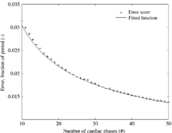
In Figure 7, the cross-correlation scheme is tested with varying fractions of noise and various numbers of samples per period. As shown in Figure 8, the relation between the error and the number of samples per period is inversely proportional to the square root:
, as expected.
1 err;
yNacq
The flow in the aqueduct of Sylvius is compared to the flows in the foramina of Monro in terms of phase differ-ences. Therefore, the two distinct flows of the two fora-mina are added and then taken as one volume flow. Computed phase differences are presented in Table 1 and in Figure 9. A positive value indicates that the flow in the aqueduct of Sylvius is ahead of the flow in the foramina of Monro. Although the phase differences are all rather small, with 5% of a period corresponding to a time lag of 50 ms (at a heart rate of 60 bpm), the values of the phase differences among the volunteers vary significantly. The sign of the phase differences varies as well among the volunteers. In other words, in some vol-unteers, the foraminal flow is ‘‘ahead’’ of the aqueductal flow (negative phase difference), whereas in other vol-unteers the opposite is true. Repeated measurements, with an average of more than 1 month’s time in-between,
Figure 8 Cross-correlation error in function of the available data points per period.
The error is inversely proportional to the square root of the num-ber of data points. The error plotted is calculated using a syn-thetic function with a fraction of noise of 0.145; the fitted function iserrs0.0963.
yNacq.
Figure 9 Phase differences of the subjects. See also Table 1 for details on the subjects.
Figure 10 Relation between variation of area of choroid plexus (CP) vs. phase shift.
Data computed with adapted mathematical multi-compartment model. The sensitivity of the phase difference is strong on the variation of the fraction of choroid plexus. A typical difference among volunteers of 0.3 rad is achieved already at a change of the fraction of 5%.
showed that the phase difference is a subject-specific characteristic.
Mathematical model
The model presented here can reproduce the varying phase differences measured, as shown in Figure 9. Although the inter-volunteer differences of choroid plexus distribution are not tremendous w30x, they are sufficient for explaining the phase differences described above since a shift in the distribution as small as 5% is sufficient to reproduce the typical inter-volunteer differences in the flow phase shift.
As Figure 10 shows, the model with the extension of varying choroid plexus areas is able to perfectly repro-duce the phase shifts measured. To reprorepro-duce the meas-ured phase differences, the distribution of choroid plexus between the two ventricles is only changed slightly.
Discussion
Flow measurements
Only few references on measurements in the foramina of Monro are known to the authors w5, 13, 21x. In w13x, which reports measurement data of several healthy vol-unteers, the peak mean velocity is reported to be in the order of 4 mm/s. The difference of one order of magni-tude between the results shown in w13x and the results presented here may be explained by the very different measurement parameters, the major difference being the slice thickness. In w13x, a slice thickness of 10 mm was used vs. one of 2 mm in our setting. Enzmann and Pelc w13x state that the thickness of the slice leads to partial volume effects since the actual dimension in the anatomy is significantly smaller than their slice thickness. Thus, smaller velocities of surrounding tissue or CSF lead to an underestimation of the actual velocities. These partial volume effects obviously also occur in the measurement plane. This can be observed well in the segmentation of the foramen of Monro in Figure 4 since there is no sharp border between the voxels which would represent the ventricle wall. Some voxels partially represent information on the CSF as well as of the surrounding tissue.
A major factor for attaining repeatable measurements is to design a procedure which is as automatic as pos-sible. The way this is ensured is that only the placement of the measurement planes for the flow measurements are set manually. Due to the plain geometry of the aque-duct of Sylvius, placement is not critical. The direction of the aqueduct is clearly visible on conventional MRI scan protocols, whereas the placement in cranio-caudal direc-tion is of minor importance since the cross-secdirec-tion remains virtually constant over a fair distance. Neverthe-less, the placement of the foraminal measurement planes is more relevant. With the aid of a multiplanar reformation of the survey scan, the position and orientation can be very well anticipated, and hence leading to a consistent
placement of the measurement plane. The segmentation is semi-automated in order to reduce the possibility of human error and to reach a reproducibility which is supe-rior to segmentation by hand. This semi-automated seg-mentation is feasible due to the difference in frequency and amplitude of the flow signal and the noise, see Figure 3.
As described, defining the position of the ventricle walls within the measurement slice, as well as the other steps, do not require any manual adjustment. Repeated measurements were taken with the same volunteer to examine the repeatability. On average, more than 1 month elapsed between the MR scans. Set 11 was even taken on a different scanner (3T Achieva MRI sys-tem, Philips Healthcare) to test for independence. The good agreement among the repeated measurement results is shown in Figure 9.
Phase differences
Applying cross-correlation on the flow data with no fur-ther post-processing, the minimal detectable phase shift would be the length of one sample time dtsTHeartbeatØ 1 ,
Nacq
where THeartbeat is the time for one cardiac cycle and Nacq
is the number of acquired frames per cardiac cycle. With phase differences expected to be smaller than 0.05
THeartbeat, the number of acquisitions per period should be
significantly higher than 20. Currently, the time needed for the readout clearly sets limits to increasing this number. Two different interpolations were used for up-sampling in the time domain. The interpolation of the measured signal is applicable under the assumption that the time evolution of the flow signal is continuous com-pared to the sample time. Figure 5 shows that this con-dition is clearly fulfilled. The resulting high resolution cross-correlation scheme is capable of resolving very small time differences between two functions.
Integrating the flow over the whole cross-section fur-ther improves the signal-to-noise ratio of the flow signal. Partial volume effects are of minor importance for cal-culating the phase differences. The surrounding tissue can be assumed to be static compared to the flow since the amplitudes are in the order of 0.1 mm w42x. The tissue velocities thus can be assumed to be smaller than 1 mm/s. Therefore, even if the movement of the tissue was out of phase compared to the fluid flow, the effect would only be a slightly incorrect value for the magnitude of the vol-ume flow. The phase information would not be affected at all.
The dependence of the signal-to-noise ratio on the number of acquisitions of the MRI scan w20x or the inverse noise-to-signal ratioerr; N
y
acqis proportional to the square root of the number of acquisitions. As the overall error is a product of these two steps involved, the square root of the number of frames per cardiac cycle cancels out. This leads to an error which is independent of the choice of measurement parameters, which are the number of samples per period vs. a better signal-to-noise ratio. The lower limit is given by the Nyquist-Shannon sampling theorem and aliasing considerations (fulfilled, see Figure 3). The upper limit is set by the MRI scan readout time.Since the phase differences are expected to be very small, a rigorous effort is made to ensure that the result-ing values are not affected significantly by noise or gen-eral measurement errors. As a measure of the quality of the overall measurement procedure including post-processing, repeatability is chosen.
It is important to note that set 9 (subject 6) is consid-ered invalid and had to be excluded. The volunteer moved his head during the examination, leading to an insufficient signal-to-noise ratio or a merely recognizable signal.
Mathematical model
The pressure-volume relationship is chosen to be linear. This assumption could easily be relaxed to a non-linear relationship, which would only introduce a function
Eventr.(volume) w11, 41x instead of the constant Eventr.. Since
such an expansion would not change the main results of this paper, the assumption of a linear relation is sufficient. This statement is based on the fact that the general structure of the model would remain the same and the phase differences presented are not only reproducible with the chosen parameters but also with different val-ues. Furthermore, in the pressure range of a healthy vol-unteer, the non-linearity effect is negligibly small. The model presented in this paper focuses on transient and pulsatile effects and can thus reasonably neglect the steady-state production.
The expansion of the choroid plexus is modeled simul-taneously for the lateral ventricles and the third ventricle. This simplification, which is based on the relatively high pulse wave speed in the arteries in the order of 5 m/s w26x, yields only small time delays. It is assumed that this velocity and the corresponding spatial distance remain relatively constant among the volunteers, which corre-sponds to very small inter-volunteer variability of this parameter. The propulsion by the choroid plexus is modeled as a volume displacement inside the respective ventricles. A volume displacement is chosen since the arterial pressure is distinctively higher than the average counteracting intracranial pressure.
Other mathematical models
Different models and their hypotheses on the cause of the pulsatile motion are discussed in the following sec-tion with regard to the flow phase difference variasec-tions measured between the foramina of Monro and the aque-duct of Sylvius.
A rigid wall model, such as most CFD models w9, 22, 23, 27, 28, 33x (the first includes a feet-head motion of the walls, but not in other directions) cannot reproduce any type of phase differences, under the very reasonable premise of an incompressible fluid. With an incompress-ible fluid, a phase difference between the volume flows imposes a change of the volume of the third ventricle during the cardiac cycle. The focus of these models is rather on transport phenomena, where spatially resolved flow information is crucial.
Likewise, models which have only one compartment w2–4, 11, 12, 14, 24, 29, 34, 35, 37, 43, 44, 48x for all ventricles naturally are not able to show such phase
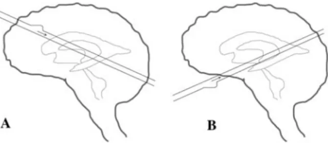
Figure 11 Sketch of how the cerebrospinal fluid may be driven by brain motion to explain the phase differences.
To achieve the change in phase differences with the brain motion, the main arteries would have to lie in a different direction for every volunteer (A vs. B) such that the pressure pulse wave in the artery would hit different ventricles first. See ‘‘Modeling of the driving forces’’ section for an explanation why this is con-sidered infeasible.
differences. But these models stand out with their simplicity.
Multi-compartment lumped-parameter models (more than one compartment for all the ventricles), such as the model presented in w32x, on the other hand, are theoret-ically capable of predicting phase differences. The crucial part in these multi-compartment models is the modeling of the propulsion of the CSF. The different approaches to modeling the propulsion are discussed in terms of their capability of predicting the phase differences.
The multi-compartment in vitro model presented in w39x clearly shows a phase difference. Compared to our measurement results, the phase difference is overesti-mated by the in vitro model. Assuming an incompressible fluid, this leads to the conclusion that the volumetric stiff-ness, often referred to as the inverse of the compliance, was too low in this in vitro model.
Nonetheless, for an exact application of the continuity equation, a summation of all volume flows at every time instance would be necessary. Under the assumption of non-varying cross-sections of the aqueduct of Sylvius and the foramina of Monro, each phase difference in the flows implies a volume change.
Modeling of the driving forces
Using a ‘‘thalamic pump’’ model w7x, the squeezing of the third ventricle would lead to almost concurrent flows out of the third ventricle into the lateral and in the fourth ventricle, in other words causing a phase difference in the order of p. This clearly contradicts our measurement results, which showed almost synchronous flows.
Therefore, we do not see a way to modify this pump mechanism such that it would be able to reproduce our measurement results.
For the hypothesis of the brain motion w4, 15, 18, 31, 37x as the driving force, there are two possibilities of reproducing the measured phase differences with these models. A drastic inter-volunteer difference in the ratio of the compliances between the third and lateral ventricles is one. The other would be an inter-volunteer difference in the anatomical placement of the intracranial arteries, leading to a phase difference in the driving motion itself. As sketched in Figure 11, the traveling pulse wave in the
arteries arrives earlier at one compartment. To switch the order of arrival, the orientation of the main arteries would have to be different. Since neither of these possibilities seems very likely for a variation in healthy volunteers, the phase differences described above are not considered to be explained satisfactorily by this hypothesis.
Conclusion
With measurements of the volume flow in the foramina of Monro and the aqueduct of Sylvius in several volun-teers, we have shown that the magnitude of the volume flow in the foramina of Monro and the aqueduct of Syl-vius are of the same order of magnitude. Peak velocities in the foramina of Monro are smaller than in the aqueduct of Sylvius.
The phase difference between the flows of the aque-duct of Sylvius and the foramina of Monro shows a significant inter-subject variability. The presented mathe-matical model with a propulsion by the choroid plexus is capable of explaining the phase shifts and their vari-ances. Therefore, the measurement results confirm the validity of the model of the propulsion of the CSF via the choroid plexus.
Acknowledgements
We gratefully acknowledge the help of Dr. Michaela Soellinger, Department of Neurology, Medical University of Graz, Austria and Dr. Vartan Kurtcuoglu, Laboratory of Thermodynamics in Emerging Technologies, ETH Zurich, Switzerland as well as the support through SmartShunt – The Hydrocephalus Project of the Swiss National Science Foundation.
References
w1x Adolph RJ, Fukusumi H, Fowler NO. Origin of cerebrospinal fluid pulsations. Am J Physiol 1967; 212: 840–846. w2x Agarwal GC, Berman BM, Stark L. A lumped parameter
model of the cerebrospinal fluid system. IEEE Trans Biomed Eng 1969; 16: 45–53.
w3x Ahearn EP, Randall KT, Charlton JD, Johnson RN. Two com-partment model of the cerebrospinal fluid system for the study of hydrocephalus. Ann Biomed Eng 1987; 15: 467– 484.
w4x Ambarki K, Baledent O, Kongolo G, Bouzerar R, Fall S, Meyer ME. A new lumped-parameter model of cerebrospi-nal hydrodynamics during the cardiac cycle in healthy vol-unteers. IEEE Trans Biomed Eng 2007; 54: 483–491. w5x Bale´dent O, Henry-Feugeas MC, Idy-Peretti I. Cerebrospinal
fluid dynamics and relation with blood flow: a magnetic res-onance study with semiautomated cerebrospinal fluid seg-mentation. Invest Radiol 2001; 36: 368–377.
w6x Bering EA. Choroid plexus and arterial pulsation of cerebro-spinal fluid – demonstration of the choroid plexuses as a cerebrospinal fluid pump. Arch Neurol Psychiatry 1955; 73: 165–172.
w7x Boulay GHD. Pulsatile movements in the CSF pathways. Br J Radiol 1966; 39: 255–262.
w8x Campbell JY, Lo AW, MacKinlay AC. The econometrics of financial markets. Princeton: Princeton University Press, 1997.
w9x Cheng S, Jacobson E, Bilston LE. Models of the pulsatile hydrodynamics of cerebrospinal fluid flow in the normal and abnormal intracranial system. Comput Methods Biomech Biomed Eng 2007; 10: 151–157.
w10x Connor SE, O’Gorman R, Summers P, et al. SPAMM, cine phase contrast imaging and fast spin-echo T2-weighted imaging in the study of intracranial cerebrospinal fluid (CSF) flow. Clin Radiol 2001; 56: 763–772.
w11x Czosnyka M, Czosnyka Z, Momjian S, Pickard JD. Cerebro-spinal fluid dynamics. Physiol Meas 2004; 25: R51–R76. w12x Egnor M, Zheng L, Rosiello A, Gutman F, Davis R. A model
of pulsations in communicating hydrocephalus. Pediatr Neurosurg 2002; 36: 281–303.
w13x Enzmann DR, Pelc NJ. Normal flow patterns of intracranial and spinal cerebrospinal fluid defined with phase-contrast cine MR imaging. Radiology 1991; 178: 467–474.
w14x Fard PJM, Tajvidi MR, Gharibzadeh S. High-pressure hydro-cephalus: a novel analytical modeling approach. J Theoret Biol 2007; 248: 401–410.
w15x Feinberg DA, Mark AS. Human brain motion and cerebro-spinal fluid circulation demonstrated with MR velocity imag-ing. Radiology 1987; 163: 793–799.
w16x Friden H. Hydrodynamics of the cerebrospinal fluid in man. PhD thesis, Umea University. Umea, Sweden 1994. w17x Greitz D. Radiological assessment of hydrocephalus: new
theories and implications for therapy. Neurosurg Rev 2004; 27: 145–165; discussion 166–167.
w18x Greitz D, Wirestam R, Franck A, Nordell B, Thomsen C, Sta˚hlberg F. Pulsatile brain movement and associated hydrodynamics studied by magnetic resonance phase imaging. The Monro-Kellie doctrine revisited. Neuroradio-logy 1992; 34: 370–380.
w19x Guinane JE. An equivalent circuit analysis of cerebrospinal fluid hydrodynamics. Am J Physiol 1972; 223: 425–430. w20x Haacke EM, Brown RW, Thompson MR, Vaenkatesan R.
Magnetic resonance imaging: physical principles and sequence design. New York: John Wiley & Sons Inc., 1999. w21x Henry-Feugeas MC, Idy-Peretti I, Blanchet B, Hassine D, Zannoli G, Schouman-Claeys E. Temporal and spatial assessment of normal cerebrospinal fluid dynamics with MR imaging. Magn Reson Imag 1993; 11: 1107–1118. w22x Howden L, Giddings D, Power H, et al. Three-dimensional
cerebrospinal fluid flow within the human ventricular sys-tem. Comput Methods Biomech Biomed Eng 2008; 11: 123–133.
w23x Jacobson EE, Fletcher DF, Morgan MK, Johnston IH. Com-puter modelling of the cerebrospinal fluid flow dynamics of aqueduct stenosis. Med Biol Eng Comput 1999; 37: 59–63. w24x Kadas ZM, Lakin WD, Yu J, Penar PL. A mathematical mod-el of the intracranial system including autoregulation. Neurol Res 1997; 19: 441–450.
w25x Kohn MI, Tanna NK, Herman GT, et al. Analysis of brain and cerebrospinal-fluid volumes with MR imaging.1. Methods, reliability, and validation. Radiology 1991; 178: 115–122. w26x Koivistoinen T, Koobi T, Jula A, et al. Pulse wave velocity
reference values in healthy adults aged 26–75 years. Clin Physiol Funct Imag 2007; 27: 191–196.
w27x Kurtcuoglu V, Poulikakos D, Ventikos Y. Computational modeling of the mechanical behavior of the cerebrospinal fluid system. J Biomech Eng 2005; 127: 264–269. w28x Kurtcuoglu V, Soellinger M, Summers P, et al. Computational
investigation of subject-specific cerebrospinal fluid flow in the third ventricle and aqueduct of Sylvius. J Biomech 2007; 40: 1235–1245.
w29x Lakin WD, Stevens SA, Tranmer BI, Penar PL. A whole-body mathematical model for intracranial pressure dynamics. J Math Biol 2003; 46: 347–383.
w30x Lang J, Scha¨fer K. Form, size and variations of the plexus chorioideus ventriculi IV. Gegenbaurs Morphol Jahrb 1977; 123: 727–741.
w31x Lee HS, Yoon SH. Hypothesis for lateral ventricular dilata-tion in communicating hydrocephalus: new understanding of the Monro-Kellie hypothesis in the aspect of cardiac energy transfer through arterial blood flow. Med Hypotheses 2008; 72: 174–177.
w32x Linninger AA, Tsakiris C, Zhu DC, et al. Pulsatile cerebro-spinal fluid dynamics in the human brain. IEEE Trans Bio-med Eng 2005; 52: 557–565.
w33x Linninger AA, Xenos M, Zhu DC, Somayaji MR, Kondapalli S, Penn RD. Cerebrospinal fluid flow in the normal and hydrocephalic human brain. IEEE Trans Biomed Eng 2007; 54: 291–302.
w34x Marmarou A. A theoretical model and experimental evalu-ation of the cerebrospinal fluid system. PhD thesis, Drexel University, Philadelphia, PA, USA 1973.
w35x Monro A. Observations on the structure and functions of the nervous system. Edinburgh: Johnson 1783.
w36x Naidich TP, Altman NR, Gonzalez-Arias SM. Phase contrast cine magnetic resonance imaging: normal cerebrospinal flu-id oscillation and applications to hydrocephalus. Neurosurg Clin N Am 1993; 4: 677–705.
w37x Otahal J, Stepanik Z, Kaczmarska A, Marsik F, Broz Z, Ota-hal S. Simulation of cerebrospinal fluid transport. Adv Eng Software 2007; 38: 802–809.
w38x Rekate HL. Circuit diagram of the circulation of cerebrospi-nal fluid. Pediatr Neurosurg 1994; 21: 248–252; discussion 253.
w39x Schibli M, Wiesendanger M, Guzzella L, et al. In-vitro meas-urement of ventricular cerebrospinal fluid flow using particle tracking velocimetry and magnetic resonance imaging. In: Proceedings of the First International Symposium on Applied Sciences on Biomedical and Communication Tech-nologies ISABEL 2008. pp. 1–5. Aalborg 2008. DOI: 10.1109/ISABEL.2008.4712622.
w40x Schroth G, Klose U. Cerebrospinal fluid flow. I. Physiology of cardiac-related pulsation. Neuroradiology 1992; 35: 1–9. w41x Sivaloganathan S, Tenti G, Drake J. Mathematical pressure volume models of the cerebrospinal fluid. Appl Math Comput 1998; 94: 243–266.
w42x Soellinger M, Rutz AK, Kozerke S, Boesiger P. 3D cine dis-placement-encoded MRI of pulsatile brain motion. Magn Reson Med 2009; 61: 153–162.
w43x Sorek S, Bear J, Karni Z. Resistances and compliances of a compartmental model of the cerebrovascular system. Ann Biomed Eng 1989; 17: 1–12.
w44x Stevens SA, Lakin WD. Local compliance effects on the global pressure-volume relationship in models of intracranial pressure dynamics. Math Comp Model Dyn Syst 2000; 6: 445–465.
w45x Wagshul ME, Chen JJ, Egnor MR, McCormack EJ, Roche PE. Amplitude and phase of cerebrospinal fluid pulsations: experimental studies and review of the literature. J Neuro-surg 2006; 104: 810–819.
w46x Wakeland W, Goldstein B. A review of physiological simu-lation models of intracranial pressure dynamics. Comp Biol Med 2008; 38: 1024–1041.
w47x Williams B. A demonstration analogue for ventricular and intraspinal dynamics (DAVID). J Neurol Sci 1974; 23: 445– 461.
w48x Ying C, Hao G, Yufeng L, Guoqiang W, Yuping J, Shixiong X. The simulation of intracranial pressure dynamics. Conf Proc IEEE Eng Med Biol Soc 2005; 3: 2975–2978.
Received February 18, 2009; accepted May 5, 2009; online first July 17, 2009