A Simulation Model Examining Boll Weevil Dispersal: Historical and Current Situations

FORUM

A Simulation Model Examining Boll Weevil Dispersal:

Historical and Current Situations

JOE CULINY STEVE BROWN," JOHN ROGERS,· DAVID SCARBOROUGH,'

AUSTIN SWIFT,S BRIAN COTTERILL,l AND JOE KOVACW

Environ. Entomol. 19(2): 195-208 (1990)

ABSTRACT A linear deterministic simulation model was developed to examine the his-torical rate of movement of the boll weevil,Anthonomus grandis grandis Boheman, across the southeastern United States. This manuscript addresses the hypotheses proposed during the initial invasion of the boll weevil that cotton production and prevailing winds were the primary factors regulating movement of this pest.A modification of the historical model was used to predict defensive strategies required to maintain boll weevil-free areas resulting from the current program efforts.

KEY WORDS Insecta,Anthonomus grandis grandis, dispersal, modeling

THE BOLL WEEVIL, Anthonomus grandis grandis

Boheman, was first reported in the United States in Texas in 1892 (Howard 1894). By 1903 it was detected in Louisiana and by 1922 had extended its range through the cotton producing area of North Carolina (Fig. 1) (Hunter & Coad 1923).

A boll weevil eradication program was begun in North Carolina in 1978 and was extended through South Carolina in 1983. By the end of 1986 the success of the program in the Carolinas was evident because the only areas with significant boll weevil populations were in the buffer zone, an area ap-proximately 150 km wide in South Carolina along the Georgia border (USDA-APHIS 1986).

Bottrell (1976) stated that a major shortcoming of an earlier eradication effort was the lack of at-tention toward practices required to maintain boll weevil-free areas upon the successful completion of the experiment. This manuscript describes a model developed to simulate the historical dis-persal of the boll weevil from western Louisiana through North Carolina. A modification of this his-torical model is then used to predict the timing and degree of induced mortality required to main-tain boll weevil-free areas resulting from the cur-rent eradication program. Predictions are based on the potential for reinfestation under several control

IDepartment of Entomology, Clemson University, Clemson, S.c. 29634-0365.

• Correspondence regarding this manuscript, or requests for copies of the model should be addressed toJ.Culin. Requests for copies of the model, for both historic and current conditions, should be accompanied by a blank diskette (5Y," or3~").

8Department of Entomology, Auburn University, Auburn, Ala. 36849.

, Entomology Branch, Department of Primary Industries, Kin-garoy, Queensland. Australia 4610.

• Division of Computing and Information Technology, Infor-mation Systems Development, Clemson University, Clemson, S.c. 29634.

• IPM Support Group, Cornell University, N.Y. State Agricul-tural Experiment Station, Geneva, N.Y. 14456.

strategies (within-season versus diapause control) and control levels.

Model Input

Historical Data

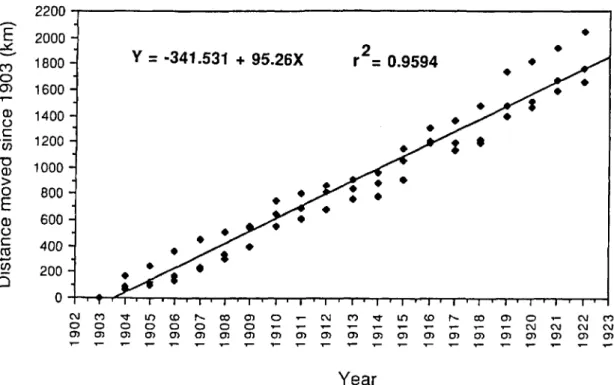
Rate of Movement. The rate of movement of the weevil infestation front was closely monitored during the early 1900s by individual cotton-pro-ducing states and the United States Department of Agriculture (USDA). Hunter & Coad (1923) pro-vided a map of the cotton belt states showing the location of the boll weevil front on an annual basis from 1892 through 1922. To determine the average annual rate of movement of this front, we estab-lished three transects approximately parallel to the Gulf of Mexico and Atlantic Coasts from the 1903 infestation front in Louisiana through the 1922 front in North Carolina (Fig. 1). These were located ap-proximately 50, 200, and 350 km from the coast. The annual distance the infestation moved from its position in 1903 along each of these transects was measured, and the relationship between dis-tance moved and time was investigated by regres-sion analysis using pooled data from the three tran-sects (PROC GLM, SAS Institute 1985b, 433-506). The Cotton Belt states east of Texas were used in developing the model because infestation fronts in Texas were such that accurate distance measure-ments could not be made on either the 200 or 350 km transects.

The relationship between the distance moved and time is almost entirely linear

(Fig.

2). The coefficient of determination (r2) from the linear

regression was 0.9594 with the slope of the regres-sion line indicating that the front advanced at a rate of 95.26

±

5.14 km (x

±

95% CL) per year. The addition of a quadratic component to the regression indicated that some curvature existed in the relationship (F

=

6.48; df

=

1, 57; P

=

0.0137). However, die quadratic component was extremely

Fig. 1. Cotton belt from Louisiana to North Carolina showing the annual infestation fronts during the initial invasion of the boll weevil (after Hunter & Goad 1923). Transects used to determine the rate of movement of the infestation are indicated asA, B,and C, at approximately50km,200km, and350 km from the coast, respectively.

small compared to the linear component (F = 1,500.27; df = 1, 57; P

<

0.0001). Addition of the quadratic term increased the coefficient of deter-mination by only 0.0041 (r2 =0.9635) so the qua-dratic component was ignored during development of the model.

Hunter & Coad (1923) indicated that the aver-age movement of the front ranged from approxi-mately 64 to 193 km/yr. In addition to this annual variation, within year variability also existed with the front moving as little as 36 km in one area and as much as 235 km in another (i.e., 1916; Fig. 1). In an attempt to explain this variation we examined movement of the infestation front in relation to available habitat and ground surface winds, the two primary factors suggested in the historical lit-erature to be responsible for determining the rate of movement (Harned 1910, Hinds 1916, Hunter

& Coad 1923).

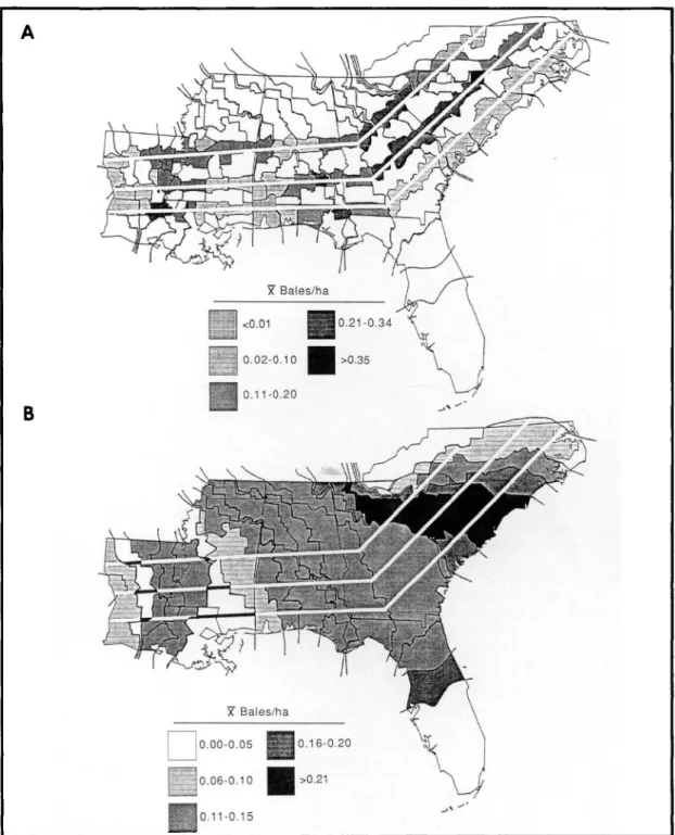
COllon Production. Harned (1910) reported that the boll weevil advanced more rapidly in areas

where cotton production was relatively low, where-as movement wwhere-as slower in arewhere-as with higher pro-duction. To examine the effect of cotton production on the movement of the infestation front during any given year, yield data (226.8 kg bale equiva-lents) were obtained for those counties having greater than half of their area falling between any two infestation fronts (Fig. 3A, B) (U.S. Depart-ment of Commerce &Labor 1906, 1907, 1908; U.S. Department of Commerce &Labor. Bureau of the Census 1909, 1910, 1911a,b; U.S. Department of Commerce. Bureau of the Census 1913, 1914; U.S. Department of Commerce. Bureau of the Census 1915-1924). Cotton yields were used as an indi-cation of the amount of cotton available to the boll weevil because the annual data on the number of hectares planted per county were not available. Because the location of annual infestation fronts was determined by the presence of boll weevils in previously uninfested areas late in the season (Hinds 1916), cotton yields for the year of infestation should

CULIN ET AL.; SIMULATION MODEL OF BOLL WEEVIL DISPERSAL April 1990

2200

-

E

2000

.x

-C'I)

1800

0 0)

₁₆₀₀

..--Q)

₁₄₀₀

u

c

1200

CJ) "0

1000

Q)

>

0

800

E

Q)

600

u

c

₄₀₀

rn

.•...

CJ)

200

0

0

y

=

-341.531 + 95.26X

_r

2

=

_0.9594

• •

•

197

•

N C') o 0 OJ OJ '<t IJ') to ,... co OJ 00000 0 OJ OJ OJ OJ OJ OJ o N OJ OJ OJ C') '<t IJ') OJ OJ OJ

Year

to ,... co .•... OJ OJ OJ OJ 0 N N OJ OJ OJ N C') N N OJ OJ

Fig. 2. Regression of distance moved by the infestation front versus time. The three data points from each year come from the transects illustrated in Fig. 1(T2 =0.9594; F =1500.27; df =1,57; P <0.0001).

not have been affected to any great extent by the arrival of the boll weevil.

Yield data were examined in two ways. First, cotton yields per hectare were calculated for all counties crossed by a transect and a Pearson prod-uct-moment correlation coefficient was computed

using the distance moved along the transect and

average yields per hectare for all counties through which the transect passed (Fig. 3A) (PROC CORR, SAS Institute 1985a, 861-874). Second, a Pearson product-moment correlation coefficient was cal-culated for the average yield for all counties having greater than half of their area between any two transects with the average movement of the infes-tation front, based on the three transects, for that year (Fig. 3B). Neither the individual transect dis-tance-county yields (Fig. 3A) (r = -0.12007, P = 0.3918, n=53), nor the averaged transect distance-area yields (Fig. 3B) (r = -0.16568, P = 0.4979, n =19) indicated a significant relationship between cotton production and distance moved by the in-festation front. These results suggest that the amount of cotton available did not influence the rate of movement of the boll weevil. For this reason, cot-ton density does not playa role in the model.

Ground Surface Winds. Hinds (1916) and Hun-ter & Coad (1923) attributed the boll weevil ad-vance across the southeastern United States to wind transport. Hinds (1916) further attributed the ex-tensive invasion of previously uninfested territory in Alabama in 1915 to SW winds generated by a

hurricane that made landfall near Galveston, Tex., on 16 August 1915. Although not reported by Hinds (1916), a second hurricane in 1915 made landfall near New Orleans, on 29 September (USDA Weather Bureau 1916, in USDA Weather Bureau 1905-1923). The relatively great advance of the

infestation in 1915 may have been caused by two

boll weevil cohorts transported on storm-generated frontal systems. In examining historical weather data, we found that for five of the seven years in which the advance of the infestation was greater than average, tropical storms were reported mak-ing landfall west of the infestation front (Table 1) (USDA Weather Bureau 1905-1923). These storms could have generated frontal systems resulting in transport of the boll weevil into previously unin-fested areas. The greatest movement of the infes-tation occurred in 1916 and was perhaps related to a tropical storm that moved over land from Mississippi to South Carolina beginning 5 July 1916 (USDA Weather Bureau 1917, in USDA Weather Bureau 1905-1923).

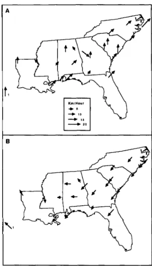
Dispersal flights of boll weevil populations occur primarily in August and September, although they have been reported to continue until frost (Hinds 1916, Hunter & Coad 1923, Taft & Jernigan 1964, Mitchell &Mistric 1965, Hopkins et al. 1971, John-son et al. 1975, Rummel et al. 1977). Data on ground surface winds are presented for August and Sep-tember 1904 through 1922 in Fig. 4A and B (USDA Weather Bureau 1905-1923). Prevailing winds were

X Bales/ha X Bales/ha <0.01 110.21-0.34 ~; :~ 0.02-0.10

II

>0.35 0.11-0.20 0.16-0.20

II

>0.21 00.00-0.05 r:=~006-0.10 0.11-0.15

B

A

Fig. 3. (A) Average cotton yields per county area for all counties crossed by each of the three transects during the initial year of boll weevil infestation. (B) Average cotton yields per county for all counties during the initial year of boll weevil infestation.

generally favorable for boll weevil dispersal into uninfested areas if emigration occurred in August, but they were generally unfavorable in September.

Boll Weevil Parameters

Population Increase. Walker (1966) and Bottrell

(1983) have reported inverse relationships between

boll weevil population density and the rate of pop-ulation increase. Bottrell (1983) indicated that low-density populations «1,235/ha) can increase 50-fold per generation, whereas at high densities (>6,175/ha) only an approximate 3-fold increase may occur. Cross (1973) reported similar figures of 2- to 40-fold increases per generation. Bottrell (1983) also reported that the percentage of larvae

surviv-April 1990 CULIN ET AL.: SIMULATION MODEL OF BOLL WEEVIL DISPERSAL 199

Table I. Reported lropical storm activity for July, Au-gust, and Spetember 1904 through 1922·

Avg.

Year advance Landfall site (date)

kmb

1904 109.4· Off Atlantic coast (14-15 Sept.) 1905 50.6 None reported

1906 60.4 Off Atlantic coast (31 Aug.) Mobile, Ala. (23-27 Sept.) 1907 84.9 North Carolina coast (1 Aug.) 1908 78.4 None reported

1909 115.9· Galveston, Tex. (21 July) Brownsville, Tex. (27 Aug.) New Orleans (21 Sept.)

1910 148.6· Florida Keys to Texas coast (6-14 Sept.) 1911 53.9 Georgia &South Carolina coast (28 Aug.) 1912 83.3 None reported

1913 45.7 None reported 1914 45.7 None reported

1915 158.4· Galveston, Tex. (16-17 Aug.) New Orleans (29 Sept.)

1916 197.6· Mississippi coast over land to South Carolina (beginning 5 July)

1917 -14.7 Mississippi &Alabama coast (22-30 Sept.) 1918 62.1 Louisiana coast (1-6 Aug.)

1919 245.~ Florida Keys to Texas (2 Sept.) 1920 62.1 Louisiana coast (21 Sept.) 1921 125.8· None reported

1922 94.8 None reported

• Data from USDA Weather Bureau (1905-1923).

bAverage distance from the three transects in Fig. 1 for each year. Asterisks indicate movement greater than the average rate of 95.26 km/yr.

ing varied from 12.5 to 0.8% for low- and high-density populations, respectively. In our model we assume a linear relationship between population density and rates of both population increase (Equation 2C) and survival (Equation 2B).

The minimum detection limit for populations in the model was set at 10 boll weevils (5 females) per hectare. This level was chosen based on an oviposition rate of approximately 300 eggs per fe-male (Lincoln 1976, Bottrell 1983), which could result in an observable number (1,500) of damaged squares per hectare.

Overwintering, Winter mortality of the boll weevil has been determined for several areas of the Southeast (Fye et al. 1959, Gaines 1959, Taft

&Hopkins 1966, Sterling 1971, Hopkins et al. 1972). Although several field-cage studies report survival rates of only 4 to 5%, Taft & Hopkins (1966) felt this to be an underestimation of actual survival. Hinds (1916), Gaines (1959), and Taft & Hopkins (1966) reported considerably greater survival rates of 40 to 45% from long-term studies under natural hibernating conditions. In addition to winter mor-tality, White & Rummell (1978) stated that only 5 to 10% of those surviving the winter successfully colonized cotton in the spring. In the model we use 40% overwintering survival with 10% of the sur-vivors successfully locating cotton in the spring.

Dispersal. We divide dispersal into three com-ponents: the proportion of the population emi-grating from a given area (block); the direction in which dispersing individuals move (toward or away

A

t,

KmfHour

.•.

_ 10

-,.

_'0 B

Fig. 4. Most commonly reported monthly average wind direction and the average speed of those winds for the period1904to1922for U.S.Weather Bureau Stations in the Southeast (A) August; (B) September. 1indicates Galveston, Tex.

from uninfested areas); and the distance (number of blocks) that they travel.

No data were located detailing what proportion of the population in a given area emigrated from that area. Following an iterative process using val-ues described below, the emigration factor in the model was set at 7.5% of the population in a block. Using an average figure of 13.2% of the total area from western Louisiana through North Carolina being planted to cotton (U.S. Census Office 1902; U.S. Department of Commerce &Labor 1913; U.S. Department of Commerce 1922, 1984) (Fig. 5A, B, C), and Hinds's (1916) estimated population densities of 12,400 to 61,800 individuals per hect-are, this would result in 930 to 4,635 emigrating boll weevils per hectare.

Although Bottrell (1983) indicated that emi-grating boll weevils move in all directions, Johnson (1969) summarizing available data on boll weevil flight stated that they are relatively weak fliers whose flight direction is primarily wind deter-mined. This is supported by flight mill data

indi-A B c

o

c::::::Jo _1'·20 c:=:J<IO _zo·z:) [:=:J10·1' _ >30

Fig. 5. The percentage of individual counties plant-ed to cotton in 1899(A), 1909 (B), 1919 (C), and 1982 (D). Boll weevil infestation fronts for 1909 and 1919 are shown on Band C, respectively.

cating that the boll weevil can not readily fly against winds over 4.8 km/h (McKibben et al. 1988). Of the 18 boll weevils collected by Glick (1939, 1957) and Glick & Noble (1961) in airplane-mounted insect nets, 67% (12) were collected at altitudes < 152.4 m. Based on these data, we assume that

dispersing boll weevils are influenced primarily by surface winds. However, a recently developed sto-chastic simulation model of boll weevil dispersal suggests that the vertical distribution of migrating individuals can have a pronounced effect on the distance an infestation could spread (McKibben & Smith 1989).

Data on the effects of surface winds on boll wee-vil dispersal have been gathered by W. A. Dick-erson & G. H. McKibben (personal communica-tion) and can be extrapolated from Johnson et al. (1975, 1976) using U.S. Department of Commerce Weather Bureau data (1971-1974, in U.S. De-partment of Commerce. Weather Bureau 1971-1980). These studies show that during August and September, 75% (Johnson et al. 1975) and 76% (Dickerson & McKibben, personal communica-tion), respectively, of marked boll weevils released and recaptured in dispersal studies moved in the direction of the prevailing ground surface winds, and 25 and 24%, respectively, moved against these winds. Johnson et al. (1975, 1976) reported no ap-parent directional component to boll weevil dis-persal in mark-release-recapture studies lasting several months when the entire recapture data set was pooled. However, this would appear to be due to considerable variation in prevailing surface wind direction during the period of their study (U.S. Department of Commerce. Weather Bureau 1971-1974, in U.S. Department of Commerce. Weather Bureau 1971-1980). In our model we allow 76% of the emigrants to move with the prevailing sur-face winds resulting in 5.7% (76% of 7.5%) of the population in a given block dispersing with the prevailing wind, while 1.8% (24% of 7.5%) move against the wind.

To incorporate a wind direction component into a linear deterministic model we made the following assumptions: (1) favorable winds, those advancing the front through the Gulf Coast states, were from the S, SW, W, and NW (180 to 315°); winds from other directions were considered unfavorable, moving boll weevils back into previously infested areas; (2) where the transects parallel the Atlantic coast, favorable winds were those from the SE, S, SW, and W (135 to 270°). For each block on each transect, the favorable to unfavorable wind ratio is based on the frequencies of the average monthly direction, for either August or September, for the closest two to four recording stations. The per-centage of time that the prevailing winds were considered to be favorable for each block is illus-trated in Fig. 6B.

Johnson et al. (1976) and W. A. Dickerson & G. H. McKibben (personal communication) have con-ducted mark-release-recapture studies during the late summer and fall migration period in which the most distant trap locations were 80.5 and 104.6 km from the release site, respectively. In both stud-ies, the majority of recaptured boll weevils moving with prevailing winds (98 and 89%, respectively) were collected in traps <48 km from the release

April 1990

A

B

CULIN ET AL.: SIMULATION MODEL OF BOLL WEEVIL DISPERSAL 201

f'ig. 6. (A) Three block transects used in the historical model. (B) Percentage of time when the prevailing ground surface winds were from directions that would transport boIl weevils in an easterly or northeasterly direction (August data above each transect; September data below each transect).

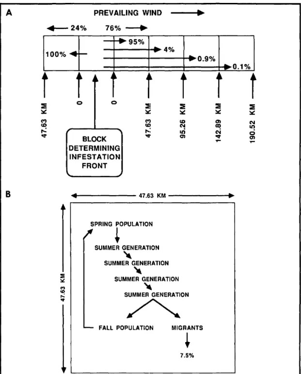
site. Using these figures as starting points, and based on the biological parameters described above, the proportion of dispersing individuals moving one, two, three, or four blocks (47.63, 95.26, 142.89, or 190.52 km) with the prevailing winds were deter-mined, through iteration, to be 95.0, 4.0, 0.9, and

0.1%, respectively (Fig. 7A). These values result in an average annual rate of movement of the infes-tation front of approximately 95.26 km. However, numbers below the minimum detection limit (

<10

individuals/ha), may occur ahead of the front. In-formation presented during the initial immigration

A

PREVAILING WIND

••

'--24%

76%

-+

~ 95%

-

4%

100% •

~

-

-0.9%

•..

_•..

0.1%

t t

~

t t t t t

~

0 0

~

~

::E

~

~

~

~

~

~

C"') C"') _co

_m

_N co

_....:

_I co

_....:

C'! IX! it! II) N 0 o:t'

BLOCK o:t'

m

o:t'

.•..

m

.•..

DETERMINING INFESTATION FRONT

B

~

47.63 KM

••

~

SPRING POPULATION

~

SUMMER GENERATION

"

SUMMER GENERATION

"

:E

_{SUMMER GENERATION}

~

M

"

CD SUMMER GENERATION

r-:

or

~

- FALL POPULATION MIGRANTS

+

7.5%

Fig. 7. (A) Model structure indicating the proportion of migrants moving with and against the prevailing winds and the proportion traveling each of the various distance steps. (B) Structure of the population growth model used to generate boll weevil densities within a given block.

of the boll weevil suggested that this situation did occur with highest populations immediately ahead of the previous infestation front and relatively low numbers determining the front for the next year

(Hinds 1916, North Carolina Agricultural Exten-sion Service 1922).

Johnson et al. (1976) and W. A. Dickerson & G. H. McKibben (personal communication), reported

April 1990 CULIN ET AL.: SIMULAnON MODEL OF BOLL WEEVIL DISPERSAL 203 4

+ ~

(MSUPOP[I, K

+

n, T] n-l .DMPERB[I, K

+

n] .MOVBn[I, K

+

n]) (4)

The non-emigrating portion of the last summer generation plus potential immigrants from the four preceding and four succeeding blocks determine the fall population (FPOP) (Equation 4).

FPOP[I, K, T]=(SUPOP[I, K, T] - MSUPOP[I, K, TJ) 4

+ ~

(MSUPOP[I, K - n, T] n-l .DMPERF[I, K - n] .MOVFn[I, K - nJ) 111,287,085 ~ SPOP[I, K, T] < 148,382,780 148,382,780 ~ SPOP[I, K, T] < 185,478,475 185,478,475 ~ SPOP[I, K, T](2B) 0.023 for 0.051 for

entering diapause within a block. Of the 7.5% that emigrate (MSUPOP), 76%(DMPERF) move with the prevailing winds and 24% (DMPERB) move against these winds. Of those moving with the pre-vailing winds 95.0% (MOVF1), 4.0% (MOVF2),

0.9% (MOVF3) and 0.1%(MOVF4) reach the next

four boxes, respectively (Eig. 7A). Of those moving against the wind 100% (MOVB1) move into the adjacent block while 0% (MOVB2, MOVB3,

MOVB4) travel farther. As with the spring

pop-ulations, fall populations do not represent gener-ations.

Directional movement is determined by assign-ing a random number between 1 and 100 to each block of the most coastal string. The same number is then assigned to corresponding blocks of the other transects (i.e., all first blocks have the same random number assigned to them, as do all second blocks, third blocks, etc.). For a given block, this number is compared with the percentage of time that fa-vorable winds were reported. If the random

num-0.008 for RINC = 50.0 for SPOP[I, K, T] < 37,095,695 44.0 for 37,095,695 ~ SPOP[I, K, T] < 74,191,390 32.5 for 74,191,390 ~ SPOP[I, K, T] < 111,287,085 20.5 for 111,287,085 ~ SPOP[I, K, TJ

<

148,382,780 9.5 for 148,382,780

s

SPOP[I, K, T] < 185,478,475 3.0 for 185,478,475

s

SPOP[I, K, T] (2C) Of the population in a block at the end of the last summer generation, 7.5% emigrate (MPER) as the migrating proportion of the summer population

(MSUPOP) (Equation 3).

MSUPOP[I, K, T] =(SUPOP[I, K, T]·MPER) (3)

SUPOP[I, K, T]=

((SPOP[I, K, T]·SUSURV)·RINC) (2A)

SUSURV = 0.125 for SPOP[I, K, T] < 37,095,695 0.110 for 37,095,695 ~ SPOP[I, K, T] < 74,191,390 0.081 for 74,191,390 ~ SPOP[I, K, T] < 111,287,085 that all boll weevils recaptured in directions op-posing the prevailing winds traveled <48 km. Based on these data, 100% of the emigrating boll weevils moving against the prevailing wind in the model move into the adjacent block.

Model Structure

The basic form of the model is illustrated in Fig. 7A & B with the variables as defined below. In developing the model, the area from western Lou-isiana through North Carolina was divided into three strings of blocks (Fig. 6A). Block size was based on the historical rate of movement of the infestation front (95.26 km/yr). This distance was then halved so that each distance step consisted of a block measuring 47.63 km by 47.63 km into, and from, which boll weevils disperse. This size ap-proximates the shortest distance the front moved based on the transect data, with the exception of negative movement reported in 1917 (Fig. 1). Like-wise, four blocks approximate the maximum dis-tance the front moved with the exception of 1916 (Fig. 1). Each block was considered to contain 30,000 ha of cotton for historical simulations (based on average 13.2% cotton cover, see above) and 3,700 ha of cotton for current conditions (based on av-erage 1.6% cotton cover; U.S. Department of Com-merce 1984).

Populations undergo four seasonal generations within each block with densities calculated as de-scribed below. In the following equations, I rep-resents the transect; K, block; and T, the year, for which population densities are being calculated.

Spring populations (SPOP) (Equation 1) deter-mine the number of individuals in a block that successfully colonize cotton in the spring.

SPOP[I, K, T] =((FPOP[I, K, T - 1]

·WINSURV)·COTLOC) (1)

It is determined by the previous fall population

(FPOP) in the block reduced by overwintering

survival (WINSURV) and the proportion of those individuals successfully locating cotton upon emer-gence (COTLOC). This population does not rep-resent a generation and so the equations do not include population growth parameters.

Each of the four summer generations (SUPOP) (Equation 2A) have a within-generation survival

(SUSURV) (Equation 2B) and rate of increase

(RINC) (Equation 2C) determined by the

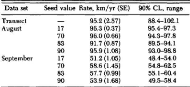
Table 2. Sensitivity analysis for MPER and seed value Table 3. Sensitivity analysis for the random number for August conditions seed value used to determine the prevailing ground surface

wind direction" Seed value MPER Rate, km/yr (SE) % Change

96.3 (0.37) Data set Seed value Rate, km/yr (SE) 90% CL, range 17 0.0750 0.0825 97.6 (0.56) +1.36 Transect 95.2 (2.57) 88.4-102.1 0.0675 92.8 (0.73) -3.61 August 17 96.3 (0.37) 95.4-97.3 70 0.0750 96.0 (0.66) 70₈₃ 96.0(0.66)_{91.7 (0.87)} 94.3-97.8_89.5-94.1 0.0825 96.9(0.60) +0.97 90 95.9 (1.08) 93.0-98.8 0.0675 92.7 (0.38) -3.44 September 17 51.2 (1.05) 48.4-54.0 83 0.0750 91.7 (0.87) 70 58.6 (1.45) 54.8-62.5 0.0825 93.3 (0.84) + 1.71 83 57.7 (0.99) 55.1-60.4 0.0675 89.5 (0.80) -2.38 90 53.9 (1.68) 49.5-58.4 90 0.0750 95.9 (1.08)

aMPER held constant at 0.075.

0.0825 96.8 (0.84) +1.02 0.0675 93.8 (0.61) -2.13

ber is less than the favorable wind percentage, for-ward migration occurs as in Fig. 7A.If it is greater than the favorable percentage, migration moves the majority of dispersing individuals back into previously infested areas.

Sensitivity Analyses. The only variable incor-porated in the model not supported by research data is the proportion of the population migrating out of any given block (MPER). In testing the sensitivity of the model to this variable, simulations were conducted using four different random num-ber seeds for the wind-driver (seed = 17, 70, 83, 90). In each of these four simulations, the MPER variable was incorporated at the base level of 7.5% and increased and decreased by 10% (8.25 and 6.75%, respectively). A 10% increase in the MPER value resulted in increases in the rate of movement, varying from 0.97 to 1.71% depending on the ran-dom number seed used. When the MPER value was decreased by 10% the predicted rate of move-ment showed a decrease ranging from -3.61 to

-2.13% (Table 2). As this variation did not ap-proach 10%, it was assumed that the model was not sensitive to slight changes in this variable.

Changes in the random number seed value did result in variations in the predicted rate of move-ment. Using the historical values for prevailing sur-face winds in August, the predicted rate of move-ment ranged from 91.76 (±0.87) to 96.35 (±0.37) km/yr; under September conditions, it ranged from 51.23 (±1.05) to 58.68 (±1.45) km/yr (MPER held constant at base value) (Table 3). Because there was overlap among the 90% confidence limits (Lit-tle &Hills 1978) among the four values for August and September (Table 3), respectively, it was de-termined that the variation due to the random number seed value chosen had a negligible effect on the predicted rates of movement. All predicted rates of movement, regardless of the seed value used, fell within the 90% confidence limit of the measured transect data (Table 3).

Current Conditions. To make the model more closely simulate current conditions, several modi-fications were made. As cotton is currently grown

in a relatively narrow belt parallel to the coast (Fig. 5D), only the two most coastal block transects are used (Fig. 8A). Prevailing ground surface wind directions and speeds for August and September were estimated using data for 1971 through 1980 (Fig. 9A and B) (U.S. Department of Commerce Weather Bureau 1971-1980). The percentage of time that these winds were favorable or unfavor-able for dispersal into the current eradication pro-gram zone is presented in Fig. 8B. A pesticide survival factor (PESTSURV) is incorporated into calculations for the spring and summer popula-tions. In the spring population pesticide mortality is induced when densities are above 360 individuals (180 females) per hectare of cotton (1,323,000 per block), while during summer generations popula-tion densities of 250 individuals (125 females) per hectare of cotton (918,800 per block) trigger pes-ticide mortality. These densities approximate thresholds of 15 (preflowering) and 10% (flowering) damaged squares with a square density of 150,000/ ha and oviposition rate of 300 eggs per female. A diapause-treatment survival factor (DIAPSURV) is incorporated into the calculation of fall population densities. Treatment thresholds for the fall popu-lations were set at two levels, one to approximate treatments based on the summer threshold (250 individuals per hectare) and the other using the presence of boll weevils (2 individuals per block) as the threshold to approximate diapause controls as they are applied within the eradication program zone.

Predictions Based on Current Conditions. Sim-ulations based on current conditions were con-ducted using a single random number seed for the wind-driver (seed =70). Mortality due to pesticide application was induced under three scenarios. First, early-, mid-, and late-season pesticide applications were triggered by population densities approxi-mating 15, 10, and 10% square or boll infestation, respectively. Second, early-, and midseason appli-cations were triggered at 15 and 10% infestation, respectively; late-season applications were trig-gered by the presence of two or more boll weevils in a block. Third, applications at any time were triggered by the presence of two or more boll

wee-April 1990

A

B

CULIN ET AL.: SIMULATION MODEL OF BOLL WEEVIL DISPERSAL

205

Fig. 8. (A) Two block transects used to predict reinfestation rates under current conditions. (B) Percentage of time when the prevailing ground surface winds were from directions that would transport boll weevils in an easterly or northeasterly direction (August data above each transect; September data below each transect).

viIs in a block. Under the current program guide-lines, if two boll weevils are trapped in or near a cotton field that field is considered to be infested and receives pesticide treatment.

Pesticide mortality also was examined at several levels. These were 0, 50, 75, or 95% mortality in

spring, summer and fall; 50% during spring and summer and 95% during fall; or 95% in spring and summer and 50% in fall.

With no induced mortality, the current condi-tions model predicts that the infestation will ad-vance into the eradication program zone at a rate

A

+,

-"

-

"

_'0

Table 5. Simulated rate of movement under current conditions when pesticide mortality is triggered by con-ventional thresholds in-season and presence in the fall"

% Mortality Rate (±SE), km/yr In-season Fall August September

0 0 74.9 (5.23) 50.2 (0.41) 50 50 57.6 (4.05) 42.7 (0.41) 75 75 42.8 (2.12) 36.2 (0.42) 95 95 11.6 (3.07) 9.7 (2.80) 50 95 19.6 (0.87) 18.2 (0.42) 95 50 54.5 (3.65) 44.9 (1.33) " Early-season 15%; midseason 10% infestation; late-season

pres-ence.

" Early-season 15%; mid- and late-season 10% infestation. Table 4. Simulated rate of movement under current conditions when pesticide mortality is triggered by con-ventional thresholds"

Fig. 9. Most commonly reported monthly average wind direction and the average speed of those winds for the period1971to1980for U.S.Weather Bureau Stations in the southeast (A) August; (B) September.

present (Tables 4 and 5). These simulations also suggested that when mortality was triggered by the high thresholds in all generations, the mortality incurred during the in-season generations had the greatest effect on determining the predicted rate of movement (Table 4), and when the mortality trigger for the fall generation was presence of boll weevils, that had the greatest effect on the pre-dicted rate of movement (Table 5). Only when induced mortality was triggered by presence in all generations was no movement predicted.

Discussion

Based on the simulation model and assumptions described here, the strategies used in the current eradication program are such that boll weevil-free areas can be maintained. However, simulations suggest that a vigilant monitoring program is nec-essary, and that any accidental infestations within boll weevil-free areas will have to be eliminated. Simulations using various mortality rates suggest that if mortality resulting from pesticide applica-tion is reduced (i.e., through resistance, changes in pesticides used, or restricted usage in some areas because of environmental concerns) the probability of maintaining weevil-free areas is greatly reduced. We feel that although this model accurately sim-ulates the historical movement of the boll weevil infestation as it moved across the southeastern United States, it could be refined through further studies on the dispersal characteristics of this species. Three areas in particular are studies concerning the proportion of migrants in local populations, long-distance mark-recapture studies (trap lines in excess of 150 km) with detailed wind data, and studies examining the altitudinal distribution of dispersing boll weevils. In a stochastic simulation model of boll weevil dispersal, McKibben &Smith (1989) have shown that the altitude of dispersing boll weevils can have a considerable effect on the distance that they travel. The back-track trajectory model of Scott & Achtemeier (1987) also has in-dicated that height of flight can affect both the distance and direction traveled by wind-borne in-sects. September 50.2 (0.41) 49.1 (0.41) 48.9 (0.54) 45.5 (1.66) 49.1 (0.41) 45.5 (1.66) Rate (±SE), km/yr August 74.9 (5.23) 70.8 (4.37) 68.0(4.19) 63.5 (4.03) 70.8 (4.35) 63.5 (4.03) Fall

o

50 75 95 95 50 % Mortality

o

50 75 95 50 95 B In-season

of 74.9 km per year if migration occurs in August or 50.2 km per year if it occurs in September (Table 4). As was expected, increasing mortality rates to 95% results in a reduction in the predicted rate of movement both when in-season and fall treatment thresholds are high and when the fall threshold is

April 1990 CULIN ET AL.: SIMULATION MODEL OF BOLL WEEVIL DISPERSAL 207

Acknowledgment

We thank Terry Pizzuto for her assistance with the tedious job of locating various pieces of historical data dealing with cotton production and weather factors, and for constructing the figures. Without her assistance this project would have been much more difficult. Suzy Mef-ferd did the artwork on Fig. 5. Peter Adler, Dave Al-verson, Bill Dickerson, Jena Johnson, Dave Parlor, Dave Smith, and perhaps others who have been inadvertently omitted, spent a considerable amount of time in discus-sions dealing with various aspects of this project. Critical reviews of earlier drafts of the manuscript by Grayson Brown, Jack Jackson, Bob Jones, Tim Mack, Gerald McKibben, Steve Roach, Mitch Roof, Mack Thomas, and one anonymous reviewer have added tremendously to its quality. The model is the result of a Special Topics Course (ENT 810) in Applied Biological Modeling of-fered by the first author. Its development was supported in part by the Office of the Dean of Resident Instruction, College of Agricultural Sciences, Clemson University. It is Technical Contribution 2785 of the South Carolina Agricultural Experiment Station, Clemson University, Clemson, S.c.

References Cited

BotlrelJ, D. G. 1976. The boll weevil as a key pest, pp. 5-8. In T. B. Davich [ed.], Boll weevil suppression, management, and elimination technology. USDA-ARS-S-71. Memphis, Tenn. (A77.15: 571).

1983. The ecological basis of boll weevil

(Anthono-mus grandis Boheman) management. Agric. Ecosys. Environ. 10: 247-274.

Cross, W. H. 1973. Biology, control and eradication of the boll weevil. Annu. Rev. Entomol. 18: 17-46. Fye, H. E., W. W. McMillian, H. L. Walker & A. L.

Hopkins. 1959. The distance into woods along a cotton field at which the boll weevil hibernates. J. Econ. Entomol. 52: 310-312.

Gaines, H. C. 1959. Ecological investigations of the boll weevil, Tallulah, Louisiana, 1915-1958. USDA-ARS, Technical Bulletin 1208. U.S. Government Printing Office, Washington, D.C. (A1.36: 1208). Glick, P. A. 1939. The distribution of insects, spiders

and mites in the air. USDA Technical Bulletin 673. U.S. Government Printing Office, Washington, D. C. (A1.36: 673).

1957. Collecting insects by airplane in Southern Tex-as. USDA Technical Bulletin 1158. U.S. Government Printing Office, Washington, D.C. (A1.36: 1158). Glick, P. A.& L. W. Noble. 1961. Airborne

move-ment of the pink bollworm and other arthropods. USDA Technical Bulletin 1255. U.S. Government Printing Office, Washington, D.C. (A1.36: 1255). Harned, H. W. 1910. Boll weevil in Mississippi, 1909.

Mississippi Agricultural Experiment Station Bulletin 139. Agricultural College, Miss.

Hinds, W. E. 1916. Boll weevil in Alabama. Alabama Agricultural Experiment Station Bulletin 188. Ala-bama Polytechnic Institute, Auburn.

Hopkins, A. H., H. M. Taft & H. R. Agee. 1971. Movement of the boll weevil into and out of a cotton field as determined by flight screens. Ann. Entomo!. Soc. Am. 64: 254-257.

Hopkins, A. L., H. M. Taft, S. H. Hoach & W. James. 1972. Movement and survival of boll weevils in several hibernation environments. J. Econ. Entomo!. 65: 82-85.

Howard, L. O. 1894. A new cotton insect in Texas. USDA, Division of Entomology. Insect Life 7: 273. Hunter, W. D.& B. H. Coad. 1923. The boll-weevil

problem. USDA, Farmers' Bulletin 1329. (A1.9: 1329). Johnson, C. G. 1969. Migration and dispersal of

in-sects by flight. Methuen, London.

Johnson, W. L., W. H. Cross, J. E. Leggett, W. L. McGovern, H. C. Mitchell &E. B. Mitchell. 1975. Dispersal of marked boll weevil: 1970-1973 studies. Ann. Entomol. Soc. Am. 68: 1018-1022.

Johnson, W. L., W. H. Cross&W. L. McGovern. 1976. Long-range dispersal of marked boll weevils in Mis-sissippi during 1974. Ann. Entomol. Soc. Am. 69: 421-422.

Lincoln, C. 1976. Seasonal development of the boll weevil.InT. B. Davich [ed.], Boll weevil suppression, management, and elimination technology. USDA-ARS-S-71. Memphis, Tenn. (A77.15: 571).

Little, T. M.&F. J. Hills. 1978. Agricultural exper-imentation. Wiley, New York.

McKibben, G. H., M. J. Grodowitz & E. J. Villavaso. 1988. Comparison of flight ability of native and two laboratory-reared strains of boll weevils (Coleoptera: Curculionidae) on a flight mill. Environ. Entomo!. 17: 852-854.

McKibben, G. H. & J. W. Smith. 1989. Weather factors affecting long-range dispersal of the boll wee-vil, pp. 250-252. In 1989 Proceedings Beltwide Cot-ton Producers Research Conference, 42nd Cotton Insects Research & Control Conference, National Cotton Council of America, Memphis, Tenn. Mitchell, E. H.& W. J. Mistric. 1965. Concepts of

population dynamics and estimation of boll weevil populations. J. Econ. Entomol. 58: 757-763. North Carolina Agricultural Extension Service. 1922.

Farming under boll weevil conditions. North Caro-lina Agricultural Extension Service of the State Col-lege & State Department of Agriculture. Extension Circular 124. Raleigh, N. C.

Hummel, D. R., L. B. Jordan, J. R. White & L. J. Wade. 1977. Seasonal variation on the height of boll weevil flight. Environ. Entomo!. 6: 674-678.

SAS Institute. 1985a. SAS user's guide: basics, version 5 Ed. SAS Institute, Cary, N. C.

1985b. SAS user's guide: statistics, version 5 Ed. SAS Institute, Cary, N. C.

Scott, H. W. &G. L. Achtemeier. 1987. Estimating pathways of migrating insects carried in atmospheric winds. Environ. Entomo!. 16: 1244-1254.

Sterling, W. L. 1971. Winter survival of the boll wee-vil in the high and rolling plains of Texas. J. Econ. Entomal. 64: 39-41.

Taft, H. M.&A. H. Hopkins. 1966. Effect of different hibernation environments on survival and movement of the boll weevil. J. Econ. Entomol. 59: 277-279. Taft, H. M. & C. E. Jernigan. 1964. Elevated screens

for collecting boll weevils flying between hibernation sites and cottonfields. J. Econ. Entomo!. 57: 773-775. U.S. Census Office. 1902. Twelfth census of the United States, taken in the year 1900. Agriculture Part II, Crops &Irrigation. U.S. Government Printing Office, Washington, D.C. (C3.900/5: 6/pt.2).

USDA-APHIS. 1986. The stamper: boll weevil erad-ication news, Vol. 4, No.7, Oct 21, 1986.

USDA Weather Bureau. 1905-1923. Report of the chief of the weather bureau 1904-1905-1921-1922. U.S. Government Printing Office, Washington, D.C. (C30.1: 1905-1923).

census of the United States, taken in the year 1920. Vol. VI, part 2, Agriculture. U.S. Government Print-ing Office, WashPrint-ington, D.C. (C3.28/5: 6/pt.2). 1984. 1982 Census of agriculture. Vo\. 1. Geographic

area series. State and county data. U.S. Government Printing Office, Washington, D.C. (C3.31/4: 982). U.S. Department of Commerce. Bureau of the Census.

1913, 1914. Cotton production 1912& 1913. U.S. Government Printing Office, Washington, D.C. (C3.3: 116& C3.3: 125).

1915-1924. Cotton production and distribution, sea-son of 1914-1915-1922-1923. U.S. Government Printing Office, Washington, D. C. (C3.3: 131, C3.3: 134, C3.3: 135, C3.3: 140, C3.3: 145, C3.3: 147, C3.3: 150, C3.3: 153).

U.S. Department of Commerce. Weather Bureau. 1971-1980. Climatological data. National Sum-mary. U.S. Government Printing Office, Washington, D.C. (C55.214: 22-31).

U.S. Department of Commerce and Labor. 1906. Cotton production and statistics of cottonseed prod-ucts: 1905. U.S. Government Printing Office, Wash-ington, D. C. (C3.3: 40).

1907,1908. Cotton production 1906, 1907. U.S. Gov-ernment Printing Office, Washington, D.C. (C3.3: 76 & C3.3: 95).

1913. Thirteenth census of the United States, taken in the year 1910. Vo\. VI. Agriculture 1909& 1910. U.S. Government Printing Office, Washington, D.C. (C3.16: 6).

U.S. Department of Commerce and Labor. Bureau of the Census. 1909, 1910, 1911a. Cotton produc-tion 1908, 1909, 1911. U.S. Government Printing Of-fice, Washington, D.C. (C3.3: 100, C3.3: 107, C3.3: 114).

1911b. Cotton production and statistics of cottonseed products: 1910. U.S. Government Printing Office, Washington, D.C. (C3.3: 111).

Walker, J. K. 1966. The relationship of the fruiting of the cotton plant and over-wintered boll weevils to the F, generation.

J.

Econ. Entomo\. 59: 323-326. White, J. R. & D. R. Rummel. 1978. Emergence

profile of overwintered boll weevils and entry into cotton. Environ. Entomo\. 7: 7-14.