HAL Id: hal-00727353
https://hal-upec-upem.archives-ouvertes.fr/hal-00727353
Submitted on 26 Feb 2018
HAL is a multi-disciplinary open access
archive for the deposit and dissemination of
sci-entific research documents, whether they are
pub-lished or not. The documents may come from
teaching and research institutions in France or
abroad, or from public or private research centers.
L’archive ouverte pluridisciplinaire HAL, est
destinée au dépôt et à la diffusion de documents
scientifiques de niveau recherche, publiés ou non,
émanant des établissements d’enseignement et de
recherche français ou étrangers, des laboratoires
publics ou privés.
Topology on digital label images
Loïc Mazo, Nicolas Passat, Michel Couprie, Christian Ronse
To cite this version:
Loïc Mazo, Nicolas Passat, Michel Couprie, Christian Ronse. Topology on digital label images. Journal
of Mathematical Imaging and Vision, Springer Verlag, 2012, 44 (3), pp.254-281.
�10.1007/s10851-011-0325-8�. �hal-00727353�
Journal of Mathematical Imaging and Vision
Topology on digital label images
--Manuscript
Draft--Manuscript Number: JMIV-806R2
Full Title: Topology on digital label images
Article Type: Manuscript
Keywords: digital imaging; topology; label images; homotopy; simple points. Corresponding Author: Loïc Mazo
Illkirch, FRANCE Corresponding Author Secondary
Information:
Corresponding Author's Institution: Corresponding Author's Secondary Institution:
First Author: Loïc Mazo
First Author Secondary Information:
All Authors: Loïc Mazo
Nicolas Passat Michel Couprie Christian Ronse All Authors Secondary Information:
Topology on digital label images
JMIV-806
Answers to Editor / Reviewers
Lo¨ıc Mazo, Nicolas Passat, Michel Couprie, Christian Ronse
December 19, 2011
Response to the Editor:
Editor: We have received the reports from our advisors on your manuscript, ”Topology on digital label images”, which you submitted to Journal of Mathe-matical Imaging and Vision.
Based on the advice received, the Editor feels that your manuscript could be accepted for publication should you be prepared to incorporate minor revisions. When preparing your revised manuscript, you are asked to carefully consider the reviewer comments, which are attached, and submit a list of responses to the comments. Your list of responses should be uploaded as a file in addition to your revised manuscript.
Authors: We would like to thank the Editor for the management of the
re-view process of this manuscript. It has been revised by taking into account the suggestions of the reviewer.
Response to Reviewer
#2:
Authors: We would like to thank the Reviewer for having taken time to evaluate
our manuscript. A point-by-point response to each of the issues raised by the Reviewer is given below.
Referee: The authors have made different corrections that significantly improve their article. However, I would greatly appreciate that some efforts will be made to give an easier access to the paper content for novice readers.
For example, add some references at the beginning of section 2.1, the books of Munkres (Elements of Algebraic Topology), Hatcher (Algebraic Topology) or Giblin (Graphs, Surfaces and Homology) are valuable references for novice reader. When adding references pay particular attention to the availability of it and be sure that the style and the way of the concepts are presented are adapted to the ”modern” readers. For example, page 4 line 36: of course Whitehead as defined elementary transformations on complexes but I am not that this reference is easy to find and it would really help the reader, again a book like Giblin’s book is more adapted.
Authors: We have added these references together with Maunder (Algebraic
Topology) and May (A Concise Course in Algebraic Topology).
Page 4 line 36: we have given two references, the original one (which is freely available on the web) and Giblin’s book.
Referee: Page 4, line 9, second column: You talk about topological spaces with base points without introducing them. After lines 12 and following: The tentative explanation about weak homotopy equivalence is very hard to follow if you don’t know what is the homotopy class of a map.
Authors: A subsection about homotopy have been added in order to introduce
the minimal knowledge of algebraic topology that is needed in the paper.
Referee: page 5 line 2: exemple 24 is very far from this text.
Authors: A new figure has been added just after the text.
Referee: page 5 section 2.3: in the first paragraphe you talk about A-space and the about Alexandroff space this is puzzling.
Authors: This has been corrected.
Referee: page 6, lines 45-50. You use property 3 that is given below and you refer to property 6 that is on page 6 in section 2.4 after the introduction of unipolar points. Please reconsider the redaction of this paragraph.
Authors: The paragraph has been rewritten (and the references to properties 3
Journal of Mathematical Imaging and Vision manuscript No. (will be inserted by the editor)
Topology on digital label images
Lo¨ıc Mazo · Nicolas Passat · Michel Couprie · Christian Ronse
Received: date / Accepted: date
Abstract In digital imaging, after several decades devoted to the study of topological properties of binary images, there is an increasing need of new methods enabling to take into (topological) consideration n-ary images (also called label images). Indeed, while binary images enable to handle one object of interest, label images authorise to simultaneously deal with a plurality of objects, which is a frequent require-ment in several application fields. In this context, one of the main purposes is to propose topology-preserving transfor-mation procedures for such label images, thus extending the ones (e.g., growing, reduction, skeletonisation) existing for binary images. In this article, we propose, for a wide range of digital images, a new approach that permits to locally modify a label image, while preserving not only the topol-ogy of each label set, but also the topoltopol-ogy of any arrange-ment of the labels understood as the topology of any union of label sets. This approach enables in particular to unify and extend some previous attempts devoted to the same purpose.
Keywords digital imaging · topology · label images · homotopy · simple points
The research leading to these results has received funding from the French Agence Nationale de la Recherche (Grant Agreement ANR-2010-BLAN-0205).
Lo¨ıc Mazo, Nicolas Passat, Christian Ronse
Universit´e de Strasbourg, LSIIT, UMR CNRS 7005, France Tel.: +33-368854413
Fax: +33-368854455 E-mail: [email protected] Lo¨ıc Mazo, Michel Couprie
Universit´e Paris-Est, Laboratoire d’Informatique Gaspard-Monge, ´
Equipe A3SI, ESIEE Paris, France
1 Introduction
In a digital image, when performing processes such as reg-istration, deformation or thinning, the preservation of the topological properties of the objects contained in the image (e.g., connected components, tunnels, cavities, etc.) is an im-portant requirement. For 50 years, several tools enabling the analysis (adjacency graphs, digital fundamental groups, ho-mology groups –see, e.g., [1, 2, 3]) and the modification un-der topological constraints (simple points, P-simple points, simple sets –see, e.g., [4, 5, 6, 7]) of binary images have been proposed and used. Nevertheless, in many fields (e.g., med-ical imaging, remote sensing, computer vision), an image is generally composed of several objects, and it is often impor-tant to understand or maintain their topological properties all together, that is the topology of each and the topology of the scene. In such images, the objects are characterised by specific labels on which there generally exists no meaning-ful order relation (unlike grey-level images for instance).
1.1 Previous works
To the best of our knowledge, the literature about topology in label images is quite limited and generally motivated by practical considerations. The most common approach is to consider only one label at a time, the other labels being mo-mentarily considered as a part of the background. However, except in the most simple cases where the label configura-tion leads to a binary modelling (see, e.g., [8, 9]), one cannot directly deal with the relations between the labels but only with the topology of each label and of its associated back-ground [10, 11, 12] (if necessary, one uses in addition an ad-jacency tree between labels in order to control their topo-logical relations). These methods are often used with a cost function, which depends on the applicative context, whose
*Manuscript
Click here to download Manuscript: gestionLabels_en_href.tex Click here to view linked References
1 2 3 4 5 6 7 8 9 10 11 12 13 14 15 16 17 18 19 20 21 22 23 24 25 26 27 28 29 30 31 32 33 34 35 36 37 38 39 40 41 42 43 44 45 46 47 48 49 50 51 52 53 54 55 56 57 58 59 60 61
Fig. 1 An image with two labels (in grey and black). If we consider
the grey label as the object of the picture using the (8,4)-adjacency pair (8-adjacency for the object and 4-adjacency for the background), the object is a ring. The black pixels together then form the inner nent of the background, while the white pixels form the outer compo-nent. However, if we now consider the black pixels as the object (still in 8-adjacency), rejecting grey pixels to the background, these latters must be understood with the 4-adjacency and they appear to have two connected components, one inside the black torus and one outside.
purpose is to assign a given label, or not, to a point of the image. Thereby points go from background to a label or vice
versa but not from a label to another. Note that some points
may sometimes take an undetermined status since they can-not be assigned a label without breaking a topology defined by an a priori knowledge or to avoid object crossings when the objects are seen under the filter of the 8-adjacency in the plane or 26-adjacency in the space (see Figure 1). The question of the adjacencies to be used in a digital label im-age is a recurrent issue. Indeed, in digital topology, in the framework developed by Rosenfeld [13], the object and the background of an image are understood with different (dual) adjacencies [14]. So, when objects in a label image are pro-cessed one at a time, being alternately the object and part of the background, they are inevitably seen under two distinct
adjacencies1. For instance, an object can have one connected
component at one step of the process and two components at the next step though no change did occur on the image (see Figure 1).
To overcome this problem, a class of “well composed” images has been defined in which the same adjacency re-lation can be used for the object and the background. This adjacency relation is necessarily the 4-adjacency in 2D im-ages and the 6-adjacency in 3D imim-ages [17]. This class of images is obtained by excluding all the images in which at least one of the three configurations depicted on Figure 2 ap-pears. In other words, it is assumed in these images that the boundaries of the objects (viewed as an union of n-cubes) are (n − 1)-manifolds. In the case where label images present forbidden configurations, an algorithm has been proposed to
1 This problem is sometimes disregarded. For instance, in [15]
(proof of Proposition 2), it is claimed “Since the 18-neighbourhood of x is limited to binary case, and by definition of simple points the topology of the complementary of R is preserved: we can deduce that the topology of X [the complementary of R in the 18-neighbourhood of
x] is also preserved, and thus that x is simple for X”. It is not clear here
what is meant by preserving topology. However, in the framework of simple points [16], it is not true in general that we can swap the object and the background without swapping together the adjacency pair.
(a) (b) (c)
Fig. 2 Forbidden configurations in (binary) well composed images.
(a) In Z2. (b,c) In Z3(configuration (b) shall not appear neither in the
object nor in the background). A label image is well composed if each binary image obtained by isolating a particular label is well composed.
dispose of them [18]. However, since the objects identified by the labels are sequentially “repaired”, one needs first to determine an order on the labels, and this order biases the result.
Another approach [19] takes further the specificity of la-bel images into account. A notion of “homotopy set” is de-fined, which is the set of the labels that can be assigned to a point without modification on the topology of each label and of its complement in the image. A local criterion is provided to decide whether a particular label belongs to the homotopy set of a point or not. Thereby, a point can move from a label to another and not solely from the background to a label or
vice versa.
In [20], the authors go further and require, before any change of label at a point, the guarantee that not only the topology of each label will be preserved but also the topol-ogy of the unions of two labels in 2D images and of three la-bels in 3D images (see Figure 3). Nevertheless, this request is not sufficient. Figure 3(c) provides a counterexample in 2D where there is the need to consider the union of three labels.
In [15], the authors study 3D label images with a frontier approach. The 3D image is divided into regions which are 6-connected (hence, the configurations of Figure 2 cannot oc-cur) and in which the voxels share the same label. Moreover, they only take into account the 6-adjacency between regions. To move a voxel x from a region A to another region B, the authors make requirements on surfaces between x and A\{x} (resp. between x and B \ {x}): they have to be homeomorphic to a 2-disk. Furthermore, for each region C 6-adjacent to x, the frontier between the regions A and C before the move
(resp. between B and C after the move), must collapse2onto
the corresponding frontier after the move (resp. before the move).
2 Here, collapse is the classical operation on complexes defined by
Whitehead [21] (see Section 2.2). 1 2 3 4 5 6 7 8 9 10 11 12 13 14 15 16 17 18 19 20 21 22 23 24 25 26 27 28 29 30 31 32 33 34 35 36 37 38 39 40 41 42 43 44 45 46 47 48 49 50 51 52 53 54 55 56 57 58 59 60
2 2 2 3 1 4 2 1 1 1 (a) 2 2 2 3 4 4 2 1 1 1 (b) 2 4 4 1 3 3 1 3 3 (c)
Fig. 3 (a) An image with four labels. (b) The label of a single pixel has
changed. Neither the topologies of the labels nor of their complements in the image are modified. However, the topology of the partition is not preserved in the sense that the union 1 + 2 becomes contractible, 1 + 3 is split into two components in 4-adjacency, 3 + 4 loses a component, 2 + 3 + 4 loses a component in 4-adjacency. (c) This example is from [20]. The authors observe that, if we look at the picture with the (8, 4)-adjacency pair, the central pixel can move from 3 to 2 without altering the topologies of the four labels and of the six pairs of labels but they do not take into consideration the union 1 + 3 + 4 though it passes from a ball to a ring. Observe also that the well-composedness of this image is destroyed by the move of the central pixel from 3 to 2.
1.2 Purpose
The aim of this article is to study the topology of label im-ages, following the idea to preserve any union of labels, which amounts to require topologically sound procedures on digital label images not to change the topological char-acteristics of the sets of a partition of Znand of any coarser
partition of the initial one. In other words, one could say that the actual set of objects in a digital label image is the power set of the partition. We have adopted a theoretical stand-point with the will to cover a wide range of situations. In our framework, we do not make any assumption on the topolo-gies of individual objects (we do not use a priori knowl-edge) and there is no forbidden configurations. Weak ho-motopy equivalence in finite spaces (which corresponds to homotopy equivalence in continuous ones) is used to per-form topological comparisons. To avoid the pitfall of dis-tinct adjacency pairs on the same object described above, we embed the digital space of the image into a richer space equipped with a genuine topology, that is a poset whose min-imal points are the points of the digital image. This enrich-ment of the space leads us to embed also the label set into a richer one, namely an atomistic lattice whose atoms are the labels of the digital image. Thereby, we can extend the digital image on its poset, assigning extended labels to new points, and we can define gradual modifications of the im-ages more adapted to topology preservation.
1.3 Contribution and structure of the article
The remainder of this article is organised as follows. Section 2 gathers results on binary images on which re-lies our work. It is intended to make the article self-contained and to introduce our notations. The last subsection of
Sec-tion 2 establishes, in particular, two new results whose proofs are provided in Appendix B and C.
In Section 3, we introduce our framework for the topo-logical understanding of label images. We describe a first tool to locally modify such a label image while keeping un-changed all homotopy groups of the objects and their unions (to be more precise, we have weak homotopy equivalences).
When the poset is the space Fnof cubical complexes defined
in Section 2, our tool keeps also unchanged the homotopy groups of the complements. Furthermore, the changes can be processed in parallel under certain conditions, thus lead-ing to well-balanced algorithms.
In Section 4, we are interested in images in which the sets of points that share a label (we say the support of the la-bel) are closed sets, as in (26, 6) digital images. In this case, we define an elementary modification, named cut, inspired by collapses. It has the same (good) topological properties as the one defined in Section 3 while the supports of the labels remain closed sets.
In Section 5, we study regular images in which the label of a point in the poset is defined by the labels of the minimal points beneath it. Regular images can be built from
digi-tal images defined on Zn and we have proved in [22] that,
when the poset is the space of cubical complexes, this con-struction puts in one-to-one correspondence the connected components of the regular image with the ones of the dig-ital image. Moreover, it induces isomorphisms between the fundamental groups of the regular image and the digital fun-damental groups of the digital image (as defined in [2]). In regular images, we give conditions for cuts to preserve regu-larity allowing thereby to modify a regular image in a topo-logically sound manner, the result being also a regular image (allowing to go back to Zn).
Section 6 concludes this paper and describes further works in preparation.
2 Simplicity in sets
The aim of this section is to gather notions and results on which relies this work, and also to present our notations. Note that in Section 2.8, we establish (new) results which are specific to complexes. Operations and relations on functions (in particular, on images) will always be implicitly pointwise ones.
2.1 Homotopy
Two continuous maps f , g : X → Y are homotopic if there exists a continuous map, called a homotopy, h : X × [0, 1] →
Y such that h(x, 0) = f (x) and h(x, 1) = g(x) for all x ∈ X.
The spaces X and Y are homotopy equivalent (or have the same homotopy type) if there exist two continuous maps
1 2 3 4 5 6 7 8 9 10 11 12 13 14 15 16 17 18 19 20 21 22 23 24 25 26 27 28 29 30 31 32 33 34 35 36 37 38 39 40 41 42 43 44 45 46 47 48 49 50 51 52 53 54 55 56 57 58 59 60 61
f : X → Y and g : Y → X, called homotopy equivalences,
such that g ◦ f is homotopic to the identity map idXand f ◦ g
is homotopic to idY. If X and Y are homeomorphic, they are
homotopy equivalent: given a homeomorphism ϕ between
X and Y, ϕ and ϕ−1are homotopy equivalences between X and Y. The converse is not true in general (for example, a ball is homotopy equivalent –but not homeomorphic– to a point). A topological space is contractible if it has the ho-motopy type of a single point. Let X be a topological space. Two paths p, q in X are equivalent if they have the same extremities (i.e., p(0) = q(0) and p(1) = q(1)) and are ho-motopic by an homotopy h such that h(0, u) = p(0) = q(0) and h(1, u) = p(1) = q(1) for all u ∈ [0, 1]. It is easy to check that this relation on paths is actually an equivalence relation. We write [p] for the equivalence class of p. If p, q are two paths in X such that p(1) = q(0) we can define the product p · q by:
(p · q)(t) =( p(2t) if t ∈ [0,
1 2], q(2t − 1) if t ∈ [12,1].
This product is well defined on equivalence classes by [p] · [q] = [p · q]. Let x be a point of X. A loop at x is a path in X which starts and ends at x. The product of two loops at x is a loop at x and the set π1(X, x) of equivalence classes of loops
at x is a group for this product. It is called the fundamental
group of X (with basepoint x) or the first homotopy group of X. If X is path-connected, the group π1(X, x) does not depend
on the basepoint (i.e., for any points x, y ∈ X, π1(X, x) and
π1(X, y) are isomorphic). Higher homotopy groups, denoted
πn(X, x), are defined by replacing loops at x by continuous
maps from [0, 1]n to X that associate the boundary of the
n-cube to x. The product on such maps is then defined by
gluing two faces of the n-cubes:
p · q(t1, . . . ,tn) =
( p(2t1,t2, . . . ,tn) if t1 ∈ [0,12], q(2t1− 1, t2, . . . ,tn) if t1 ∈ [12,1].
Conventionally, the set of path-connected components of X is denoted by π0(X, x), but it has no group structure.
A continuous map f : X → Y is a weak homotopy
equiv-alence if the morphisms fn : πn(X, x) → πn(Y, y) defined by fn([p]) = [ f ◦ p] are all bijective ( f0is just a bijection, not
a morphism). Two spaces X, Y are weakly homotopy
equiva-lent if there is a sequence of spaces X0 = X, X1, . . . ,Xr = Y (r > 1) such that there exist weak homotopy
equiva-lences Xi−1 → Xi or Xi → Xi−1 for all i ∈ [1, r]. Two
ho-motopy equivalent spaces are weakly hoho-motopy equivalent. The converse is not true in general but Whitehead’s theorem [28] implies that it is true for all spaces that are geometric realisations of simplicial or cubical complexes.
Two weakly homotopy equivalent spaces X, Y have iso-morphic homotopy groups. However, a weak homotopy equi-valence is much more than a collection of isomorphisms between homotopy groups. On Figure 4, we have depicted
two cubical 3-complexes X and Y such that Y ⊂ X. Their geometric realisations have the same homotopy type and, therefore, are weakly homotopy equivalent. Nevertheless, it is clear that the inclusion i : Y → X is not a weak homo-topy equivalence for it associates non-contractible loops to contractible loops. Likely, in image processing, we would reject such a thinning. So, the nature of the weak homotopy equivalence is an important information.
(a) (b)
Fig. 4 (From [29]) (a) A cubical 3-complex X. (b) A subcomplex Y.
Their geometric realisations have the same homotopy type. However, the inclusion i : Y → X is not a weak homotopy equivalence.
There is a case in which the weak homotopy equivalence reduces to the knowledge of the homotopy groups. When a set is weakly homotopy equivalent to a point, then it is con-nected and all its homotopy groups are trivial. Thus, obvi-ously, any constant map is a weak homotopy equivalence. Such a space is said to be homotopically trivial. There are spaces that are homotopically trivial and that are not con-tractible as shown on Figure 5.
Fig. 5 A set of points (in red), closed lines (in yellow) and closed
squares (in green) of R3whose union forms a hollow cube with a fence.
Equipped with the inclusion, this set is a finite topological space (see below Subsection 2.4) that is homotopically trivial but not contractible (the reader will be able to establish the proofs of these two assertions after the reading of Subsections 2.5 and 2.6).
2.2 Complexes
We do not recall definitions about simplicial complexes which are generally well known. The reader who whishes to rec-ollect such a notion, or any one rapidly exposed below, is invited to find complementary information in a lecture book on algebraic topology, e.g. [30, 31, 32, 33, 34]. In digital ages, grids are often cubic ones. It is then convenient, in im-age analysis, to replace simplices in complexes by n-cubes.
1 2 3 4 5 6 7 8 9 10 11 12 13 14 15 16 17 18 19 20 21 22 23 24 25 26 27 28 29 30 31 32 33 34 35 36 37 38 39 40 41 42 43 44 45 46 47 48 49 50 51 52 53 54 55 56 57 58 59 60
As cubical complexes are not commonly used, we recall hereafter the main basic definitions (see also [23]). We set
F10 = {{a} | a ∈ Z} and F1
1 = {{a, a + 1} | a ∈ Z}. A subset f of Znwhich is the Cartesian product of m elements of F1 1
and n − m elements of F10is a face or an m-face (of Zn), m is the dimension of f , and we write dim( f ) = m. We denote by Fn
mthe set composed of all m-faces of Zn and by Fnthe
set composed of all faces of Zn. Let f ∈ Fn be a face. The
set {g ∈ Fn | g ⊆ f } is a cell and any union of cells is an
abstract cubical complex. The geometric cubical complexes
are defined in the same manner, except that we change the definition of F11by setting F11={[a, a + 1] | a ∈ Z} ⊂ Rn. The
geometric realisation |K| of a geometric cubical complex K is the union of its faces. Figure 6 illustrates these definitions.
b d a c (a)
1
(b)Fig. 6 (a) Four points in Z2, a = (i, j), b = (i + 1, j), c = (i + 1, j + 1),
d = (i, j + 1). The faces f = {a}, g = {b, c} = {i + 1} × { j, j + 1} and h = {a, b, c, d} = {i, i + 1} × { j, j + 1} are symbolically depicted with
ellipses. (b) Another (more semantic) symbolic representation, often used in this article. In black, the 0-face f . In dark grey, the 1-face g. In light grey, the 2-face h.
Whitehead [21] (an easier reference for modern read-ers is [34]) has defined elementary transformations on com-plexes as follows. Let X be a complex (simplicial or cubical) and (x, y) a pair of faces in X such that x is the only face of
X including y (i.e., X \ {x, y} is still a complex). Then, (x, y)
is a free pair, and the set Y = X \ {x, y} is an elementary
collapse of X, or X is an elementary expansion of Y. If a set Y is obtained from X by a sequence of elementary collapses
(a sequence of elementary collapses and expansions), then Y is a collapse of X (X and Y are simple-homotopy equivalent or X and Y have the same simple-homotopy type) and one write X ց Y (X ցY). A set is collapsible if it collapses onto a singleton.
If Y is a collapse of X then |Y| is a strong deformation re-tract of |X| and thus |X| and |Y| are homotopy equivalent [21]. Figure 7 illustrates this property. In particular, if the complex is collapsible, its geometric realisation is contractible. The converse is not true as shown by the thin version of Bing’s house with two rooms [26] or by Zeeman’s dunce hat [27].
Fig. 7 (a) A complex X. (d) A complex Y which is an elementary
collapse of X. (b-c) Two steps in a strong deformation retraction of |X| onto |Y|.
2.3 Partially ordered sets
The motivation for considering partially ordered sets (or
po-sets) comes from (i) the observation that digital images are
essentially finite (even when they are defined on Znto avoid
difficulties on boundaries), (ii) that finite topological spaces of interest have the T0-separation property3but not the T1
-separation property4(otherwise either some points could not
be distinguished from a topological viewpoint or the space is totally disconnected), and (iii) that T0-spaces in which any
intersection of open sets is an open set (as in finite spaces) are posets [35, 36] (this point is developed in Section 2.4).
Let X be a set. A binary relation on X is a partial order if it is reflexive, antisymmetric, and transitive. A partially
ordered set, or poset, is a couple (X, ≤) where the relation ≤
is a partial order on X. The relation ≥, defined on X by x≥y iff y≤x, is a partial order on X called the dual order. We say that two points x, y in X are comparable if x≤y or y≤x. If, for all pairs (x, y) of elements of X, x and y are comparable, the relation ≤ is a total order on X. We write x < y when
x≤y and x , y and we set:
– x↑={y ∈ X | x≤y} and x↑⋆= x↑\ {x} = {y ∈ X | x < y};
– x↓={y ∈ X | y≤x} and x↓⋆= x↓\ {x} = {y ∈ X | y < x}.
If x and y are comparable, we write x ≍ y; otherwise, we write x - y. The set of points comparable with a given point
x is denoted xl (xl = x↓∪ x↑), and we set xl⋆ = xl\ {x} =
x↓⋆∪ x↑⋆. A point x ∈ X is minimal if x↓={x} and maximal
if x↑={x}. A point x ∈ X is the minimum of X if x↑= X and
is the maximum of X if x↓= X. We say that a poset is locally
finite if for each point x in X, there are finitely many points
comparable with x. A chain in X is a totally ordered subset of X. The length of a chain is its cardinality minus one. The
length of a poset X is the maximal length of a chain in X
if such a maximum exists5. The height of a point x ∈ X,
denoted ht(x), is the length of x↓. If x < y and there is no
3 A space has the T
0-separation property if for any pair of distinct
points there exists an open set that contains one of them and not the other.
4 A space has the T
1-separation property if for any ordered pair of
distinct points there exists an open set that contains the first of them and not the other. Now, let x be a point in a finite T1-space X. For
each y ∈ X, y , x, there exists an open neighbourhood of x, Uy, not
containing y. Hence, {x} =T Uyis open, that is to say, the topology on
X is the discrete topology in which all subsets are both open and closed
and the only connected sets are the singletons.
5 Some authors define the length of a chain as its cardinality and the
the maximal length of a chain in X is also called the height of X. 1 2 3 4 5 6 7 8 9 10 11 12 13 14 15 16 17 18 19 20 21 22 23 24 25 26 27 28 29 30 31 32 33 34 35 36 37 38 39 40 41 42 43 44 45 46 47 48 49 50 51 52 53 54 55 56 57 58 59 60 61
e (3)
d (2)
c (1)
b (1)
a (0)
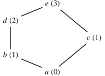
Fig. 8 The Hasse diagram of a poset defined by the set
{a, b, c, d, e} equipped with the order {(a, a), (a, b), (a, c), (a, d), (a, e),
(b, b), (b, d), (b, e), (c, c), (c, e), (d, d), (d, e), (e, e)}. Between parenthe-ses, we give the height of the points. The length of this poset is 3.
z such that x < z < y, we say that y covers x and we write x ≺ y. The Hasse diagram of the relation ≤ is the oriented
graph of the relation ≺. When orienting all arcs from bottom to top, this diagram offers a good visual representation of (small) posets (see Figure 8).
Simplicial or cubical complexes equipped with the in-clusion, ⊆, or its dual, ⊇, are locally finite posets. Moreover, for all n ∈ N, (Fn, ⊇) is order isomorphic to (Fn, ⊆) (that is,
the combinatorial properties of the k-faces of Fnare equal to
the ones of the (n − k)-faces if we replace ⊆ by ⊇). Note that it is not true for simplicial complexes.
We extend to posets Whitehead’s definitions of free pairs and collapses. A pair (x, y) in a poset X is a (combinatorial)
free pair if x is the only point (strictly) less than y in X. If
(x, y) is a free pair in X, the set X \ {x, y} is a collapse of X. When we can “thin” a subset Y of X to a subset Z of X by withdrawal of free pairs, we write Y ց Z.
2.4 A-spaces
A topological space X is an A-space if any intersection of open sets is an open set. In such a space, closed sets sat-isfy the definition properties of open sets (∅, X are closed sets, any union and any intersection of closed sets is a closed set), so one can exchange open and closed sets. The obtained topology is then called the dual topology. As any set has a closure, any element x of an A-space has a smallest
neigh-bourhood (an open set included in any open set containing x), denoted by Ux, which is the closure of {x} for the dual
topology. Conversely, a topological space X in which each point has a smallest neighbourhood is an A-space.
A T0 A-space is an A-space that has the T0-separation
property (i.e., for any two distinct points x, y, there exists a neighbourhood containing just one of them). McCord has proved in [37] that if an A-space is not T0, the identification
of the points that share the same smallest neighbourhood
leads to a homotopy equivalent quotient space which is T0.
There exists a canonical link between T0A-spaces and
posets, established by Alexandroff.
Theorem 1 ([35]) Let X be an T0 A-space. The relation ≤
defined on X by x≤y if x ∈ Uy is a partial order on X. Conversely, let (X, ≤) be a poset. The set U defined by U =
{U ⊆ X | ∀x ∈ U, x↓ ⊆ U} is a topology on X, the poset
X equipped with this topology is an T0A-space and, for all x ∈ X, Ux= x↓.
Indeed, the choice to set x≤y if x ∈ Uyis purely arbitrary.
We could set x≤y if y ∈ Uxand in literature both settings can
be found (for instance, the choice x≤y if y ∈ Uxis made by
[35, 38] and the other choice by [37, 39, 40, 41]).
If Y is a subset of X, the topology associated to the poset (Y, ≤) is the topology induced by the one associated to the poset (X, ≤). The dual topology of the topology associated to the poset (X, ≤) is the topology associated to the dual order
≥.
From now on, posets will always be equipped with the topology U described in Theorem 1. This topology leads to a nice characterisation of continuous maps.
Property 2 ([39]) Let X, Y be posets. A function f : X → Y
is continuous iff it is non-decreasing.
In the sequel, we will often have to test if a poset is con-tractible. Remember that a space is contractible if it has the homotopy type of a point, that is, if there exists a continu-ous map H : X × [0, 1] → X such that H(x, 0) = x for any
x ∈ X and x 7→ H(x, 1) is a constant map. Intuitively, a set is
contractible if it can be continuously shrunk to a point. Nev-ertheless, this intuition is of little help in a finite space. For instance, consider a geometric cubical complex X composed of a closed unit square of R2, together with all its faces. Say, it is the one depicted on Figure 9(a). This complex is col-lapsible by X ց X \ {a, b} ց {d, e, f , h, i} ց {e, f , i} ց {i}. Since each elementary collapse is associated to a strong de-formation retract in the Euclidean space Rn, the realisation of this unit square is contractible and one can actually con-tinuously schrink the square following the above sequence of collapses (which first step is the one illustrated on Fig-ure 7). Now, this complex, equipped with the inclusion, is also a poset (the Hasse diagram of which is depicted on Figure 9(b)). Hence, X is not only a combinatorial structure but also a topological space. However, we cannot follow the same steps to continuously shrink X as before. For instance, we cannot remove continuously the face {a} from X \ {b} for there does not exist a non-decreasing function from X \ {b} onto X \ {a, b}. Furthermore, in [25], we have shown that if
x, y are two faces in Fn (n ≥ 3) such that y ⊂ x, the poset ({z ⊂ x | z , y}, ⊆), which looks like a sphere with a hole, is not contractible when dim(y) ≤ dim(x) − 2. This is clearly counterintuitive.
Hopefully, even if we have to build a new intuition to deal with finite spaces, there exist very easy properties like the following one which provides a sufficient condition to
1 2 3 4 5 6 7 8 9 10 11 12 13 14 15 16 17 18 19 20 21 22 23 24 25 26 27 28 29 30 31 32 33 34 35 36 37 38 39 40 41 42 43 44 45 46 47 48 49 50 51 52 53 54 55 56 57 58 59 60
a b c d e f g h i (a) a b c d e f g h i (b) (a) (b) (g) (c) (h) (d) (i) (e) (f ) (g, b, a) (g, c) (h, a) (c) (d)
Fig. 9 (a) An abstract cubical cell a↑ which models a digital point of Z2. (b) The Hasse diagram of X(a↑). (c) The simplicial complex
K(X(a↑)). (d) The geometric realisation of K(X(a↑)).
guarantee the contractibility of a finite poset (a proof can be found, e.g., in [40, Lemma 6.2]; this is also a straightforward consequence of [39, Corollary 3]).
Property 3 Let X be a poset. If X has a maximum, or a
minimum, then X is contractible. In particular, for any x ∈ X, x↓and x↑are contractible. Moreover, for any x ∈ X, xlis
contractible.
There is a close link between posets and simplicial com-plexes, discovered by Alexandroff [35]. Let X be a poset. The points in X are the vertices of a simplicial complex
K(X), the simplices of which are the finite chains of X (see
Figure 9). Conversely, it is plain that the simplices of a given simplicial complex K, equipped with the inclusion relation, form a locally finite poset, denoted X(K).
These correspondences are not only algebraic, indeed the topologies are concerned as well. The following theo-rem, due to McCord, establishes the key properties of the
map ϕX : |K(X)| → X which associates to each point in the
geometric realisation of K(X), the highest element of the unique open simplex it belongs to (remember that a simplex of K(X) is a chain).
Theorem 4 ([37, Theorem 2]) Let X be a poset. There is
a weak homotopy equivalence ϕX : |K(X)| → X. Further-more, one can associate to each continuous map f : X → Y between two posets, the simplicial map |K( f )| such that the following diagram is commutative.
X Y
|K(X)| |K(Y)| f
|K( f )|
ϕX ϕY
As the complex K(X) does not change if we consider the dual order on X, Theorem 4 implies that (X, ≤) is weakly homotopy equivalent to (X, ≥)).
In the sequel of this section we direct our interest to-wards minimal deformations of the posets which do not alter their topology. To better understand the differences between the notions described below, we will take the same example
all along the three next subsections. Consider the space F3
as defined in Subsection 2.2. The set F3together with inclu-sion is obviously a poset. Let x0be a 3-face in F3and x1be
a face in x↓⋆0 . We set X0= F3\ {x0} and X1= X0\ {x1}. Our
goal is to shrink X0onto X1.
2.5 Unipolar points
The significance of unipolar points in posets was discovered by Stong [39] in the 60’s and later rediscovered by Bertrand [38]. Most results in this subsection were first established in Stong’s article for finite spaces but can be easily adapted to any posets.
Definition 5 (Unipolar point) Let X be a poset. A point x ∈
X is:
– down unipolar if x↓⋆has a maximum;
– up unipolar if x↑⋆has a minimum;
– unipolar if it is either down unipolar or up unipolar. Property 6 ([39, Proof of Theorem 2] and [25, Proposition 4]) Let (X, ≤) be a poset. A point x ∈ X is unipolar iff X \ {x}
is a strong deformation retract of X.
Definition 7 (Core) Let (X, ≤) be a poset. Let Y ⊆ X be a
subset of X. We say that Y is a core of X if the poset (Y, ≤) has no unipolar point and it is a strong deformation retract of X.
Property 8 ([39, Theorems 2, 4])
1. Any finite poset has a core and two cores of the same poset are homeomorphic.
2. Two finite posets are homotopy equivalent iff they have homeomorphic cores.
Observe in particular that Property 8 implies that one can greedily remove the unipolar points of a finite poset in order to obtain a core which will be homeomorphic to any other core of the same poset. In particular, when the poset is contractible, we have the following corollary.
Corollary 9 ([25, Corollary 4]) If X is finite and contractible,
there is a sequence (xi)ri=0 (r ≥ 0) of points in X such that X = {xi}ri=0and, for all j ∈ [1, r], xjis unipolar in {xi}
j i=0. Furthermore, if x ∈ X is unipolar, we can choose xr = x.
1 2 3 4 5 6 7 8 9 10 11 12 13 14 15 16 17 18 19 20 21 22 23 24 25 26 27 28 29 30 31 32 33 34 35 36 37 38 39 40 41 42 43 44 45 46 47 48 49 50 51 52 53 54 55 56 57 58 59 60 61
As an unipolar point in a poset (X, ≤) is, clearly, also an unipolar point in the poset (X, ≥), one can easily deduce from Corollary 9 and Property 6 the following corollary. Corollary 10 Let (X, ≤) be a finite poset. Then, (X, ≤) is
contractible iff (X, ≥) is contractible.
Thanks to the next Property, one can build well balanced shrinking algorithms by deleting unipolar points with same heights in parallel.
Property 11 ([38, Property 3] and [25, Proposition 5]) If
x , y are unipolar points, then either (a) y is unipolar in X\{x}, or (b) for one order on X (≤ or ≥), x is down-unipolar and covers y, for the other order y is down-unipolar and covers x and the map ϕ : X \ {x} → X \ {y} defined by
ϕ(z) = z if z , y and ϕ(y) = x is an homeomorphism.
Example 12 Let us consider the test set X0, described at the end of Subsection 2.4. It is plain that the 2-faces of x0are up unipolar in X0. Thus, if dim(x1) = 2, the set X1is a strong deformation retract of X0. If dim(x1) ≤ 1, x1is not unipolar so X1is not a strong deformation retract6of X0.
This example shows us that unipolar points are not enough “powerful” to be used in thinning or growing procedures. This is the reason why we introduce now β-simple points.
2.6 β-simple points
The notion of β-simple points was first introduced by Ber-trand7in [38] in order to define topologically sound thinning
algorithms in posets. In his article, Bertrand uses a specific definition for the homotopy type. On the other hand, Bar-mak and Minian [41] gives the same definition in the clas-sical framework in order to perform a collapse operation in posets which actually corresponds to the collapse operation in complexes associated to posets.
Definition 13 (β-simple point) Let (X, ≤) be a poset. A point
x ∈ X is:
– down β-simple (in X) if x↓⋆is contractible;
– up β-simple (in X) if x↑⋆is contractible;
– simple (in X) if it is either down simple or up
β-simple.
From this definition and Corollary 10, we straightforward-ly infer the next proposition.
6 In fact, it is easy to prove that X
1is not even a retract of X0since
x1belongs to, at least, 9 connected pairs in X0and any function from
X0to X1, equal to identity on X1, will disconnect one of these pairs. 7 Bertrand calls the up β-simple points, α-simple points, and the
down β-simple points, β-simple points where α and β denote the or-der and its dual in the poset X.
Proposition 14 Let (X, ≤) be a poset. Let x be a β-simple
point in X. Then x is β-simple in X equipped with the reverse order and the dual topology.
Unipolar points are β-simple points since if x ∈ X is a
down (resp. up) unipolar point, x↓⋆ (resp. x↑⋆) has a
max-imum (resp. minmax-imum) and is therefore contractible (Prop-erty 3). We saw previously (Prop(Prop-erty 6) that the removal of a unipolar point is a strong deformation retraction. It is no longer true for β-simple points (see our test set X0of
Exam-ple 12 with dim(x1) ≤ 1 for a counterexample).
Neverthe-less, the next property states that homotopy groups are not changed by such a deletion and, furthermore, the following theorem ensures that this deletion corresponds to a strong deformation retraction on the continuous analogue.
Property 15 ([41, Proposition 3.3]) Let X be a finite poset.
Let x ∈ X be a β-simple point. Then, the inclusion map i : X \ {x} → X is a weak homotopy equivalence.
Theorem 16 ([41, Theorem 3.10]) Let X be a finite poset.
Let x ∈ X be a β-simple point and K(X), K(X \ {x}) the sim-plicial complexes associated to X and X \ {x}, respectively. Then, K(X) collapses onto K(X \ {x}).
From an algorithmic point of view, like unipolar points,
β-simple points have good properties since they can be
dele-ted in parallel. Obviously, if x, y are two points in X with ht(x) = ht(y), there is no need to know whether x has been deleted from X or not to decide if y↓⋆, or y↑⋆is contractible.
Moreover, as we have seen above, the decision on the con-tractibility can be greedily performed. Thus, a topology-pre-serving thinning procedure in a poset X of finite length ℓ consists of repeating until stability the removal of the β-simple points of height k for k = 0 to ℓ.
Example 17 Let us consider once again the test set X0. If
dim(x1) = 2, we have already seen that x1is unipolar, so it is also β-simple. If dim(x1) = 1, the Hasse diagram of x↑⋆1 in the poset X0is an acyclic graph composed of the four 2-faces of F3including x
1and the three 3-faces of F3including y and distinct from x0. Thus, it is contractible and x1is up
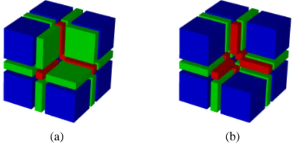
β-simple. The inclusion map i1 : X1 → X0 is therefore a weak homotopy equivalence. If dim(x1) = 0, let y0,y1,y2be the three 2-faces including x1and included in x0. The reader can check in Figure 10 that these three faces are up-unipolar in x↑⋆1 and that x↑⋆1 \ {y0,y1,y2} is a core of x
↑⋆
1 . Hence, x
↑⋆
1 is not contractible and x1is not β-simple.
2.7 γ-simple points
The example set X0 highlights the need for a weaker
condi-tion on points to be deleted when processing a thinning in a
1 2 3 4 5 6 7 8 9 10 11 12 13 14 15 16 17 18 19 20 21 22 23 24 25 26 27 28 29 30 31 32 33 34 35 36 37 38 39 40 41 42 43 44 45 46 47 48 49 50 51 52 53 54 55 56 57 58 59 60
(a) (b)
Fig. 10 (a) The subset x↑⋆1 of X0. (b) The core of x↑⋆1 in X0.
digital image. The following definition of γ-simple points8
and their properties are due to Barmak and Minian [42]. Bertrand [38] defines a quite similar notion.
Property 18 leads to an alternative definition of β-simple points: a point x is β-simple iff xl⋆ is contractible. In turn,
this alternative definition leads to the definition of γ-simple points.
Property 18 ([42, Proposition 3.3]) Let X be a finite poset
and x a point in X. Then xl⋆is contractible iff x↓⋆or x↑⋆is
contractible.
Definition 19 A point x of a poset is a γ-simple point if the
poset xl⋆is homotopically trivial.
As we have observed (see Subsection 2.4) that the ho-motopy groups of a poset are unchanged if we consider the reverse order on X, we can state the following proposition. Proposition 20 Let X be a finite poset and x be a γ-simple
point in X. Then x is γ-simple in X equipped with the reverse order and the dual topology.
Since a contractible space is obviously homotopically trivial, a β-simple point is a γ-simple point. In general, the converse is false as it will appear in Example 24. Neverthe-less, if the length of X is less than or equal to 2 (intuitively, if X is 2-dimensional), then any γ-simple point is a β-simple point [42].
The following property gives a sufficient condition for a point to be γ-simple. This condition enables to decrease the
cost of looking for γ-simple points since the length of x↑⋆
or x↓⋆ is always less than or equal to the length of xl⋆.
Property 21 ([42, Proposition 3.17]) Let X be a finite poset
and x a point in X. Then xl⋆is homotopically trivial if x↓⋆
or x↑⋆is homotopically trivial.
If the length of the space is less than or equal to 3, and x
is neither a maximum nor a minimum, the height of x↑⋆and
8 Barmak and Minian call them γ-points. To be consistent with the
previous subsection, we prefer to call them γ-simple points.
x↓⋆is less than or equal to 1. Hence, if x↑⋆or x↓⋆is
homo-topically trivial, it is contractible. Thanks to Property 18, we
deduce that xl⋆ is contractible and therefore homotopically
trivial.
The next property ensures that the deletion of a γ-simple point does not modify the homotopy groups.
Property 22 ([42]) ([42, Proposition 3.10]) Let X be a finite
poset. Let x ∈ X be a γ-simple point. Then, the inclusion i : X \ {x} → X is a weak homotopy equivalence.
Finally, the following theorem states that, when deleting a γ-point in a finite poset, the homotopy type of the contin-uous analogue is unchanged.
Theorem 23 ([42]) ([42, Theorem 3.15]) Let X be a finite
poset and let x ∈ X be a γ-simple point. Then |K(X \ {x})| and |K(X)| are simple-homotopy equivalent.
In a 3D image X, the cost to decide whether the set xl⋆is
homotopically trivial is not expensive. Indeed, K(xl⋆) is a 2-dimensional simplicial complex and it is enough to compute its connected components and its Euler characteristic. An alternative to look at γ-simple points, in any dimension, is to remove β-simple points in xl⋆until stability. If the result is a
singleton, by Property 15, xl⋆is weak homotopy equivalent
to a point and therefore homotopically trivial. Moreover, the scheme proposed for the deletion of simple points is still valid (γ-simple points with same height can be removed in parallel).
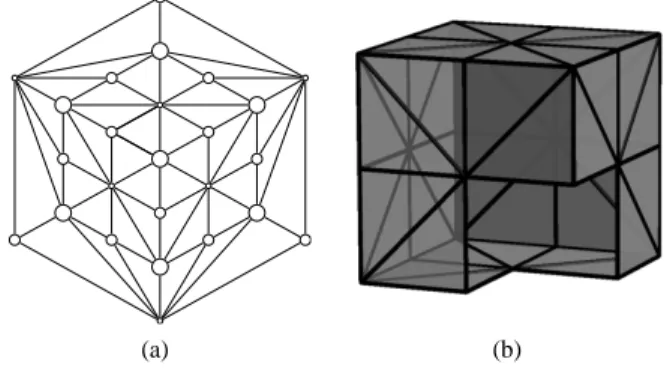
Example 24 Let us consider the test set X0. We have seen that x1is a β-simple point iff dim(x1) ≥ 1. Suppose now that
dim(x1) = 0. The chain complex K(x↑⋆1 ) (see Subsection 2.4) is depicted in Figure 11 in a 2D-space and in a 3D-space. It is clearly contractible, so x↑⋆ is homotopically trivial
(The-orem 4). Thus, x1is a γ-point and the injection i : X1 → X0 is a weak homotopy equivalence.
2.8 Complexes and simplicity
In this subsection, we establish some specific properties of spaces of cubical or simplicial complexes. The proofs of these new results are provided in Appendices B and C.
In Section 4, the proof of Theorem 47 needs the space to have a property that can be understood in the framework of complexes as asking the boundary of a cell with a “large hole” to be homotopically trivial. So, we introduce the fol-lowing definition.
Definition 25 A poset X has the pierced sphere property if,
for any x, y ∈ X such that y covers x, the set x↑⋆ \ {y} is
homotopically trivial. 1 2 3 4 5 6 7 8 9 10 11 12 13 14 15 16 17 18 19 20 21 22 23 24 25 26 27 28 29 30 31 32 33 34 35 36 37 38 39 40 41 42 43 44 45 46 47 48 49 50 51 52 53 54 55 56 57 58 59 60 61
(a) (b)
Fig. 11 (a) The pure simplicial 2-complex K(x↑⋆1 ) in a 2D space. The large/middle/small circles are vertices associated to 3-/2-/1-faces of
x↑⋆1 . (b) The complex K(x↑⋆1 ) in a 3D space. The seven vertices as-sociated to the 3-faces of x↑⋆1 are in corner position and the vertices associated to the 1-faces are in centre position.
The next proposition states that this pierced sphere prop-erty is satisfied by the spaces of cubical or simplicial com-plexes. In Appendix B, we actually prove an extended ver-sion of this statement (Proposition 58).
Proposition 26 Let X be a cubical or a simplicial complex
equipped with the order ⊇. Then, X has the pierced sphere property.
In digital topology, the usual requirement for a point y to be simple for an object Y in a space X (that is a point which can be removed from Y in a topologically sound thinning procedure) is that (i) the inclusion i : Y \ {y} → Y induces a one-to-one correspondence between the connected compo-nents of the object before and after the removal (i.e., Y and
Y \ {y}), (ii) the inclusion i′: X \ Y → (X \ Y) ∪ {y} induces
a one-to-one correspondence between the connected com-ponent of the background before and after the removal (i.e.,
X \ Y and X \ Y ∪ {y}), (iii) the inclusion i induces
isomor-phisms between the fundamental groups of the connected components of the object before and after the removal, (iv)
the inclusion i′induces isomorphisms between the
funda-mental groups of the connected components of the back-ground before and after the removal [43]. In [29], it has been proved, thanks to the linking number borrowed to knots the-ory, that for 3D digital images interpreted with the (6,26) or the (26,6) pair of adjacencies, there is no need to con-sider the fundamental groups of the background since their preservation is implied by the three first conditions. The fol-lowing theorem generalises, in our framework, this property to spaces of any dimension (and, in a certain sense, defined in [22], for any pair of adjacencies).
Theorem 27 Let X be a cubical complex equipped with the
order ⊇ which is also a cubical complex for the dual order
⊆. Let Y be a proper subset of X and y be a β-simple point
in Y. Then y is γ-simple in (X \ Y) ∪ {y}.
l1 l2 . . . lℓ
⊥
Fig. 12 Hasse diagram of the label set L = {li}ℓi=1∪ {⊥}.
Remark 28 We do not know if this theorem remains true in
any dimension if we replace the hypothesis “y is a β-simple point” by “y is a γ-simple point”. Nevertheless, if the di-mension of X is 2, γ-simple points are β-simple points, so it is obviously true in this case. Moreover, we have proved, by checking all configurations with the help of a computer pro-gram, that it is also true in F3, the space of 3-dimensional cubical complexes. In Appendix D, Counterexample 61 pro-vides a case where Theorem 27 is false when the space X is not a complex for the dual order.
3 Label images
Let L be a finite poset with a minimal element, denoted ⊥, and such that two distinct elements in L \ {⊥} are not compa-rable. We set L⋆= L \ {⊥} and we write ℓ for the cardinality
of L⋆. The elements of L⋆are called proto-labels. The Hasse
diagram of the poset L is depicted in Figure 12. A label
dig-ital image is a function defined on Zn, with values in L, and equal to ⊥ everywhere except on a finite set of points of Zn.
Let l ∈ L, l , ⊥ be a proto-label and λ a label digital
image. The set λ−1({l}) is the support of the proto-label l
(in the label digital image λ). The union of the supports of all proto-labels is the domain of the image λ. (This domain is finite by definition.) The set λ−1({⊥}) is the background
of the image λ. The background and the supports define a partition of Zn.
In order to equip the discrete grid on Zn with a
topol-ogy, we enrich this grid by adding low dimensional points between the xels of Zn (for instance, in Z3, we add surfels, linels and pointels) whose purpose is to link the distinct ad-jacent xels and to confer a poset structure to the discrete space. Typically, such a space is the space of cubical com-plexes, Fn, or any poset associated to a cellular
decomposi-tion of the space [44, 45, 46, 47, 48]. Thereby, the label digi-tal images considered in this article are defined on a locally finite poset (X, ≤): we wish to link points of Zn to finitely
many neighbours. Indeed, all sets x↑⋆and x↓⋆which appear
in the definitions of β/γ-simple points will be finite. This will allow us to use the results of Section 2.
Furthermore, we suppose that the embedding of Znin X
puts in one-to-one correspondence the points of Znwith the
minimal points of X. The reader must be aware that this is counterintuitive. For instance, if the poset is the space
of cubical complexes, Fn, this one must be ordered by the
1 2 3 4 5 6 7 8 9 10 11 12 13 14 15 16 17 18 19 20 21 22 23 24 25 26 27 28 29 30 31 32 33 34 35 36 37 38 39 40 41 42 43 44 45 46 47 48 49 50 51 52 53 54 55 56 57 58 59 60
(a) (b) (c)
Fig. 13 Label images. The proto-labels are r, g, b (depicted in red,
green and blue). The other labels are obtained by using the additive colour model (e.g., {r, b} is depicted in magenta) except ⊤ which is depicted in black (⊥ is depicted in white). (a) X is a subset of F2. T
is the power set 2{b,r}. Observe that in this image, there are points of height 0 that have distinct dimensions. (b) X is built from an hexagonal tessellation. T is the power set 2{r,g,b}. The labels of the points of height greater than 0 are assigned according to the rule which will be used in Section 5: a label is the supremum of the labels of the minimal points in the neighbourhood. (c) X is built from a semi-regular tessellation. The labels are given according to the same rule as in (b) but T is not a power set: T = {⊥, r, g, b, ⊤}.
dual of the inclusion, ⊇, i.e., the height of a face is its codi-mension. The reason to do so is to put the xels of Zn, which
contain all the information of the original image, at the same height in the poset, namely “on the floor”. Then, we can add, above those minimal points, the topological “glue” that is needed to interpret the image. Most of the time, the labels of the minimal points will be proto-labels, or ⊥, that is mini-mal labels in T and the image will be non-decreasing. In the
sequel, we identify the points of Zn with their images in X
so the xels are the minimal points of X.
Since we enrich the initial space with low dimensional faces in order to get both a topological space and an alge-braic structure, we are led to do so with the label set to extend the digital label image on these supplementary low dimensional faces. That is why we embed the label set in an atomistic lattice (T, ≤) whose minimum is the embedding of
⊥ and atoms are the embeddings of the proto-labels of L (a
few definitions and properties about lattices can be found in Appendix A). In the sequel, we identify the elements of L with their images in T . We denote by ⊤ the maximum of T . A label is an element of T . Given a (proto-)label set L⋆the smallest lattice T including L is T = L ∪ {⊤}. This is the lattice used by Ronse and Agnus in [49, 50] to define mor-phological operators on label images. The largest atomistic
lattice in which we can embed L is the power set 2L⋆
(with the natural embedding which associates ∅ to ⊥ and the sin-gleton {l} to any proto-label l).
Some ways to associate labels to points in X that are not xels are discussed in [44, 51]. We have proposed, in [22], our own modus operandi to embed a binary digital image
defined on Zn in a binary image defined on Fn. It can be
straightforwardly extended to label images and we use it, in a particular case, in Section 5 but we do not develop more
(a)
(b) (c) (d)
Fig. 14 (a) A label image whose domain is F2and whose codomain
is the power set T = 2{b,r}={∅, {b}, {r}, {b, r}} equipped with the inclu-sion. The points with label {b} are depicted in blue, those with label {r} in red and those with label {b, r} in magenta. The points of the back-ground (label ⊥ = ∅) are depicted in white with a black border or are not depicted. (b) In blue, the support of the label {b}. (c) In red, the support of the label {r}. (d) In magenta, the support of ⊤ = {b, r}.
this issue in this article. This is why we actually just set the following definition for label images.
Definition 29 (Label images) Let X be a locally finite poset
and T an atomistic lattice. A label image is a function µ : X → T .
Figure 13 provides various examples of label images. We have seen that when we start from a label digital
im-age λ : Zn → L and we construct a label image µ : X → T ,
the labels of the minimal points of X (i.e., the xels) are the atoms of T (i.e., the proto-labels). When a label image has this property, we say that this image is pure.
A label image can be seen as a superposition of binary
layers. Indeed, if µ is a label image, and l ∈ L⋆ is a
proto-label, the image µl= µ∧l is a binary image whose codomain
is {⊥, l} (remember that we denote by ∧ and ∨ the infimum and supremum operations of the lattice T : see Appendix A). The next proposition establishes that µ is the supremum of all the binary images µl, l ∈ L⋆.
Proposition 30 Let µ : X → T be a label image. Let L⋆
be the set of atoms of T . Then, µ = W
l∈L⋆µl where, for all l ∈ L⋆, µ
l= µ ∧ l.
Proof We set L⋆={li}ℓi=1. Let x be a point in X. Let A ⊆ L⋆
be the set of atoms in T which are less than or equal to µ(x).
Then, µ(x) = W
a∈Aa for T is atomistic. Let l ∈ L⋆, be an
atom in T . We have (µ ∧ l)(x) = µ(x) ∧ l = (W
a∈Aa) ∧ l. It is
plain that (µ ∧ l)(x) = l iff l ∈ A and (µ ∧ l)(x) = ⊥ iff l < A.
Thus, µ(x) = W
a∈Aa = Wl∈A(µ(x) ∧ l) =Wl∈L⋆(µ(x) ∧ l) =
W
l∈L⋆(µ ∧ l)(x). ⊓⊔
Let µ : X → T be a label image and t be a label. The
support of t in µ is the subset htiµof X equal to {x ∈ X |
µ(x) ∧ t , ⊥}. When there is no ambiguity, we also say the
support of t instead of the support of t in µ and we write
1 2 3 4 5 6 7 8 9 10 11 12 13 14 15 16 17 18 19 20 21 22 23 24 25 26 27 28 29 30 31 32 33 34 35 36 37 38 39 40 41 42 43 44 45 46 47 48 49 50 51 52 53 54 55 56 57 58 59 60 61


![Fig. 4 (From [29]) (a) A cubical 3-complex X. (b) A subcomplex Y.](https://thumb-eu.123doks.com/thumbv2/123doknet/14430752.515131/8.918.499.750.251.351/fig-from-cubical-complex-x-b-subcomplex.webp)