HAL Id: hal-01780844
https://hal.archives-ouvertes.fr/hal-01780844v3
Submitted on 12 Sep 2018
HAL is a multi-disciplinary open access
archive for the deposit and dissemination of
sci-entific research documents, whether they are
pub-lished or not. The documents may come from
teaching and research institutions in France or
abroad, or from public or private research centers.
L’archive ouverte pluridisciplinaire HAL, est
destinée au dépôt et à la diffusion de documents
scientifiques de niveau recherche, publiés ou non,
émanant des établissements d’enseignement et de
recherche français ou étrangers, des laboratoires
publics ou privés.
Christian Doczkal, Damien Pous
To cite this version:
Christian Doczkal, Damien Pous. Treewidth-Two Graphs as a Free Algebra. Mathematical
Founda-tions of Computer Science, Aug 2018, Liverpool, United Kingdom. �10.4230/LIPIcs.MFCS.2018.60�.
�hal-01780844v3�
Christian Doczkal
Univ Lyon, CNRS, ENS de Lyon, UCB Lyon 1, LIP, France [email protected]
Damien Pous
Univ Lyon, CNRS, ENS de Lyon, UCB Lyon 1, LIP, France [email protected]
Abstract
We give a new and elementary proof that the graphs of treewidth at most two can be seen as a free algebra. This result was originally established through an elaborate analysis of the structure of K4-free graphs, ultimately reproving the well-known fact that the graphs of treewidth at
most two are precisely those excluding K4 as a minor. Our new proof is based on a confluent
and terminating rewriting system for term-labeled graphs and does not involve graph minors anymore. The new strategy is simpler and robust in the sense that it can be adapted to subclasses of treewidth-two graphs, e.g., graphs without self-loops.
2012 ACM Subject Classification Mathematics of computing → Graph theory · Theory of com-putation → Rewrite systems · Computing methodologies → Symbolic and algebraic manipulation Keywords and phrases Treewidth, Universal Algebra, Rewriting
Supplement Material http://perso.ens-lyon.fr/damien.pous/covece/tw2rw
Funding This work has been funded by the European Research Council (ERC) under the Eu-ropean Union’s Horizon 2020 programme (CoVeCe, grant agreement No 678157). This work was supported by the LABEX MILYON (ANR-10-LABX-0070) of Université de Lyon, within the program "Investissements d’Avenir" (ANR-11-IDEX-0007) operated by the French National Research Agency (ANR).
1
Introduction
The notion of treewidth [9] is a cornerstone of algorithmic graph theory and parameterised complexity: treewidth measures how close a graph is to a forest, and many problems that can be solved in polynomial time on forests but are NP-complete on arbitrary graphs remain polynomial on classes of graphs of bounded treewidth. This is the case for instance for the graph homomorphism problem (and thus k-coloring) [13, 5, 14].
Similar to trees, graphs of bounded treewidth can be described by a variety of syn-taxes [8]. Among the open problems, there is the question, for graphs of a given treewidth, of finding a syntax making it possible to get a finite and equational axiomatisation of graph isomorphism [8, page 118]. This question was recently answered positively for directed multigraphs of treewidth at most two [7].
The syntax used in [7] is comprised of two binary operations: series and parallel compo-sition [12], their neutral elements, and a unary converse operation. In this syntax, several terms may denote the same graph (up-to isomorphism); the key result of [7] is that the
sponding equational theory is characterized by twelve equational axioms, defining so-called 2p-algebras.
To get this result, the authors define a function t from graphs to terms and establish that t is a isomorphism of 2p-algebras. The function t is defined using an elaborate anal-ysis of the structure of treewidth-two graphs, which requires complicated graph-theoretical arguments that are not directly related to the proposed axiom system. For instance they ultimately reprove the well-known fact that the graphs of treewidth at most two are pre-cisely those graphs excluding K4 (the complete graph with four vertices) as a minor [12]. The authors also make t as canonical as possible in order to facilitate the proof that on isomorphic graphs, t returns terms that are congruent modulo the axioms. This comes at the price of complicating the proofs that t is a homomorphism of 2p-algebras.
In the present paper, we reprove the result from [7] using a completely different approach inspired by [3]: instead of using an elaborate top-down analysis, we design a graph rewriting system on term-labeled graphs and use it to reduce graphs, in a bottom-up fashion, to a shape where a term can be read off. This process is highly nondeterministic but can be shown confluent modulo the axioms. This results in big simplifications: tree decompositions are only used to show that all treewidth-two graphs can be reduced to the point where a term can be read off, and minors are not used at all in this new approach.
Another important feature of this new proof is that it makes it possible to discover the required axioms almost automatically, mainly during the confluence proof. It is also more robust: it allows us to solve two problems left open in [7], characterizing connected graphs as a free-algebra, and characterizing self-loop free graphs as a free-algebra, in both cases for graphs of treewidth at most two.
The first problem was solved recently [16] using a purely model-theoretic argument: 2p-algebras form a conservative extension of 2pdom-2p-algebras, the counterpart of 2p-2p-algebras for connected graphs. Our strategy makes it possible to proceed the other way around: we prove the main result for connected graphs and 2pdom-algebras (Sections 3 to 5), before extending it to potentially disconnected graphs and 2p-algebras using a simple and mainly algebraic argument (Section 6).
The second problem was still open. We solve it using a slight variation of the presented proof, which actually leads us to the discovery of the required axioms (Section 7).
2
Preliminaries: 2p- and 2pdom-algebras
We recall the definitions of 2p- and 2pdom-algebras [7, 16]. We let a, b . . . range over the letters of a fixed alphabet A. We consider labeled directed graphs with two designated vertices. We just call them graphs in the sequel.
IDefinition 1. A graph is a tuple G = hV, E, s, t, l, ι, oi, where V is a finite set of vertices, E is a finite set of edges, s, t : E → V are maps indicating the source and target of each edge, l : E → A is a map indicating the label of each edge, and ι, o ∈ V are the designated vertices, respectively called input and output.
Note that we allow multiple edges between two vertices, as well as self-loops.
IDefinition 2. A homomorphism from G = hV, E, s, t, l, ι, oi to G0= hV0, E0, s0, t0, l0, ι0, o0i is a pair h = hf, gi of functions f : V → V0 and g : E → E0 that respect the various components: s0◦ g = f ◦ s, t0◦ g = f ◦ t, l = l0◦ g, ι0 = f (ι), and o0= f (o).
A (graph) isomorphism is a homomorphism whose two components are bijective func-tions. We write G ' G0 when there exists an isomorphism between graphs G and G0.
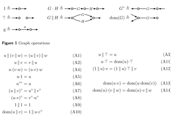
1, G · H , G H G◦, G
> , G k H , G
H
dom(G), G
a , a
Figure 1 Graph operations
u k (v k w) = (u k v) k w (A1)
u k v = v k u (A2)
u·(v·w) = (u·v)·w (A4)
u·1 = u (A5)
u◦◦= u (A6)
(u k v)◦= u◦k v◦ (A7)
(u·v)◦= v◦·u◦ (A8)
1 k 1 = 1 (A9)
dom(u k v) = 1 k u·v◦ (A10)
u k > = u (A3)
u·> = dom(u)·> (A11) (1 k u)·v = (1 k u)·> k v (A12)
dom(u·v) = dom(u·dom(v)) (A13) dom(u)·(v k w) = dom(u)·v k w (A14)
Figure 2 Axioms of 2p-algebras (A1-A12) and 2pdom-algebras (A1,A2,A4-A10,A13,A14)
We consider the following signatures for terms and algebras:
Σ = {·2, k2, _◦1, 10} Σ>= Σ ∪ {>0} Σdom = Σ ∪ {dom1}
We usually omit the · symbol and we assign priorities so that the term (a · (b◦)) k c can be written just as ab◦k c.
Graphs form algebras for those signatures by considering the operations depicted in Figure 1, where input and outputs are represented by unlabelled ingoing and outgoing arrows. The binary operations (·) and ( k ) respectively correspond to series and parallel composition, converse (_◦) just exchanges input and output, and domain (dom(_)) relocates the output to the input.
A graph is called a test if its input and output coincide. The parallel composition of a graph with a test merges the input and output of the former graph. For instance, the graph a k 1 consists of a single vertex with a self-loop labeled with a. Also note that the graph dom(G) is isomorphic to the graph G·> k 1. For Σ>-terms, we will therefore consider dom(u) to be an abbreviation for u> k 1.
IDefinition 3. A 2p-algebra is a Σ>-algebra satisfying axioms A1-A12 from Figure 2. A 2pdom-algebra is a Σdom-algebra satisfying axioms A1,A2,A4-A10,A13,A14 from Figure 2.
ILemma 4. Every 2p-algebra is a 2pdom-algebra (with dom(u) , u> k 1).
Proof. This easy result is implicitly proved in [16]; Coq proofs scripts are available [10]. J
IProposition 5. Graphs (up to isomorphism) form a 2p-algebra.
Given Σ>-terms u, v with variables in A, we write 2p ` u = v when the equation is derivable from the axioms of 2p-algebra (equivalently, when the equation universally holds in all 2p-algebras). Similarly for Σdom-terms and 2pdom-algebras.
By interpreting a letter a ∈ A as the graph a in Figure 1, we can associate a graph g(u) to every term over the considered signatures. By Proposition 5, 2p ` u = v entails g(u) ' g(v) for all Σ>-terms u, v and similarly for Σdom-terms and 2pdom-algebras (using Lemma 4).
IDefinition 7. A Σ>-term u is called a test if 2p ` u k 1 = u. A Σdom-term u is called a test if 2pdom ` u k 1 = u. We write T for the set of tests and N for the set of non-tests. We let α, β, and γ range over terms that are tests.
Thanks to converse being an involution, there is a notion of duality in 2p-algebras: a valid law remains so when swapping the arguments of products and replacing dom(u) with dom(u◦).
ILemma 8. The following laws hold in all 2pdom-algebras. 1. dom(u) k 1 = dom(u) (dom(u) is a test)
2. α◦= α
3. αβ = α k β = βα 4. (u k v)α = u k vα
Proof. As is standard for involutive monoids, we have 1◦= 1 and, therefore, dom(α) = α by (A10). We then reason as follows:
1. dom(u) = dom(u)(1 k 1) = dom(u)1 k 1 = dom(u) k 1 2. α◦= (α k 1)◦= 1 k 1α◦= dom(1 k α) = dom(α) = α
3. By commutativity of k , it suffices to prove the first equation (using Claim (4)): αβ = (α k 1)β = α k 1β = α k β
4. We show the dual: α(u k v) = dom(α)(u k v) = dom(α)u k v = αu k v J
IRemark. Lemma 8 is implicitly proved in [16], and Coq proofs scripts are available [10]. We nevertheless provide a proof here for the sake of completeness. Also note that similar facts were already proven for 2p-algebra in [7] but that we need proofs in 2pdom-algebras here.
ILemma 9 ([7, Proposition 1]). The following laws hold in all 2p-algebras 1. u>v k >w> = u>w>v
2. uv k >w> = (u k >w>)v
3. >u◦> = >u> 4. α>β k u = αuβ
ILemma 10. A Σdom- or Σ>-term u is a test iff g(u) is a test.
Proof. The direction from left to right follows with Proposition 5. The converse direction follows by induction on u using the lemmas above. We show the case for uv. If g(uv) is test, then both g(u) and g(v) must be tests and we have 2pdom ` u k 1 and 2pdom ` v k 1 = v. Thus 2pdom ` uv k 1 = (u k 1)(v k 1) k 1 = (u k 1) k (v k 1) k 1 = (u k 1) k (v k 1) = uv J One useful consequence of the lemma above is that uv is a test iff both u and v are tests and u k v is test if either u or v is a test. Further, A ⊆ N , i.e., letters are non-tests.
We conclude this preliminary section by defining the subalgebra of treewidth-two graphs.
IDefinition 11. A simple graph is a pair hV, Ri consisting of a finite set V of vertices and an irreflexive and symmetric binary relation R on V . The skeleton of a graph G is the simple graph obtained from G by forgetting input, output, labeling, self loops, and edge directions and multiplicities. The strong skeleton of a graph is the skeleton of G with an additional edge connecting ι and o.
IDefinition 12 ([9]). Let G be a simple graph. A tree decomposition of G is a tree T where each node t ∈ T is labeled with a set of vertices Btsuch that:
1. For every vertex x of G, the set of nodes t such that x ∈ Btis nonempty and connected
in T (i.e., forms a subtree)
2. For every xy-edge, there exists some t such that {x, y} ⊆ Bt.
The width of a tree decomposition is the size of its largest set Btminus one, and the treewidth
of a graph is the minimal width of a tree decomposition for this graph. The simple graphs of treewidth at most one are the forests. We write TW2 for the collection of graphs whose strong skeleton has treewidth at most two.
IProposition 13 ([7]). TW2 forms a subalgebra of the Σ>-algebra of graphs.
ICorollary 14. For every term u, g(u) ∈ TW2.
The main results about 2p- and 2pdom-algebras, which we reprove in this paper, are that TW2(up to isomorphism) forms the free 2p-algebra (over A) [7] and that the connected graphs in TW2form the free 2pdom-algebra [16]. As explained in the introduction, we start with the connected case, which we then extend to deal with disconnected graphs.
3
A Confluent Rewriting System for Term-labeled Graphs
The rewriting system we define to extract terms from graphs works on a generalised form of graphs, whose edges are labeled by terms rather than just letters, and whose vertices are labeled by tests.
We work exclusively with Σdom-terms and connected graphs in Sections 3 to 5; for these sections we thus abbreviate 2pdom ` u = v as u ≡ v.
IDefinition 15. A term-labeled graph is a tuple G = hV, E, s, t, l, ι, oi that is a graph except that l is a function from V ] E to Σdom-terms (we assume V and E to always be disjoint) such that l(x) ∈ T for vertices x and l(e) ∈ N for edges e. We write exp(G) for the expansion of G obtained by replacing every edge e with g(l(e)) and every vertex x with g(l(x)). Restricting edge labels to non-tests ensures that replacing edges by the graphs described by their labels does not collapse source and target of the edge. Similarly, replacing vertices by graphs is only meaningful if the replacement is a test.
IExample 16. A term-labeled graph and its expansion:
exp a b cc◦ 1 ef k 1 d k 1 = a b c c d e f
We will compare term-labeled graphs using a notion of isomorphism where labels are compared modulo 2pdom-axioms. A subtlety here is that we should consider as equivalent two graphs where one is obtained from the other by reversing a u-labeled edge and labeling it with u◦ (this operation preserves the expansion). The following predicate, which we use in the definitions below, captures this idea in a formal way: L(x, y, e, u) means that e can be seen as a u-labeled xy-edge, up to ≡.
L(x, y, e, u) , (s(e) = x ∧ t(e) = y ∧ l(e) ≡ u) ∨ (s(e) = y ∧ t(e) = x ∧ l(e) ≡ u◦)
IDefinition 17. Two term-labeled graphs G = hV, E, s, t, l, ι, oi and H = hV0, E0, s0, t0, l0, ι0, o0i are weakly isomorphic, written G ∼= H, if there is a pair of bijective functions hf, gi satisfying
(1) u α v 7→ uαv (2) α u β 7→ α·dom(u·β) (3) u v 7→ u k v (4) u α 7→ α(u k 1)
Figure 3 Rewriting system for term-labeled graphs. The square vertices may have additional
incident edges. The circular vertices (i.e., those that are removed) must be distinct from input and output and may not have other incident edges.
2. For all vertices x ∈ V , l(x) ≡ l0(f (x)).
3. For all edges e ∈ E and e0∈ E0 such that g(e) = e0, L(s0(e0), t0(e0), e0, l(e)).
IExample 18. Weakly isomorphic graphs always have isomorphic expansions. However, the converse is not true: all three graphs below have isomorphic expansions, but only the first two are weakly isomorphic.
a b◦ c 1 1 1 k d ∼ = a b c 1 1 d k 1 6∼ = a(d k 1)b c 1 1
We now define the rewriting system on term-labeled graphs, as depicted in Figure 3.
IDefinition 19. Let G = hV, E, s, t, l, ι, oi be a term-labeled graph. We write G 7→ G0 if G0 can be obtained from G by applying one of the following rules.
1. If l(x) = α, L(x1, x, e1, u) and L(x, x2, e2, v) where x /∈ {ι, o, x1, x2} and e1 and e2 are the only incident edges of x, then replace e1 and e2 with an uαv-labeled edge from x1 to x2and remove x.
2. If l(x) = α, l(y) = β and L(x, y, e, u) where y /∈ {ι, o} and e is the only edge incident to y, then change the label of x to α·dom(u·β) and remove y and e.
3. If L(x, y, e1, u) and L(x, y, e2, v) then replace e1and e2 with a (u k v)-labeled xy-edge. 4. If s(e) = t(e) = x, l(x) = α and l(e) = u, then assign label α(u k 1) to x and remove e. It is straightforward to verify that 7→ preserves the requirements on edge and vertex labels from Definition 15. We write for the reflexive transitive closure of 7→ up to ∼= (i.e., G H iff either G ∼= H or there exists a sequence G ∼= G17→ G2∼= G37→ . . . 7→ Gn∼= H).
ILemma 20. The relation 7→ is terminating.
ILemma 21. If G 7→ G0, then exp(G) ' exp(G0).
ILemma 22. If G ∼= H and G 7→ G0, then there exists H0 such that H 7→ H0 and G0 ∼= H0. We now show that the relation 7→ is locally confluent up to weak isomorphism. The proof is fundamental: while closing the various critical pairs, we rediscover most of the axioms of 2pdom-algebras. Note that for rules (1) and (3) we do not assume that the square vertices are distinct. This introduces some critical pairs (e.g, between rules 3 and 4), but ensures that reductions are preserved in contexts that collapse input and output (Lemma 30 below).
ILemma 23 (Local Confluence). If G1←[ G 7→ G2, then there exist G 0
1 and G02 such that G17→ G01, G27→ G20 and G01∼= G02.
Proof. If the redexes do not overlap, we can reduce G1 and G2 to the same graph in one step. It remains to analyze the critical pairs. The nontrivial interactions are as follows:
u
α β α u β α
Figure 4 Atomic Graphs
Rules 1 and 2 can interact as follows:
uαv γ β ←[ u v γ α β 7→ γ u αdom(vβ) After applying rule 2 on both sides, it suffices to show dom(uαvβ) ≡ dom(uαdom(vβ)), which is an instance of (A13).
Rules 1 and 3 can interact as follows: uαv◦ γ ←[
u v
γ α
7→ γ u k v α
After applying rule 4 on the left and rule 2 on the right, it suffices to show that we have uαv◦k 1 ≡ dom((u k v)α). We prove it as follows using Lemma 8(4) and (A10): dom((u k v)α) ≡ dom(u k vα) ≡ 1 k u(vα)◦≡ uαv◦k 1.
Rules 3 and 4 can interact as follows:
u k v γ ←[ u v γ 7→ v γ(u k 1)
After applying rule 4 on both sides, it suffices to show u k v k 1 ≡ (u k 1)(v k 1). Since v k 1 is a test, this follows with Lemma 8(4) and (A5).
There are a number of other critical pairs that can easily be resolved using (A1)-(A8) (e.g., two overlapping instances of rule 1 that differ in the direction the edges are matched, or overlapping instances of rule 3). Similarly, overlapping instances of rules 2 and 4 remain instances after the first rule has been applied and the resulting graphs only differ in the order of the tests being generated; thus they are weakly isomorphic by Lemma 8(3). J
IProposition 24 (Confluence). If G1 G G2, then there exists H such that G1 H G2.
IDefinition 25. We call a term-labeled graph atomic if it consists of either a single vertex and no edges or two vertices connected by a single edge as depicted in Figure 4. If A is atomic, we write A for the term that can extracted from A, i.e., αuβ, αu◦β, or α for the atoms in Figure 4, from left to right.
ILemma 26. If A G B for some atomic graphs A, B, then A ≡ B.
Proof. We have A ∼= B by Proposition 24, since atomic graphs are irreducible. The claim
then follows by case analysis on A and B. J
4
Reducibility of Term-Graphs
We now show that the rewriting system from the previous section can be used to reduce graphs of the shape g(u) to atomic graphs. As a consequence, we obtain that u ≡ v iff g(u) ' g(v) and, hence, that equivalence of Σdom-terms is decidable.
To show that g(u) reduces to an atomic graph, we define a function computing for every u an equivalent term that can be obtained as A for some atomic graph A. In particular, if u is not a test, it computes “maximal” tests α and β and a non-test v such that u ≡ αvβ.
IDefinition 27. We define a function f from Σdom-terms to T ∪ T × N × T as depicted in Figure 5, as well as functions d_e and b_c interpreting elements of T ∪ T × N × T as atomic
f(u◦) = match f(u) with f(1) = (1) (αu, u0, βu) ⇒ (βu, u0◦, αu)
(γ) ⇒ (γ)
f(u k v) = match f(u), f(v) with f(a) = (1, a, 1)
(αu, u0, βu), (αv, v0, βv) ⇒ (αuαv, u0k v0, βuβv)
(αu, u0, βu), (γ) ⇒ (αuu0βuk γ)
(γ), (αv, v0, βv) ⇒ (γ k αvv0βv)
(γ1), (γ2) ⇒ (γ1γ2)
f(u·v) = match f(u), f(v) with f(dom(u)) = (dom(u))
(αu, u0, βu), (αv, v0, βv) ⇒ (αu, u0βuαvv0, βv)
(αu, u0, βu), (γ) ⇒ (αu, u0, βuγ)
(γ), (αv, v0, βv) ⇒ (γαv, v0, βv)
(γ1), (γ2) ⇒ (γ1γ2)
Figure 5 Test analysis for Σdom-terms
T ∪ T × N × T
Σdom-terms graphs
term-labeled graphs g f b_c d_e exp(_)
Figure 6 Summary of functions between terms and graphs
graphs and terms, respectively: d(α, u, β)e is the graph on the left in Figure 4 and d(α)e is the graph on the right, b(α, u, β)c, αuβ, and b(γ)c , γ. Note that d(α, u, β)e = b(α, u, β)c. A summary of the functions defined so far is given in Figure 6.
ILemma 28. u ≡ bf(u)c.
Proof. By induction on u. The cases for a, 1, and dom(u) are trivial. The case for u◦ follows with Lemma 8(2). We show the case for f(u k v) where f(u) = (αu, u0, βu) and
f(v) = (αv, v0, βv).
bf(u k v)c = αuαv(u0k v0)βuβv
≡ (αuu0βu) k (αvv0βv) Lemma 8(4) and commutativity of k
≡ bf(u)c k bf(v)c
≡ u k v induction hypothesis
The remaining cases are straightforward. J
We now show that g(u) (seen as a term-labeled graph) reduces to df(u)e. To do so, we first extend the graph operations to term-labeled graphs and prove the context lemma below.
IDefinition 29. If a graph G occurs as a term-labeled graph, it is to be read as the graph where every vertex is labeled with 1 (and every edge is labeled with a single letter as before).
We extend the operations ·, k and dom(_) to term-labeled graphs. If two vertices x and y are identified by an operation, we label the resulting vertex with l(x)·l(y).
ILemma 30 (Context Lemma). If G G0, then G k H G0k H, G·H G0·H, H·G H·G0, and dom(G) dom(G0).
Proof. By induction on G G0. First, all operations preserve weak isomorphisms. Second, a redex in G is still a redex in G·H, H·G, and dom(G) since G remains unchanged except that one of its nodes may cease to be input or output. Similarly, a redex in G is also a redex in G k H (even if H is a test: we do not require the square vertices in rules 1 and 3 to be distinct so that redexes are preserved under collapsing input and output). J Note that the converse of Lemma 30 does not hold. For instance, dom(a) (cf. Figure 1) re-duces by rule 2 to a graph G with a single node labeled 1dom(a1). Hence, dom(a) dom(G) since G ∼= dom(G), but a is an atom and thus irreducible.
IProposition 31 (Reducibility). g(u) df(u)e Proof. The proof proceeds by induction on u.
case u k v : We first reduce g(u) and g(v) using the context lemma.
g(u k v) = g(u) k g(v) def. g
df(u)e k g(v) IH, Lemma 30
df(u)e k df(v)e IH, Lemma 30, comm. k We consider several cases.
If f(u) = (γ) and f(v) = (αv, v0, βv), then df(u)e k df(v)e has a single node labeled
γαvβv (up to commutativity of tests) and a single self loop labeled v0. Hence, we can
apply rule 4:
df(u)e k df(v)e d(γαvβv(v0k 1))e ∼= d(γ k αvv0βv)e ∼= df(u k v)e
If f(u) = (αu, u0, βu) and f(v) = (αv, v0, βv) then df(u)e k df(v)e is an instance of rule 3
and we have:
df(u)e k df(v)e d(αuαv, u0k v0, βuβv)e ∼= df(u k v)e
The remaining cases are analogous. case u·v :
g(u·v) = g(u)·g(v) def. g
∼
= df(u)e·df(v)e IH, Lemma 30 (twice)
If f(u) = (αu, u0, βu) and f(v) = (αv, v0, βv) then df(u)e · df(v)e is an instance of rule 1
with the intermediate vertex labeled βuαv. Hence,
df(u)e·df(v)e d(αu, u0βuαvv0, βv)e ∼= df(u·v)e
The cases where either f(u) = (γ) or f(v) = (γ0) are straightforward. case dom(u) :
g(dom(u)) = dom(g(u)) def. g
If f(u) = (γ), there is nothing to show. Otherwise we have f(u) = (αu, u0, βu) and
therefore dom(df(u)e) is an instance of rule 1: dom(df(u)e) d(αudom(u0βu))e ∼= df(dom(u))e
The cases for a and 1 are straightforward (no reduction required). J We can finally characterise the equational theory of 2pdom-algebras:
ITheorem 32. 2pdom ` u = v iff g(u) ' g(v).
Proof. The direction from left to right follows with Proposition 5. For the converse direction, assume g(u) ' g(v). Then g(u) ∼= g(v) and therefore df(u)e ≡ df(v)e by Proposition 31 and Lemma 26. Hence, u ≡ bf(u)c = df(u)e ≡ df(v)e = bf(v)c ≡ v using Lemma 28 twice. J As explained in the introduction we did not use minors to obtain this result. Actually, we did not use tree decompositions either: those arise only in the following section, where we need to characterize the image of the function g. This sharply contrasts with the approach from [7], where both tree decompositions and minors are used to obtain the above characterization.
5
The free 2pdom-algebra
In order to show that the connected graphs in TW2form the free 2p-algebra, it remains to obtain an inverse to g (up to ≡), i.e., we need to extract terms from such graphs. We again make use of the rewriting system.
In a slight abuse of notation, we also write G ∈ TW2to denote that (the strong skeleton of) a term-labeled graph G has treewidth at most two.
ILemma 33 (Preservation). If G ∈ TW2 is a connected term-labeled graph and G 7→ G0, then G0∈ TW2 and G0 is connected.
Proof. Clearly, no rule disconnects the graph. Also, if G 7→ G0, then the strong skeleton of G0 is a minor of the strong skeleton of G and taking minors does not increase treewidth. J
ILemma 34 (Progress). If G ∈ TW2 is a connected term-labeled graph, then either there exists some G0 such that G 7→ G0 or G is atomic.
Proof. W.l.o.g., we can assume that rules 3 and 4 do not apply. Thus, it suffices to show that either ι and o are the only vertices of G or that there is some vertex distinct from input and output that has at most two neighbors. Let T be a tree decomposition of the strong skeleton of G of width at most two, and remove leafs of T that are included in their unique neighbor (T remains a tree-decomposition). If T has only one node (say t) then {ι, o} ⊆ Bt.
Hence, if there is another vertex, it has degree at most two. Otherwise, let t be a leaf and let z be a vertex appearing only in Bt. Without loss of generality, we can assume z /∈ {ι, o}.
(If z = ι then o ∈ Bt, due to the ιo-edge in the strong skeleton; hence, for any other leaf,
neither ι nor o can be the vertex unique to that leaf.) Since z appears only on Btit has at
most two neighbors. J
IDefinition 35. We define a function t0 from connected term-labeled graphs of treewidth at most two to terms as follows: t0(G) , A for some atomic graph such that G 7→∗ A. A suitable atomic graph A can be computed by blindly applying the rules (Lemmas 33 and 34): all choices lead to equivalent terms (Lemma 26). For connected (standard) graphs G, we write t(G) for t0(G0) where G0 is G seen as a term-labeled graph.
ILemma 36. If G ∈ TW2 is a term-labeled graph and G H, then t0(G) ≡ t0(H).
Proof. Follows with Lemma 26. J
As an immediate consequence of the lemma above we also have:
IProposition 37. If G, H ∈ TW2 are are connected and G ' H, then t(G) ≡ t(H). We now show that t and g are inverses up to term equivalence and isomorphism respectively.
IProposition 38. For all Σdom-terms u, t(g(u)) ≡ u.
Proof. We have t(g(u)) ≡ df(u)e = bf(u)c by Proposition 31 and Lemma 36. The claim
then follows with Lemma 28. J
IProposition 39. If G ∈ TW2 is connected, then g(t(G)) ' G.
Proof. We have t(G) = A for some A such that G 7→∗A. Hence, exp(A) ' G (Lemma 21).
The claim follows since g(A) ' exp(A) for all atoms A. J
The function g is a Σdom-homomorphism by definition. By the above results, this is ac-tually an isomorphism between the 2pdom-algebra of connected graphs in TW2 and the (canonically) free 2pdom-algebra of Σdom-terms quotiented by ≡:
ITheorem 40 ([16]). The connected graphs in TW2(with labels in A) form the free 2pdom-algebra (over A).
6
The free 2p-algebra
We now extend the results from the previous section to disconnected graphs. That is, we show that the class of all graphs in TW2 forms the free 2p-algebra [7]. We use for that the previous function t to extract terms from the various connected components of a graph.
In this section, we take u ≡ v to mean 2p ` u = v. Recall that 2p ` u = v whenever 2pdom ` u = v (Lemma 4). Hence, all the lemmas from the previous section still apply.
IDefinition 41. Let G be a graph. For vertices x, y of G, we write G[x, y] for the graph G with input set to x and output set to y. We abbreviate G[x, x] as G[x]. Further, we write Gxfor the connected component of x (as a subgraph of G, with input and output set to x).
IDefinition 42. Let C(G) be the collection of components Gxobtained by choosing some
vertex x for every connected component of G containing neither ι nor o. We define a function t>extracting terms from (possibly disconnected) graphs as follows:
cG, n H∈C(G) >·t(H)·> t>(G), ( t(Gι)·>·t(Go) k cG ι and o disconnected
t(Gι[ι, o]) k cG ι and o connected
Note that the function t>needs to choose shared input/outputs vertices for all disconnected components. For isomorphic arguments, these choices can differ. We begin by showing that this choice does not matter up to term equivalence.
ILemma 43. Let G ∈ TW2 be a connected test and let x be a neighbor of ι in G. We have t(G)·> ≡ t(G[ι, x])·>.
Proof. Since G ∈ TW2, so is G[ι, x]. Hence, G[ι, x] d(α, u, β)e for some terms α,β, and u. Since G = dom(G[ι, x]), we also have G dom(d(α, u, β)e) by Lemma 30. Moreover, dom(d(α, u, β)e) d(α·dom(uβ))e by rule 2. We reason as follows:
t(G)·> ≡ t0(d(α·dom(uβ))e)·> Lemma 36 = (α·dom(uβ))·>
≡ αuβ·> (A11)
= t0(d(α, u, β)e)·>
≡ t(G[ι, x])·> Lemma 36 J
ILemma 44. Let G ∈ TW2 be a connected graph and let x, y be vertices of G. We have >·t(G[x])·> ≡ >·t(G[y])·>
Proof. Since G is connected, it suffices to show the property for all xy-edges of G. We have
>·t(G[x])·> ≡ >·t(G[x, y])·> Lemma 43 ≡ >·t(G[y, x])◦·> t is a homomorphism
≡ >·t(G[y, x])·> Lemma 9(3)
≡ >·t(G[y])·> Lemma 43
J
Lemmas 44 and 43 also appear in [7]. We remark that the proof of Lemma 43 given here, which depends on the definition of t, is considerably simpler than the one in [7]. The proof of Lemma 44 remains essentially unchanged.
IProposition 45. Let G, H ∈ TW2. If G ' H, then t>(G) ≡ t>(H).
Proof. Follows with Proposition 37 and Lemma 44. J
IProposition 46. g(t>(G)) ' G.
ILemma 47. t>is a homomorphism of 2p-algebras.
Proof. We already showed that that t>respects graph isomorphisms. It remains to show that t>commutes with all operations.
We show t>(G·H) ≡ t>(G)·t>(H). Let F , G·H. We distinguish four cases based on whether ι and o are connected in G and H respectively.
ι and o disconnected in both G and H: In that case, Go and Hι are merged into one
component of F that is connected neither to the input nor to the output of F . By Lemma 44 and Proposition 37 we therefore have: cF ≡ (>t(Go·Hι)>) k cGk cH. We
reason as follows:
t>(F ) ≡ t(Fι)·>·t(Fo) k cF ι and o disconnected in F
≡ t(Gι)·>·t(Ho) k >·t(Go·Hι)·> k cGk cH Fι' Gι, Fo' Go
≡ t(Gι)·>·t(Go·Hι)·>·t(Ho) k cGk cH Lemma 9(1)
≡ t(Gι)·>·t(Go)·t(Hι)·>·t(Ho) k cGk cH t is a homomorphim
ι and o connected in G but not in H: We have cF ≡ cGk cH by Prop. 37 and Lemma 44.
t>(F ) ≡ t(Fι)·>·t(Fo) k cF
≡ t(dom(Gι[ι, o]·Hι))·>·t(Ho) k cF Fι' dom(Gι[ι, o] · Hι), Fo' Ho
≡ t(Gι[ι, o])·t(Hι)·>·t(Ho) k cF (A11), t is a homomorphism
≡ t(Gι[ι, o])·t(Hι)·>·t(Ho) k cGk cH
≡ t>(G)·t>(H) Lemma 9(2) and its dual
The case where input and output are connected only in H is symmetric and the case where they are connected in both graphs follows from t being a homomorphism. Proving that t>commutes with the other operations is done in a similar manner. J
IProposition 48. For all Σ>-terms u, t>(g(u)) ≡ u.
Proof. By induction on u, using Lemma 47. J
ITheorem 49 ([7]). The graphs in TW2(with labels in A) form the free 2p-algebra (over A).
7
1-free 2p-algebras
We now show that the techniques from the previous sections can be adapted to the setting where 1 (and hence dom(_)) are removed from the signature. We define algebras over the signature Σ−1> , Σ>\ {1}, which we call 1-free 2p-algebras, and show that the graphs of treewidth at most two without self-loops and with distinct input and output form the free 1-free 2p-algebra (over A).
The axioms for 1-free 2p-algebras are A1-A4,A6-A8 plus the following three axioms:
(u·v k w)·> = (u k w·v◦)·> (A15)
u·(v·> k w) = (u k >·v◦)·w (A16)
u·v k >·w = u·(v k >·w) (A17)
The main complication in adapting our techniques to the 1-free case is that the syntax of 1-free 2p-algebras cannot express tests, even though the algebra of graphs still exhibits tests-like structures. For instance, if G is a test without self-loops, then G·> is a graph of the proposed free 1-free 2p-algebra. To account for this, we distinguish between the type of Σ−1> -terms, written Tm, and a type of (syntactic) tests defined as follows:
α ∈ Tst ::= 1 | [u] (u ∈ Tm)
Tests, which are not terms, allow us to describe graphs that are tests. We let α,β,. . . range over tests, and we extend the definition of g to tests by setting g(1) = 1 and g([u]) = dom(g(u)). Intuitively, in a test [u], the output of the term u does not matter: u will always be used in contexts where this information disappears, e.g., as in u>; this allows us to treat [u] essentially like dom(u). It also motivates the following notion of equivalence for tests: 1 ≡ 1, and [u] ≡ [v] if u·> ≡ v·>.
We extend the sequential composition to take one or two tests as arguments in a manner that 1 is the neutral element on both sides:
1·v, v u·1 , u 1·α, α
[u]·v, u> k v u·[v] , u k >v◦ [u]·1, [u] [u]·[v], [u> k v]
Note that α·β is a test whereas all other variants are terms. The three operations above appropriately preserve test equivalence (e.g., if α ≡ β, then uα ≡ uβ, αu ≡ βu, γα ≡ γβ, αγ ≡ βγ for all terms u and tests γ.
The definitions above essentially yield a 2-sorted extension of 1-free 2p-algebras. We prove various laws, including all axioms of 2pdom-algebras that can still be expressed in the 2-sorted setting (using [_] instead of dom(_)). Examples of laws that cannot be expressed in the 2-sorted setting are dom(α) ≡ α, and dom(u k v) ≡ 1 k uv◦.
ILemma 51. We have the following equivalences: 1. u> ≡ [u]> and >u ≡ >[u◦].
2. (αu)◦≡ u◦α, (uα)◦≡ αu◦. 3. (xy)z ≡ x(yz)
(for all x, y, z either test or term).
4. [uv] ≡ [u[v]] 5. αβ ≡ βα
6. α(v k w) ≡ αv k w. 7. [uv k w] ≡ [u k wv◦].
Proof. For all statements involving tests α of unknown shape, we distinguish the cases α = 1 (usually trivial) and α = [w] for some w. Claims (1) and (2) are straightforward. By (2) and the laws for converse, we only need to consider 5 of the 8 cases of (3). (uα)v ≡ u(αv) follows with (A16) and (uv)α ≡ u(αv) follows with (A17). For (αβ)γ ≡ α(βγ) we repeatedly use (A15) with v = >. The remaining cases for associativity are straightforward. Claims (4) and (5) follow with associativity. Claim (6) follows with (A1). Claim (7) follows with (A15). J Having recovered most of the laws of 2pdom-algebras, we adapt the rewriting system for 2pdom-algebras (Figure 3) to the 1-free case. We define term-labeled graphs as for 2pdom, with the difference that now vertices are labeled with syntactic tests and edges are labeled with Σ−1> -terms (whose graphs are never tests). The rewriting system on term-labeled graphs (Figure 3) is adapted by replacing dom(u) with [u], removing rule 4, and restricting rules 1 and 3 such that the two outer vertices must be distinct. For rule 1, this is necessary to avoid introducing self loops.
Local confluence adapts, although for one of the pairs we now need two reduction steps to join the two alternatives.
ILemma 52 (Local Confluence). If G1←[ G 7→ G2, then there exist G01 and G02 such that G1 G01, G2 G20 and G01∼= G02.
Proof. The only interesting (new) critical pair is that of overlapping instances of rule 1, where the outer nodes are the same. Due to the restriction that the outer nodes of rule 1 must be distinct, this pair can no longer be joined by applying rule 1. Instead we use rules 3 and 2 as follows: uαv k w γ β ←[ uαv w γ β ←[ v u w α β γ 7→ u wβv◦ γ α 7→ u k wβv ◦ γ α
After applying rule 2 on both sides, it suffices to show [(uαv k w)β] ≡ [(u k wβv◦)α]. This
In order to adapt Proposition 31, we need to restrict to terms u such that g(u) is con-nected. We write Tm0 and Tst0 for the set of terms and tests respectively, where tests and the extended sequential composition are treated as primitive and > does not occur. We then employ a function f : Tm0 → Tst0× Tm0× Tst0 that can be seen as a type directed variant of the function in Figure 5.
f(a) = (1, a, 1)
f(u◦) = let (αu, u0, βu) := f(u) in (βu, u0◦, αu)
f(u k v) = let (αu, u0, βu), (αv, v0, βv) := f(u), f(v) in (αuαv, u0k v0, βuβv)
f(u·v) = let (αu, u0, βu), (αv, v0, βv) := f(u), f(v) in (αu, u0βuαvv0, βv)
f(γ·u) = let (αu, u0, βu) := f(u) in (γαu, u0, βu)
f(u·γ) = let (αu, u0, βu) := f(u) in (αu, u0, βuγ)
ILemma 53. If u ∈ Tm0 and α ∈ Tst0, then g(u) dfue and g(α) d(α)e.
Proof. We have a context lemma similar to Lemma 30. The proof then proceeds by mutual induction on u and α. The cases correspond to those of Proposition 31. We show two representative cases:
Case u = α · v: We reason as follows.
g(γ · v) ∼= g(γ) · g(v) def. of γ · v
d(γ)e · df ve IH on γ and v, context lemma = d(γ)e · d(αv, v0, βv)e f v = (αv, v0, βv) ≡ v
= d(γαv, v0, βv)e
= df (γ · v)e
Case α = [u]: We reason as follows.
g([u]) = dom(g(u)) def. g
dom(df ue) IH on u, context lemma
= dom(d(αu, u0, βu)e) f u = (αu, u0, βu) ≡ u
7→ d(αu[u0βu])e rule 2
∼ = d([u])e
The remaining cases are analogous. J
We define two extraction functions t1 and t2, where t1 extracts syntactic tests (in Tst0) from graphs that are tests and t2extracts terms (in Tm0) from non-tests. Both functions are defined just like t (Definition 35), exploiting the fact that the rewriting system does not merge or delete input and output. Propositions 38 and 39 then adapt without conceptual changes.
IProposition 54. 1. t1(g(α)) ≡ α for all α ∈ Tst0 and t2(g(u)) ≡ u for all u ∈ Tm0. 2. If G ∈ TW2 is a connected test without self loops, then g(t1(G)) ' G.
3. If G ∈ TW2 is a connected non-test without self loops, then g(t2(G)) ' G.
Using t1 and t2, we define a variant of t>extracting Σ−1> -terms from non-tests without self-loops.
IDefinition 55. Let C(G) as in Definition 42. We define cG , n H∈C(G) >·t1(H)·> t>(G), ( t1(Gι)·>·t1(Go) k cG ι and o disconnected
t2(Gι[ι, o]) k cG ι and o connected
That t>respects graph isomorphisms is immediate with Proposition 54. To show t>is a homomorphism of 1-free 2p-algebras, we require a 2-sorted analog to Lemma 9.
ILemma 56. We have the following equivalences: 1. >u◦> ≡ >u>.
2. αv ≡ α> k v. 3. α>β ≡ α> k >β
4. uv k >α> ≡ (u k >α>)v 5. α>β k >γ> ≡ α>γ>β
Note that, due to Lemma 51(1), any equivalence where a test α appears either only as α> or only as >α (i.e., in α in Lemma 56(4)), also holds if α is replaced by a term.
The remaining proofs of Section 6 adapt to the 1-free setting by carefully distinguish-ing between terms and tests, but without any conceptual changes. For instance, we have t1(G)> ≡ t2(G[ι, x])> for neighbors x of ι.
ITheorem 57. The graphs (with labels in A) of treewidth at most two, with distinct input and output, and without self-loops form the free 1-free 2p-algebra (over A).
The axioms we listed for 1-free 2p-algebras are precisely those needed to prove the 2-sorted 2pdom- and 2p-laws. The proofs of Lemmas 51 and 56 have been verified in the Coq proof assistant [6]. We also used the model generator Mace4 [15] to verify that the axioms of 1-free 2p-algebras are independent. The corresponding scripts can be downloaded from [10].
8
Conclusion and directions for future work
We have proved that graphs in TW2, connected graphs in TW2, and self-loop free graphs in TW2 with distinct input and output respectively form the free 2p-algebra, the free 2pdom-algebra, and the free 1-free 2p-algebra.
To do so, we used a graph rewriting system that makes it possible to extract terms from connected graphs in TW2, in a bottom-up fashion. This technique is much easier than the one used in [7] in that it is more local and does not require us to study the precise structure of graphs in TW2(i.e., through excluded minors).
As explained in the introduction, the result about connected graphs can be reduced to the one about arbitrary graphs by model-theoretic means: one can easily embed a 2pdom-algebra into a 2p-algebra [16], so that 2p-algebras form a conservative extension of 2pdom-algebras. As a corollary of Theorem 57, we get that 2p-algebras also form a conservative extension of 1-free 2p-algebras. It is however unclear how to prove this result directly, by model-theoretic means: terms which are missing in 1-free 2p-algebras (self-loops) can occur deep inside terms of 2p-algebras, unlike terms which are missing in 2pdom-algebras (disconnected components).
As a natural follow-up to this work, we would like to study whether one can character-ize the classes of graphs of higher treewidth as free algebras. The present approach seems promising for treewidth at most three: a reasonable rewriting system is known for recog-nising such graphs [2]. In contrast, trying to exploit the four excluded minors known to characterize treewidth three [4, 2] seems extremely difficult. For larger treewidth, rewriting systems recognizing graphs of a given treewidth can be shown to exist [1]. However, the result is nonconstructive in the same way as the existence of a finite set of excluded minors for each treewidth [17]).
References
1 S. Arnborg, B. Courcelle, A. Proskurowski, and D. Seese. An algebraic theory of graph reduction. Journal of the ACM, 40(5):1134–1164, 1993.
2 S. Arnborg and A. Proskurowski. Characterization and recognition of partial 3-trees. SIAM J. Algebraic Discrete Methods, 7(2):305–314, Apr. 1986.
3 S. Arnborg and A. Proskurowski. Canonical representations of partial 2- and 3-trees. In Proc. SAWT, pages 310–319. Springer, 1990.
4 S. Arnborg, A. Proskurowski, and D. G. Corneil. Forbidden minors characterization of partial 3-trees. Discrete Mathematics, 80(1):1–19, 1990.
5 C. Chekuri and A. Rajaraman. Conjunctive query containment revisited. Theoretical Computer Science, 239(2):211–229, 2000.
6 Coq team. The Coq proof assistant.
7 E. Cosme-Llópez and D. Pous. K4-free graphs as a free algebra. In Proc. MFCS, volume 83
of LIPIcs. Schloss Dagstuhl, 2017.
8 B. Courcelle and J. Engelfriet. Graph Structure and Monadic Second-Order Logic - A Language-Theoretic Approach, volume 138 of Encyclopedia of mathematics and its applica-tions. Cambridge Univ. Press, 2012.
9 R. Diestel. Graph Theory. Graduate Texts in Mathematics. Springer, 2005.
10 C. Doczkal and D. Pous. Supplementary material accompanying this paper. http:// perso.ens-lyon.fr/damien.pous/covece/tw2rw.
11 C. Doczkal and D. Pous. Treewidth-two graphs as a free algebra. In Proc. MFCS, volume 117 of LIPIcs, pages 60:1–60:15. Schloss Dagstuhl, 2018.
12 R. Duffin. Topology of series-parallel networks. Journal of Mathematical Analysis and Applications, 10(2):303–318, 1965.
13 E. C. Freuder. Complexity of k-tree structured constraint satisfaction problems. In Proc. NCAI, pages 4–9. AAAI Press / The MIT Press, 1990.
14 M. Grohe. The complexity of homomorphism and constraint satisfaction problems seen from the other side. Journal of the ACM, 54(1):1:1–1:24, 2007.
15 W. McCune. Prover9 and Mace4, 2005–2010.
16 D. Pous and V. Vignudelli. Allegories: decidability and graph homomorphisms, 2018. to appear in Proc. LiCS 2018.
17 N. Robertson and P. Seymour. Graph minors. XX. Wagner’s conjecture. Journal of Com-binatorial Theory, Series B, 92(2):325 – 357, 2004.