An Optimal Control Problem of Unmanned Aerial Vehicle

HAL Id: hal-03033994

https://hal.archives-ouvertes.fr/hal-03033994

Submitted on 2 Dec 2020

HAL is a multi-disciplinary open access

archive for the deposit and dissemination of

sci-entific research documents, whether they are

pub-lished or not. The documents may come from

teaching and research institutions in France or

abroad, or from public or private research centers.

L’archive ouverte pluridisciplinaire HAL, est

destinée au dépôt et à la diffusion de documents

scientifiques de niveau recherche, publiés ou non,

émanant des établissements d’enseignement et de

recherche français ou étrangers, des laboratoires

publics ou privés.

An Optimal Control Problem of Unmanned Aerial

Vehicle

Kahina Louadj, Fethi Demim, Abdelkrim Nemra, Philippe Marthon

To cite this version:

Kahina Louadj, Fethi Demim, Abdelkrim Nemra, Philippe Marthon. An Optimal Control Problem of

Unmanned Aerial Vehicle. 5th International Conference on Control, Decision and Information

Tech-nologies (CoDIT 2018), Apr 2018, Thessaloniki, Greece. pp.751–756, �10.1109/CoDIT.2018.8394830�.

�hal-03033994�

An Optimal Control Problem of Unmanned Aerial Vehicle

Kahina LOUADJ 1,3_{, Fethi DEMIM} 2

, Abdelkrim NEMRA 2

and Philippe MARTHON 3

Abstract— An unmanned aerial vehicle (UAV) has grown rapidly the last years. They are being engaged in many types of missions, ranging from military to agriculture passing from entertainment and rescue or even delivery. This work consist to ensure the convergence of positions and yaw angle, to their desired trajectories while maintaining stability of roll and pitch angle. For this, formulate this problem to an optimal control problem which minimizes the distance between state and desired state in free final time. Our contribution is to use the Bocop software to solve this problem. And to implement Shooting method with Matlab software.

I. INTRODUCTION

Unmanned Aerial Vehicles (UAV) commonly called ”Drones” [1], [2], [3]; since the earliest days of aviation, their use has increased dramatically in the first decade of the21st_{century, as they have many advantages compared to} air vehicles conventional fixed wings. They can take off and land vertically in limited spaces and easily hover above of the target, which allows their use in any which ground, to the opposition of fixed-wing aircraft, which require prepared tracks for them to taking off and to land. Drones can be used for everything from law enforcement, to search and rescue after natural disasters, weather research, pest control, and even for taking aerial shots for real estate developers. There are several types of drones, in this paper, we are interested in the quad-rotor kind, the choice of this type of drone is motivated by the simplicity of mechanics which facilitates its maintenance, its small size which let fly near obstacles and its dynamic that represents a very attractive control problem [4], [6]. Indeed, these drones are unstable in open loop, hence to drive them, it is necessary to stabilize them using a control algorithm in closed loop.

In our case, We choose quad-rotors drone which is handy, allow vertical takeoff and landing, as well as flying in hard to- Reach areas. The disadvantages are its mass and the con-sumption of energy caused by motors. The drone can perform three flight modes; hover, vertical flight and translation flight. In our work, we are interested in a translation flight that corresponds to the navigation on a horizontal plane, it is ensured by basing itself on pitch and roll tilting movements [25].

In the present study, we consider an optimal control problem of quad-rotor. In order to illustrate this study, we consider distance minimization problem between state and desired state in free final time. To solve this problem we will use the principle of Pontryaguin [18], [19], [24], [26], and determine the optimality equations resulting from this principle; i.e.; a differential-algebraic system as the state equation is provided

*K.Louadj, F.Demim, A.Nemra, P.Marthon

1

Universit´e de Bouira. D´epartement de Math´ematiques. Bouira. Alg´erie.

louadj kahina@yahoo.fr

2

Laboratoire Robotique et Productique, Ecole Militaire Polytechnique, Bordj El Bahri,BP 17, 16111, Alger. Alg´erie.

demifethi@gmail.com, karim nemra@yahoo.fr

3

IRIT-ENSEEIHT. Toulouse, France.

Philippe.Marthon@enseeiht.fr

and the adjoint equation. Thus, in order to determine the initial condition of the adjoint state; we use Bocop software [28] to ensure the convergence of this method. The work presented in this paper is organized as follows : In section I, a dynamic model of the quad-rotor is considered. In section II, implementation of the Shooting method with Matlab software. Finally, discussion, simulation results and conclusion are provided in Section III.

II. QUAD-ROTOR FLIGHT MODEL

Let

X = [φ, ˙φ, θ; ˙θ, ψ, ˙ψ, x, ˙x, y, ˙y, z, ˙z]T ₍₁₎ The model dynamic of the quad-rotor is given under the state space as ˙x = f (x) + g(x, u) considering X = [x1, x2, x3, x4, x5, x6, x7, x9, x10, x11, x12]T, and u = [u1, u2, u3, u4]T be the state, the control vector of the system respectively is given as follows:

                                             ˙x1= x2, ˙x2= a1x4x6+ a2x4Ω + b1u1, ˙x3= x4, ˙x4= a3x2x6+ a4x2Ω + b2u2, ˙x5= x6, ˙x6= a5x2x4+ b3u3, ˙x7= x8,

˙x8= u_m4(cosx1sinx3cosx5+ sinx1sinx5), ˙x9= x10,

˙x10= u_m4(cosx1sinx3sinx5− sinx1cosx5), ˙x11= x12, ˙x12= cosx1_mcosx3u4− g, −π/2 ≤ x1≤ π/2, −π/2 ≤ x3≤ π/2, −π ≤ x5≤ π, xi(0) = 0, i = 1, 12, −20 ≤ uj≤ 20, j = 1, 4, 0 ≤ u4≤ 20. (2) Where g(m/s2 ) :gravity acceleration;Ix, Iy, Iz(kg/m 2

) :roll, pitch and yaw inertia moments respectively,Jr(kg/m

2

) : the rotor inertia; m(kg) : mass;x, y, z(m) : longitudinal, lateral and vertical motions respectively; φ, θ, ψ(rad) : roll, pitch and yaw angles, respectively; wk(rad/s) : rotor angular velocity, where, k equal to 1, 2, 3 and 4; d(m) : the distance between the quadrotor center of mass and the propeller rotation axis; u1, u2, u3(N.m) : aerodynamical roll, pitch and yaw moments respectively;u4(N ) : lift force.

WithΩ = w1− w2+ w3− w4,a1= Iy−Iz Ix ,a2= −Jr Ix ,a3= Iz−Ix Iy ,a4= Jr Iy,a5= Ix−Iy Iz ,b1= d Ix,b2= d Iy,b3= d Iz.

The one of the main objectives of this paper is to find control which ensure the convergence of positions{x, y, z} and yaw angle ψ, to their desired trajectories respectively {xd, yd, zd}, and yaw angle ψd while maintaining stability of roll and pitch angle{φ, θ} in free final time.

Then, the criterion is formulate as follows: J = tf Z 0 (1 ρ(x5−ψd) 2 +(x7−xd) 2 +(x9−yd) 2 +(x11−zd) 2 dt (3) where tf(second) : free final time ; {xd, yd, zd} : desired trajectory of{x, y, z}; ψd: desired trajectory of ψ.

III. SHOOTINGINDIRECT METHOD

The shooting indirect method is used to obtain the value of p(0) necessary to the solution of the problem characterized by the Pontryaguin principle. If it is possible, from the condition of minimization of the Hamiltonian to express the control extremal function of (x(t), p(t)) then the extremal system is a differential system of the form ˙υ(t) = G(t, υ(t)) whereυ(t) = (x(t), p(t)).

The Hamiltonian of the system 2 is given by:

H = p1x2 + p2(a1x4x6 + a2x4Ω + b1u1) + p3(x4) + p4(a3x2x6+ a4x2Ω + b2u2) + p5(x6) + p6(a5x2x4+ b3u3) + p7(x8) + p8(u_m4(cosx1sinx3cosx5 + sinx1sinx5)) + p9(x10) + p10(u_m4(cosx1sinx3sinx5 − sinx1cosx5)) + p11(x12) + p12(cosx1_mcosx3u4− g) +

1

ρ[(x5− ψd)2+ (x7− xd)2+ (x9− yd)2+ (x11− zd)2].

The Euler-Lagrange equations leads to:                                                                                                                    ˙x1= _∂p∂H 1 = x2, ˙x2= _∂p∂H 2 = a1x4x6+ a2x4Ω + b1u1, ˙x3= _∂p∂H 3 = x4, ˙x4= _∂p∂H 4 = a3x2x6+ a4x2Ω + b2u2, ˙x5= _∂p∂H 5 = x6, ˙x6= _∂p∂H 6 = a5x2x4+ b3u3, ˙x7= _∂p∂H 7 = x8, ˙x8= _∂p∂H 8 = u4

m(cosx1sinx3cosx5+ sinx1sinx5), ˙x9= _∂p∂H

9 = x10,

˙x10= _∂p∂H

10 =

u4

m(cosx1sinx3sinx5− sinx1cosx5), ˙x11= _∂p∂H 11 = x12, ˙x12= _∂p∂H 12 = cosx1cosx3 m u4− g, ˙p1= −_∂x∂H 1 = −p8 u4

m(−sinx1sinx3cosx5+ cosx1sinx5) −p10u_m4(−sinx1sinx3sinx5− cosx1cosx5)

−p12(−sinx_m1cosx3u4), ˙p2= −_∂x∂H 2 = −p1− p4(a3x6+ a4Ω) − p6(a5x4), ˙p3= −_∂x∂H 3 = −p8 u4

m(cosx1cosx3cosx5)

−p10(u_m4(cosx1cosx3sinx5) − p12(−cosx_m1sinx3u4), ˙p4= −_∂x∂H

4 = −p2(a1x6+ a2Ω) − p3− p6(a5x2)

˙p5= −_∂x∂H

5 = −p8

u4

m(−cosx1sinx3sinx5+ sinx1sinx5) −p10u_m4(cosx1sinx3sinx5+ sinx1cosx5) −

2 ρ(x5− ψd), ˙p6= −_∂x∂H 6 = −p2(a1x4) − p4(a3x2) − p5, ˙p7= −_∂x∂H 7 = − 2 ρ(x7− xd), ˙p8= −_∂x∂H 8 = −p7, ˙p9= −_∂x∂H 9 = − 2 ρ(x9− yd), ˙p10= −_∂x∂H 10 = −p9, ˙p11= −_∂x∂H 11 = − 2 ρ(x11− zd), ˙p12= −_∂x∂H 12 = −p11, (4)

Let us defined a control law:                  ∂H ∂u1 = p2b1+ 1 2ρu1, ∂H ∂u2 = p4b2+ 1 2ρu2, ∂H ∂u3 = p6b3+ 1 2ρu3, ∂H ∂u4 = p8

m(cosx1sinx3cosx5+ sinx1sinx5) +p10

m(cosx1sinx3sinx5− sinx1cosx5) + p12(cosx1_mcosx3) +1

2ρu4,

(5) Then, the control is:

               u1= − 1 2ρp1b1, u2= − 1 2ρp4b2, u3= − 1 2ρp6b3, u4= 1 2ρ( p8

m(cosx1sinx3cosx5+ sinx1sinx5) +p10

m(cosx1sinx3sinx5− sinx1cosx5) +p12(cosx1_mcosx3)),

(6)

The transversality condition of the Hamiltonian is defined as follows:

H(tf, xi, pi, uj, i = 1, 12, j = 1, 4) = 0 (7) To implement Shooting method, consider|uj| ≤ 1, j = 1, 4. Then, we have to solve the following system :

                                                                                                   ˙υ1= υ2, ˙υ2= a1υ4υ6+ a2υ4Ω + b1u1, ˙υ3= υ4, ˙υ4= a3υ2υ6+ a4υ2Ω + b2u2, ˙υ5= υ6, ˙υ6= a5υ2υ4+ b3u3, ˙υ7= υ8,

˙υ8= u_m4(cosυ1sinυ3cosυ5+ sinυ1sinυ5), ˙υ9= x10,

˙υ10= u_m4(cosυ1sinυ3sinυ5− sinυ1cosυ5), ˙υ11= υ12,

˙υ12= cosυ1_mcosυ3u4− g,

˙υ13= −υ20u_m4(−sinυ1sinυ3cosυ5+ cosυ1sinυ5) −υ22u_m4(−sinυ1sinυ3sinυ5− cosυ1cosυ5) −υ24(−sinυ_m1cosυ3u4),

˙υ14= −υ13− υ16(a3υ6+ a4Ω) − υ18(a5υ4), ˙υ15= −υ20u_m4(cosυ1cosυ3cosυ5)

−υ22(u_m4(cosυ1cosυ3sinυ5) − υ24(−cosυ_m1sinυ3u4), ˙υ16= −υ14(a1υ6+ a2Ω) − υ18− υ18(a5υ2) ˙υ17= −υ20u_m4(−cosυ1sinυ3sinυ5+ sinυ1sinυ5) −υ22u_m4(cosυ1sinυ3sinυ5+ sinυ1cosυ5) −

2 ρ(υ5− ψd), ˙υ18= −υ14(a1υ4) − υ16(a3υ2) − υ17, ˙υ19= − 2 ρ(υ7− xd), ˙υ20= −υ19, ˙υ21= − 2 ρ(υ9− yd), ˙υ22= −υ21, ˙υ23= − 2 ρ(υ11− zd), ˙υ24= −υ23, υi(0) ∈ R, i = 1, 24 (8) Let υ(t, xi, pi, i = 1, 12) be the solution of the previous system at timet with the initial condition (υi(0), i = 1, 24). We construct a shooting function given by:

(a)

(b)

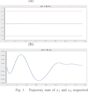
Fig. 1. Trajectory state of x1and x2respectively .

(a)

(b)

Fig. 2. Trajectory state of x3and x4respectively .

ϕ(p) =     υ5(tf, xi, pi, i = 1, 12) υ7(tf, xi, pi, i = 1, 12) υ9(tf, xi, pi, i = 1, 12) υ11(tf, xi, pi, i = 1, 12) − 2    

In the solution, we used the Newton’s method.The solution of ϕ(p(0)) = 0 is to find p(0) such that ϕ(p(0)) gives the desired value ofx(tf) = (ψd, xd, yd, zd), which in our case uses the method quasi- newton (implemented in ’fsolve’ of Matlab).

IV. SIMULATION ANDDISCUSSION

w1= 150; d = 0.213; m = 0.6; Ix= Iy= I2z = 5.66 × 10−3_; J

r = 3.4 × 10−5; g = 9.8, ψd = 0, xd = yd = 0; zd= 2.

The red line is the delimiter ofx1, x3, x5, u1, u2, u3, u4 respectively. And the blue line is the trajectories.

The results given by Bocop software are presented in figures 1-8. This figures shows that the distance between the

(a)

(b)

Fig. 3. Trajectory state of x5and x6respectively .

(a)

(b)

Fig. 4. Trajectory state of x7and x8respectively .

(a)

(b)

(a)

(b)

Fig. 6. Trajectory state of x11and x12respectively .

(a)

(b)

Fig. 7. Control u1and u2respectively .

(a)

(b)

Fig. 8. Control of u3and u4respectively .

(a)

(b)

Fig. 9. Trajectory state of x1and x2respectively .

(a)

(b)

Fig. 10. Trajectory state of x3and x4 respectively .

(a)

(b)

(a)

(b)

Fig. 12. Trajectory state of x7and x8 respectively .

(a)

(b)

Fig. 13. Trajectory state of x9and x10respectively .

(a)

(b)

Fig. 14. Trajectory state of x11and x12respectively .

(a)

(b)

Fig. 15. Control u1and u2respectively .

(a)

(b)

Fig. 16. Control of u3and u4respectively .

state{x, y, , z, ψ} and their desired trajectories {0, 0, 0, 2} is ensured in 141 iterations with 9.63 second, and final time tf = 0.77036second. And the results which are given by Shooting method are presented in figures 9-14. Final time with Shooting method is 0.7889 second, in 2 iterations with 15.869417 seconds. To ensure the convergence of Newton method which is the method’s used to founded the zero of the Shooting function, we uses a result of the book of Ortega and Rheinboldt [27]; indeed if the discretization stephij are small and tend to zero.

V. CONCLUSION

In this work, we have solved an optimal control problem of unmanned aerial vehicle to minimize the distance between the state and the desired state in free final time.

The results are adequate for our purpose in the computational time is 9.63s in 141 iterations with Bocop software. The convergence is fast and the computational time is small. But, with Shooting method, the sensibility of the initial condition of the adjoint state, go slower time with a lot of iterations to find an optimal solution.

REFERENCES

[1] J. F. Shamma and M. Athans, Analysis of gain scheduled control for nonlinear plants, IEEE Trans.On Auto. Control, 35(8):898-907, 1990. [2] W. J. Rugh, Analytical framework for gain scheduling. IEEE Control

Systems Magazine, 11(1):79-84, 1991.

[3] J-J. E. Slotine and W. Li, Applied Nonlinear Control, Prentice Hall, Englewood Cliffs, NJ, 1991.

[4] K. A. Wise, J. L. Sedwick, and R. L. Eberhardt, Nonlinear control of missiles McDonnell Douglas Aerospace Report MDC 93B0484, October 1993.

[5] D. Ehrler and S. R. Vadali, Examination of the optimal nonlinear regulator problem, In Proceedings of the AIAA Guidance, Navigation, and Control Conference, Minneapolis, MN, August 1988.

[6] Beard, R., Kingston, D., Quigley, M., Snyder, D., Christiansen, R., Johnson, W., McLain, T., Goodrich, M., Autonomous Vehicle Tech-nologies for Small Fixed-Wing UAVs, AIAA Journal of Aerospace Computing, Information and Communication, Vol. 2, January 2005. [7] Guo, W., Gao, X., Xiao, Q., Multiple UAV Cooperative Path Planning

based on dynamic Bayesian network, Control and Decision Conference (CCDC), pp. 2401-2405, July 2008.

[8] Monia MECHIRGUI, Commande Optimale minimisant la consomma-tion d’´energie d’un Drone;Relai de communicaconsomma-tion, Maˆıtrise en G´enie El´ectrique, Montr´eal, Le 15 Octobre 2014.

[9] Asma Ammar Boudjellal , Far`es Boudjema, Commande par Backstep-ping bas´ee sur un Observateur Mode Glissant pour un Drone de type Quadri-rotor, icee2013, 2013.

[10] David G. Hull, Optimal control theory for applications, Springer-Verlag, 2003.

[11] E.Trelat, Contrˆole optimal: th´eorie et applications, Vuibert, collection Math´ematiques Concr`etes, 2005.

[12] Suresh P.Sethi, Gerald L.Thompsonn, Optimal control theory, appli-cations to management science and economics, second edition, 2000. [13] Walid Bouhafs, Nahla Abdellatif, Fr´ed´eric Jean, J´erˆome Harmand, Commande optimale en temps minimal d’un proc´ed´e biologique d’´epuration de l’eau, Arima, Janvier 2013.

[14] Alexander J. Zaslavski, Structure of approximate solutions of optimal control problems, Springer, 2013.

[15] Leonid D. Akulenko, Problems and Methods of Optimal Control, Springer, 1994.

[16] I. H. Mufti, Computational Methods in Optimal Control Problems, Springer, 1970.

[17] R. Pytlak, Numerical Methods for Optimal Control Problems With State Constraints, Spinger, 1999.

[18] M. Athans and P. Falb . Optimal control: an introduction to the theory and its applications. Dover Publications, Inc.,2007.

[19] F.Demim, K.Louadj, M.Aidene, A. Nemra, Solution of an Optimal Control Problem with Vector Control using Relaxation Method, Auto-matic Control and System Engineering Journal, Volume 16, Issue 2, ISSN 1687-4811, ICGST LLC, Delaware, USA, 2016.

[20] Kahina Louadj , Mohamed Aidene, Optimization of a problem of optimal control with free initial state, Applied Mathematical Sciences, vol.4, no.5, pp.201-216, 2010.

[21] Kahina Louadj, Mohamed Aidene, Adaptive method for solving opti-mal control problem with state and control variables, Mathematical Problems in Engineering, Vol. 2012, 15 pages, 2012.

[22] Kahina Louadj, Mohamed Aidene, Direct Method for Resolution of Optimal Control Problem with Free Initial Condition, International Journal of Differential Equations, Vol. 2012, Article ID 173634, 18 pages, 2012.

[23] Kahina Louadj, Mohamed Aidene, A problem of optimal control with free initial state, Proceedings du Congres National de Mathematiques Appliquees et Industrielles, SMAI’11, Orleans du 23rd May to au 27th, pp 184 -190, 2011.

[24] Saliha Titouche, Pierre Spiteri, Fr´ed’eric Messine, Aidene Mohamed, optimal control of a large thermic, Journal Control System, Vol.25, pp.50-58, January 2015.

[25] M. Geisert, N. Mansard, Trajectory Generation for Quadrotor Based Systems using Numerical Optimal Control. IEEE International Confer-enceon Robotics and Automation (ICRA) Stockholm, Sweden, May, 16-21, 2016.

[26] F.Demim, A. Nemra, K.Louadj, M.Hamerlain. Simultaneous localiza-tion, mapping, and path planning for unmanned vehicle using optimal control, Advances in Mechanical Engineering, Vol. 10(1) 1-25, 2018. [27] J.M.Ortega and W.C.Rheinboldt, Iterative solution of nonlinear

equa-tions in several variables. Academic Press, New York, 1970. [28] F.Bonnans, P. Martinon, V.Gr´elard. Bocop - A collection of examples.