Comparing rewinding and fine-tuning in neural network pruning

(1)

Comparing Rewinding and Fine-tuning

in Neural Network Pruning

by

Alex Renda

B.S., Cornell University (2018)

Submitted to the Department of Electrical Engineering and

Computer Science

in partial fulfillment of the requirements for the degree of

Master of Science in Electrical Engineering and Computer Science

at the

MASSACHUSETTS INSTITUTE OF TECHNOLOGY

May 2020

c

○ Massachusetts Institute of Technology 2020. All rights reserved.

Author . . . .

Department of Electrical Engineering and Computer Science

May 14, 2020

Certified by . . . .

Michael Carbin

Assistant Professor of Electrical Engineering and Computer Science

Thesis Supervisor

Accepted by . . . .

Leslie A. Kolodziejski

Professor of Electrical Engineering and Computer Science

Chair, Department Committee on Graduate Students

(2)

Comparing Rewinding and Fine-tuning

in Neural Network Pruning

by

Alex Renda

Submitted to the Department of Electrical Engineering and Computer Science on May 14, 2020, in partial fulfillment of the

requirements for the degree of

Master of Science in Electrical Engineering and Computer Science

Abstract

Many neural network pruning algorithms proceed in three steps: train the network to completion, remove unwanted structure to compress the network, and retrain the remaining structure to recover lost accuracy. The standard retraining technique, fine-tuning, trains the unpruned weights from their final trained values using a small fixed learning rate. In this thesis, I compare fine-tuning to alternative retraining techniques. Weight rewinding (as proposed by Frankle et al. (2019)), rewinds unpruned weights to their values from earlier in training and retrains them from there using the original training schedule. Learning rate rewinding (proposed in this thesis) trains the unpruned weights from their final values using the same learning rate schedule as weight rewinding. Both rewinding techniques outperform fine-tuning, forming the basis of a network-agnostic pruning algorithm that matches the accuracy and compression ratios of several more network-specific state-of-the-art techniques. Thesis Supervisor: Michael Carbin

(3)

Acknowledgments

First and foremost, I’d like to thank my advisor Michael Carbin. None of the content or presentation of this thesis would have been possible without Mike’s support and dedication to producing quality research and quality researchers.

The bulk of the content in this thesis appeared in a publication at the International Conference on Learning Representations (Renda et al., 2020). This paper was coau-thored with Jonathan Frankle, who both produced the initial research that inspired this project (Frankle et al., 2019) and moreover helped develop the ideas and solidify the presentation and argument of the paper that became this thesis.

I would also like to thank the other members of the Programming Systems Group (Ben Sherman, Cambridge Yang, Eric Atkinson, James Gilles, Jesse Michel, and Jonathan Frankle) for their help and feedback on drafts of the paper that became this thesis, and for making my first two years in PSG exceptional.

Charith Mendis and Saman Amarasinghe helped to kickstart my research career at MIT with the deep compilation project, and both are constant sources of good advice and good taste in research.

Alana, thank you for your unrelenting support, and for pushing me to be the best version of myself. You have always been an amazing sounding board for ideas, both in and out of research, and more often than not have given me better ideas than I could come up with. You have both grounded me and helped me leave the ground, and I would not be where I am today without you.

Finally, I’d like to thank my brother Nick and my parents Greg and Katherine for their love, and for supporting me as I pursue this path, as unreasonable as this pursuit may be.

(4)

List of Figures

4-1 The best achievable accuracy across retraining times by one-shot pruning. 25 4-2 The best achievable accuracy across retraining times by iteratively

pruning. . . 25 5-1 Accuracy curves across networks and compression ratios using

unstruc-tured pruning. . . 28 5-2 Accuracy curves across networks and compression ratios using

struc-tured pruning. . . 29 6-1 _{Accuracy versus Parameter-Efficiency tradeoff of Algorithm 1.} 32 7-1 Speedup over original network for different retraining techniques and

networks . . . 34 7-2 Speedup over original network for different retraining techniques and

networks . . . 34 A-1 Accuracy versus Parameter-Efficiency tradeoff of Algorithm 2. 47 B-1 The best achievable accuracy across retraining times by one-shot pruning

for extended experiments. . . 52 B-2 The best achievable accuracy across retraining times by iteratively

pruning for extended experiments. . . 53 B-3 Accuracy curves across different networks and compressions using

(7)

B-4 Accuracy curves across different networks and compressions using struc-tured pruning for extended experiments. . . 65

(8)

List of Tables

3.1 Networks, datasets, and hyperparameters . . . 19 B.1 Networks, datasets, and hyperparameters for extended experiments . 50

(9)

Chapter 1 Introduction

Pruning is a set of techniques for removing weights, filters, neurons, or other structures from neural networks (e.g., Le Cun et al., 1990; Reed, 1993; Han et al., 2015; Li et al., 2017; Liu et al., 2019). Pruning can compress standard networks across a variety of tasks, including computer vision and natural language processing, while maintaining the accuracy of the original network. Doing so can reduce the parameter count and resource demands of neural network inference by decreasing storage requirements, energy consumption, and latency (Han, 2017).

1.1 Pruning Techniques

There are two main classes of pruning techniques in the literature. One class, exem-plified by regularization (Louizos et al., 2018) and gradual pruning (Zhu & Gupta, 2018; Gale et al., 2019), prunes the network throughout the standard training process, producing a pruned network by the end of training.

The other class, exemplified by retraining (Han et al., 2015), prunes after the standard training process. Specifically, when parts of the network are removed during the pruning step, accuracy typically decreases (Han et al., 2015). It is therefore standard to retrain the pruned network to recover accuracy. Pruning and retraining can be repeated iteratively until a target sparsity or accuracy threshold is met; doing so often results in higher accuracy than pruning in one shot (Han et al., 2015). A

(10)

single iteration of retraining based pruning proceeds as follows (Liu et al., 2019): 1. Train the network to completion.

2. Prune structures of the network, chosen according to some heuristic.

3. Retrain the network for some time (𝑡 epochs) to recover the accuracy lost from pruning.

The most common retraining technique, fine-tuning, trains the pruned weights for a further 𝑡 epochs at a fixed learning rate (Han et al., 2015), often the final learning rate from training (Liu et al., 2019).

Recent work on the lottery ticket hypothesis has introduced a new retraining technique, weight rewinding (Frankle et al., 2019), although Frankle et al. do not evaluate it as such. The lottery ticket hypothesis proposes that early in training, sparse subnetworks emerge that can train in isolation to the same accuracy as the original network (Frankle & Carbin, 2019). To find such subnetworks, Frankle et al. (2019) propose training to completion and pruning (steps 1 and 2 above) then rewinding the unpruned weights by setting their values back to what they were earlier in training. If this pruned and rewound subnetwork trains to the same accuracy as the original network (reusing the original learning rate schedule from the point in training that the weights were rewound to), then—for their purposes—this validates that such trainable subnetworks exist early in training. For the purpose of this thesis, this rewinding and retraining technique is simply another approach for retraining after pruning. The selection of where to rewind the weights to is controlled by the retraining time 𝑡; retraining for 𝑡 epochs entails rewinding to 𝑡 epochs before the end of training.

In this thesis, I propose a new variation of weight rewinding, learning rate rewinding. While weight rewinding rewinds both the weights and the learning rate, learning rate rewinding rewinds only the learning rate, continuing to train the weights from their values at the end of training (like fine-tuning). This is similar to the learning rate schedule used by cyclical learning rates (Smith, 2017).

In this thesis, I compare fine-tuning, weight rewinding, and learning rate rewinding as retraining techniques after pruning. I compare the pruning and retraining techniques

(11)

evaluated in this paper against pruning algorithms from the literature that are shown to be state-of-the-art by Blalock et al. (2020). These state-of-the-art algorithms are complex to use, requiring network-specific hyperparameters (Carreira-Perpiñán & Idelbayev, 2018; Zhu & Gupta, 2018) or reinforcement learning (He et al., 2018).

1.2 Evaluation Criteria

I evaluate these pruning and retraining techniques according to three criteria: Accuracy The accuracy of the resulting pruned network.

Efficiency The resources required to represent or execute the pruned network. Search Cost The amount of retraining required to find the pruned network.

The goal of neural network pruning is to increase Efficiency while maintaining Accuracy. In this thesis I specifically study Parameter-Efficiency, the param-eter count of the pruned neural network; other instantiations of Efficiency, such as FLOPs, are discussed in Chapters 7 and 8. Chapter 5 additionally evaluates the Search Cost of finding the pruned network, measured as the number of epochs for which the network is retrained.

1.3 Thesis

In this thesis, I investigate the hypothesis that rewinding, setting the weights or learning rate back to its values earlier in training, is a key technique for attaining accurate pruned neural networks. Specifically, I demonstrate that both weight rewinding and learning rate rewinding can attain higher accuracy than fine-tuning when given equal retraining budgets, and further that the rewinding techniques are not strongly sensitive to hyperparameter choice, attaining higher accuracy than fine-tuning across a wide range of hyperparameters.

(12)

1.4 Contributions

My work presents the following contributions:

∙ An evaluation of weight rewinding, as proposed by Frankle et al. (2019), showing that retraining with weight rewinding outperforms retraining with fine-tuning across networks and datasets. When rewinding to anywhere within a wide range of points throughout training, weight rewinding is a drop-in replacement for fine-tuning that achieves higher Accuracy for equivalent Search Cost.

∙ Learning rate rewinding, which rewinds the learning rate schedule but not the weights. Learning rate rewinding is a simplification of weight rewinding that matches or outperforms weight rewinding in all scenarios.

∙ A pruning algorithm based on learning rate rewinding with network-agnostic hy-perparameters that matches state-of-the-art tradeoffs between Accuracy and Parameter-Efficiency across networks and datasets. The algorithm proceeds as follows: 1) train to completion, 2) globally prune the 20% of weights with the lowest magnitudes, 3) retrain with learning rate rewinding for the full original training time, and 4) iteratively repeat steps 2 and 3 until the desired sparsity is reached. ∙ A comparison of weight rewinding to this proposed algorithm, showing that weight

rewinding can nearly match the Accuracy of this proposed pruning algorithm, thereby finding that lottery tickets found by pruning and rewinding are state-of-the-art pruned networks.

∙ An evaluation of other measures of Efficiency, finding that both rewinding techniques result in networks that require fewer FLOPs to execute than those resulting from standard fine-tuning.

In this thesis, I show that learning rate rewinding outperforms the standard practice of fine-tuning without requiring any network-specific hyperparameters in all evaluated settings. This technique forms the basis of a simple, state-of-the-art pruning algorithm that I propose as a valuable baseline for future research and as a compelling default choice for pruning in practice.

(13)

Chapter 2 Background

This chapter provides background on neural network pruning in general, and about the retraining techniques we compare, rewinding and fine-tuning. Section 2.1 gives a short justification and history of neural network pruning. Section 2.2 provides details about fine-tuning, the standard approach to retraining pruned networks. Section 2.3 provides details about weight rewinding, a non-standard approach to retraining that is evaluated in this thesis. Finally, Section 2.4 describes state-of-the-art algorithms that we compare against in Chapters 4 and 6.

2.1 Neural Network Pruning

Neural networks have a tradeoff between accuracy and efficiency: small neural networks cannot always train to satisfactory accuracy, and large neural networks often train well but at high computational cost. To address this, pruning reduces the size of neural networks, removing components of the neural network to reduce computational cost, while maintaining the accuracy of the neural network as much as possible. Pruning serves a dual role. First, pruning is a form of architecture search (Zoph & Le, 2017), an automated way of finding a smaller neural network of an appropriate size that performs acceptably well on a task (Sietsma, Jocelyn & Dow, Robert J.F., 1988; Liu et al., 2019). Second, pruning can create more Pareto-efficient neural networks than other approaches, resulting in models with higher accuracy than models with an

(14)

equivalent parameter count but trained from scratch (Zhu & Gupta, 2018).

Neural network pruning dates back to the 1990s (Reed, 1993), which saw the introduction of approaches that are still popular today. Sietsma & Dow (1991) discuss magnitude pruning, removing individual low-magnitude weights from the neural network. Le Cun et al. (1990) and Hassibi et al. (1993) discuss techniques based on sensitivity analysis of the loss function, pruning the weights that lead to the smallest increase of the training error based on a second-order Taylor expansion of the training loss. Hertz et al. (1991) discuss retraining for a short time after pruning to recover accuracy (fine-tuning).

Pruning re-emerged in 2015 (Han et al., 2015), employing iterative magnitude-based pruning and fine-tuning on deep neural networks. Since then, pruning has been extensively studied to reduce the size (Han et al., 2016b), increase the efficiency (Li et al., 2017), and study the behavior (Frankle & Carbin, 2019) of deep neural networks. Along with this increased focus, there has also been increased disillusionment in pruning. Liu et al. (2019) show that for many structured pruning techniques, which prune entire neurons or convolutional filters from the network, pruning and retraining results in a network that is no more accurate than an equivalently small network trained from scratch. Blalock et al. (2020) show that many pruning techniques provide marginal if any improvement over baselines, and fail to outperform better network architectures with equivalent parameter counts.

2.2 Fine-tuning

This thesis evaluates retraining techniques after pruning. This section discusses fine-tuning, retraining the pruned network using the weights at the end of training.

Most pruning techniques involve fine-tuning to recover accuracy lost from prun-ing (Le Cun et al., 1990; Han et al., 2015; Li et al., 2017). The standard approach is to fine-tune at a small fixed learning rate, often the learning rate that was used at the end of training (Liu et al., 2019). However, other approaches are possible: Han (2017) suggests manually selecting a learning rate somewhere between the largest

(15)

and smallest learning rate used during training. The selection of learning rate after pruning is a hyperparameter which has not been deeply explored in prior work.

2.3 Weight Rewinding

In this thesis I compare fine-tuning to rewinding, setting the weights or learning rate schedule to their values from earlier in training and retraining from that point. The term rewinding refers to two different retraining techniques explored in this thesis: weight rewinding, setting both the unpruned weights and the learning rate schedule to their values early in training and retraining from there, and learning rate rewinding, setting only the learning rate schedule to its value early in training and retraining the pruned weights using that learning rate schedule. Weight rewinding was proposed by Frankle et al. (2019), though it has not been evaluated as a retraining technique. Learning rate rewinding is a novel retraining technique, which can be viewed either as an ablation of weight rewinding (rewinding only the learning rate) or as an automated method of setting the learning rate hyperparameter for fine-tuning. This section discusses the history of and justification for weight rewinding.

The Lottery Ticket Hypothesis. While pruning can often find smaller networks with the same accuracy as the original full network, the common wisdom is that these discovered smaller network architectures cannot be trained from scratch; they must be trained via the train–prune–fine-tune framework (Han et al., 2015; Li et al., 2017; Zhu & Gupta, 2018). Frankle & Carbin (2019) contradict this common wisdom, showing that while the architecture discovered by pruning cannot be reinitialized and trained from scratch, it could have been trained using the original initialization of the unpruned weights. Frankle & Carbin essentially argue for the existence of an oracle that can prune neural networks at initialization such that the pruned neural networks train to the same accuracy as the original network. To show this, Frankle & Carbin show that when the unpruned weights of a pruned network are rewound to their values at the beginning of training, the pruned and rewound neural network can train to equivalent accuracy as the original network.

(16)

Linear Mode Connectivity and the Lottery Ticket Hypothesis. While rewind-ing the unpruned weights to their values at the beginnrewind-ing of trainrewind-ing allows for matchrewind-ing the accuracy of the full network in some cases, accuracy degrades significantly on larger networks. Frankle et al. (2019) extend the rewinding technique from Frankle & Carbin (2019) to consider rewinding the weights to arbitrary points early in training, not just at the beginning. This technique is equivalent to the weight rewinding technique explored in this thesis, though Frankle et al. do not evaluate it as a retraining technique. Instead, Frankle et al. use weight rewinding as a technique to investigate the effects of the noise of stochastic gradient descent, tracking the divergence of networks rewound to the same point but retrained with different data orders.

2.4 State-of-the-Art Baselines

Chapters 4 and 6 compare fine-tuning, weight rewinding, and learning rate rewinding against state-of-the-art techniques from the literature. This section describes the state-of-the-art baselines that are compared against. These techniques are selected from the literature as techniques that are on the Pareto frontier of the Accuracy versus Parameter-Efficiency curve, where Accuracy is measured as relative loss in accuracy from the original network, and Parameter-Efficiency is measured by compression ratio. As there is no consensus on the definition of state-of-the-art in the literature, this search is based on techniques from Blalock et al. (2020).

CIFAR-10 ResNet-56: Carreira-Perpiñán & Idelbayev (2018). For the CIFAR-10 ResNet-56, the selected state-of-the-art baseline is “Learning Compression” (Carreira-Perpiñán & Idelbayev, 2018). This technique is selected as the most accurate technique at high sparsities, from Blalock et al. (2020).

Carreira-Perpiñán & Idelbayev use unstructured gradual global magnitude pruning, derived from an alternating optimization formulation of the gradual pruning process which allows for weights to be reintroduced after being pruned. The pruning schedule is a hyperparameter, and the paper does not explain how the schedule was chosen. After gradual pruning, Carreira-Perpiñán & Idelbayev fine-tune the remaining weights.

(17)

ImageNet ResNet-50: He et al. (2018). For the ImageNet ResNet-50, the selected state-of-the-art baseline is AMC (He et al., 2018). This technique is not listed in Blalock et al. (2020), but achieves less reduction in accuracy at a higher sparsity than other techniques, losing 0.02% top-1 accuracy at 5.13_{× compression.}

He et al. iteratively prune a ResNet-50, using manually selected per-iteration pruning rates (pruning by 50%, then 35%, then 25%, then 20%, resulting in a network that is 80.5% sparse, a compression ratio of 5.13×), and retrain with fine-tuning for 30 epochs per iteration. On each pruning iteration, He et al. use a reinforcement-learning approach to determine layerwise pruning rates.

WMT16 EN-DE GNMT: Zhu & Gupta (2018). For the WMT16 EN-DE

GNMT model, the selected state-of-the-art baseline is Zhu & Gupta (2018). This technique is not listed in Blalock et al. (2020), as Blalock et al. do not consider the GNMT model. This technique was confirmed to be state-of-the-art on the GNMT model via an extensive literature search of papers citing Zhu & Gupta (2018) and Wu et al. (2016), finding no results claiming a better Accuracy versus Parameter-Efficiency tradeoff curve.

Zhu & Gupta search across multiple pruning techniques, and ultimately use a pruning technique that prunes each layer at an equal rate, excluding the attention layers. Zhu & Gupta use a training algorithm that gradually prunes the network as it trains, using a specific polynomial to decide pruning rates over time, rather then fully training then pruning. Zhu & Gupta (2018) use a larger GNMT model than defined in the MLPerf benchmark, with 211M parameters to only 165M parameters in ours. Therefore, a model at a given compression ratio from Zhu & Gupta (2018) has more remaining parameters than a model at a given compression ratio using the GNMT model in this thesis.

(18)

Chapter 3 Methodology

This thesis evaluates weight rewinding and learning rate rewinding as retraining techniques, and therefore does not evaluate regularization or gradual pruning tech-niques, except when comparing against state-of-the-art. Creating a retraining based pruning algorithm involves instantiating each of the steps in Chapter 1 (Train, Prune, Retrain) from a range of choices. The sections below discuss the set of design choices considered in the experiments and mention other standard choices. The implementation and data from the experiments in this thesis are available at:

https://github.com/lottery-ticket/rewinding-iclr20-public

3.1 _Train

All experiments assume that Train is provided as the standard training schedule for a network. This section discusses the networks, datasets, and training hyperparameters used in the experiments in this thesis.

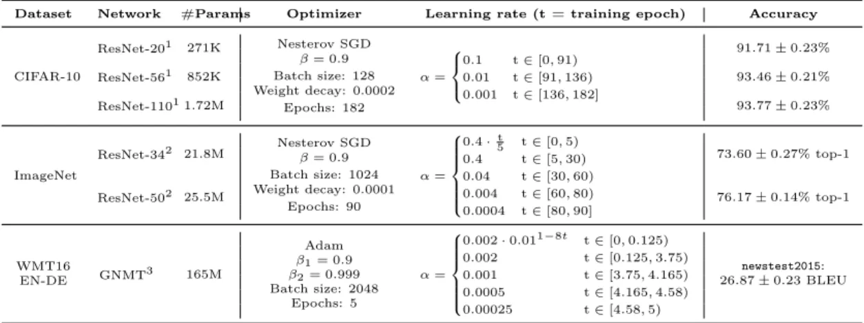
This thesis studies neural network pruning on a variety of standard architectures for image classification and machine translation. These standard networks include ResNet-56 (He et al., 2016) for CIFAR-10 (Krizhevsky, 2009), ResNet-34 and ResNet-50 (He et al., 2016) for ImageNet (Russakovsky et al., 2015), and GNMT (Wu et al., 2016) for WMT16 EN-DE. The implementations and hyperparameters are from standard reference implementations, as described in Table 3.1, with the exception of the GNMT

(19)

model. The GNMT experiments use an extended training schedule longer than the one used in the reference implementation, such that the extended training schedule reaches standard BLEU scores on the validation set, rather than the lower BLEU reached by the reference implementation.1 _{This extended schedule uses the same}

standard GNMT warmup and decay schedule as the original training schedule (Luong et al., 2017), but expanded to span 5 epochs rather than 2.

Dataset Network #Params Optimizer Learning rate (t = training epoch) Test accuracy

CIFAR-10 ResNet-562 _852K Nesterov SGD 𝛽 = 0.9 Batch size: 128 Weight decay: 0.0002 Epochs: 182 𝛼 = ⎧ ⎪ ⎨ ⎪ ⎩ 0.1 t ∈ [0, 91) 0.01 t ∈ [91, 136) 0.001 t ∈ [136, 182] 93.46 ± 0.21% ImageNet ResNet-343 21.8M Nesterov SGD𝛽 = 0.9 Batch size: 1024 Weight decay: 0.0001 Epochs: 90 𝛼 = ⎧ ⎪ ⎪ ⎪ ⎪ ⎪ ⎨ ⎪ ⎪ ⎪ ⎪ ⎪ ⎩ 0.4 ·t₅ t ∈ [0, 5) 0.4 t ∈ [5, 30) 0.04 t ∈ [30, 60) 0.004 t ∈ [60, 80) 0.0004 t ∈ [80, 90] 73.60 ± 0.27% top-1 ResNet-503 25.5M 76.17 ± 0.14% top-1 WMT16 EN-DE GNMT4 165M Adam 𝛽1= 0.9 𝛽2= 0.999 Batch size: 2048 Epochs: 5 𝛼 = ⎧ ⎪ ⎪ ⎪ ⎪ ⎪ ⎨ ⎪ ⎪ ⎪ ⎪ ⎪ ⎩ 0.002 · 0.011−8𝑡 t ∈ [0, 0.125) 0.002 t ∈ [0.125, 3.75) 0.001 t ∈ [3.75, 4.165) 0.0005 t ∈ [4.165, 4.58) 0.00025 t ∈ [4.58, 5) newstest2015: 26.87 ± 0.23 BLEU

Table 3.1: Networks, datasets, and hyperparameters. All networks use standard implementations available online and standard hyperparameters. All accuracies are in line with baselines reported for these networks (Liu et al., 2019; He et al., 2018; Gale et al., 2019; Wu et al., 2016; Zhu & Gupta, 2018).

3.2 _Prune

What structure is pruned?

Unstructured pruning. Unstructured pruning prunes individual weights without consideration for where they occur within each tensor (e.g., Han et al., 2015).

Structured pruning. Structured pruning involves pruning weights in groups, removing neurons, convolutional filters, or channels (e.g., Li et al., 2017).

1_{The reference implementation is from MLPerf 0.5 (Mattson et al., 2020) and reaches a}

newstest-2014 BLEU of 21.8. The extended training schedule reaches a more standard BLEU of 24.2 (Wu et al., 2016). 2 https://github.com/tensorflow/models/tree/v1.13.0/official/resnet 3 https://github.com/tensorflow/tpu/tree/98497e0b/models/official/resnet 4 https://github.com/mlperf/training_results_v0.5/tree/7238ee7/v0.5.0/google/cloud_v3.8/gnmt-tpuv3-8

(20)

Unstructured pruning reduces the number of parameters, but may not improve performance on commodity hardware until a large fraction of weights have been pruned (Park et al., 2017). Structured pruning preserves dense computation, meaning that it can lead to immediate performance improvements (Liu et al., 2017). This thesis studies both unstructured and structured pruning.

What pruning heuristic is used?

Magnitude pruning. Pruning weights with the lowest magnitudes (Han et al., 2015) is a standard choice that achieves state-of-the-art Accuracy versus Efficiency tradeoffs (Gale et al., 2019). For unstructured pruning, the lowest magnitude weights are pruned globally throughout the network (Lee et al., 2019; Frankle & Carbin, 2019). For structured pruning, convolutional filters are pruned by their 𝐿1 norms using the

per-layer pruning rates hand-chosen by Li et al. (2017), specifically, the ResNet-56-B and the ResNet-34-A.5

This thesis only considers magnitude-based pruning heuristics, although there are a wide variety of other pruning heuristics in the literature, including those that learn which weights to prune as part of the optimization process (e.g., Louizos et al., 2018; Molchanov et al., 2017) and those that prune based on other information (e.g., Le Cun et al., 1990; Theis et al., 2018; Lee et al., 2019).

3.3 _Retrain

Let 𝑊𝑔 ∈ R𝑑 be the weights at epoch𝑔. Let 𝑚∈ {0, 1}𝑑 be the pruning mask, such

that the element-wise product 𝑊_{⊙ 𝑚 denotes the pruned network. Let 𝑇 be the} number of epochs that the network is trained for. Let𝑆[𝑔] be the learning rate for each epoch 𝑔, defined such that 𝑆[𝑔 > 𝑇 ] = 𝑆[𝑇 ] (i.e., the last learning rate is extended indefinitely). Let Train𝑡(𝑊, 𝑚, 𝑔) be a function that trains the network 𝑊⊙ 𝑚 for 𝑡 epochs according to the original learning rate schedule𝑆, starting from epoch 𝑔.

5_{To study multiple sparsity levels using these hand-chosen rates, these per-layer pruning rates}

are extrapolated to higher levels of sparsity, by exponentiating each per-layer pruning rate 𝑝𝑖 (which

(21)

Fine-tuning. Fine-tuning retrains the unpruned weights from their final values for a specified number of epochs 𝑡 using a fixed learning rate. Fine-tuning is the current standard practice in the literature (Han et al., 2015; Liu et al., 2019). It is typical to fine-tune using the last learning rate of the original training schedule (Li et al., 2017; Liu et al., 2019), a convention followed in the experiments. Other choices are possible, including those found through hyperparameter search (Han et al., 2015; Han, 2017; Guan et al., 2019). Formally, fine-tuning for _{𝑡 epochs runs Train}𝑡(𝑊𝑇, 𝑚, 𝑇 ).

Weight rewinding. Weight rewinding retrains by rewinding the unpruned weights to their values from 𝑡 epochs earlier in training and subsequently retraining the unpruned weights from there. It also rewinds the learning rate schedule to its state from 𝑡 epochs earlier in training. Retraining with weight rewinding therefore depends on the hyperparameter choices made during the initial training phase of the unpruned network. Weight rewinding was proposed to study the lottery ticket hypothesis by Frankle et al. (2019). Formally, weight rewinding for 𝑡 epochs runs Train𝑡(𝑊𝑇 −𝑡, 𝑚, 𝑇 − 𝑡).

Learning rate rewinding. Learning rate rewinding is a hybrid between fine-tuning and weight rewinding. Like fine-fine-tuning, it uses the final weight values from the end of training. However, when retraining for 𝑡 epochs, learning rate rewinding uses the learning rate schedule from the last 𝑡 epochs of training (what weight rewinding would use) rather than the final learning rate from training (what fine-tuning would use). Formally, learning rate rewinding for _{𝑡 epochs runs Train}𝑡(𝑊𝑇, 𝑚, 𝑇 − 𝑡). I

propose learning rate rewinding in this thesis as a novel retraining technique.

In this thesis, I compare all three retraining techniques. For each network, I consider ten retraining times 𝑡 evenly distributed between 0 epochs and the number of epochs for which the network was originally trained. For iterative pruning, this retraining time is ran per pruning iteration.

(22)

3.4 Iterative pruning

One-shot pruning. The outline above prunes the network to a target sparsity level all at once, known as one-shot pruning (Li et al., 2017; Liu et al., 2019).

Iterative pruning. An alternative is to iterate steps 2 and 3, pruning weights (step 2), retraining (step 3), pruning more weights, retraining further, etc., until a target sparsity level is reached. Doing so is known as iterative pruning. In practice, iterative pruning typically makes it possible to prune more weights while maintaining accuracy (Han et al., 2015; Frankle & Carbin, 2019).

This thesis considers both one-shot and iterative pruning. When running iterative pruning, 20% of weights are pruned per iteration (Frankle & Carbin, 2019). When iteratively pruning with weight rewinding, weights are always rewound to the same values 𝑊𝑇 −𝑡 from the original run of training.

3.5 Metrics

In this thesis, I evaluate a pruned network according to three criteria.

Accuracy is the performance of the pruned network on unseen data from the same distribution as the training set (i.e., the validation or test set). Higher accuracy values indicate better performance, and a typical goal is to match the accuracy of the unpruned network. All plots show the median, minimum, and maximum test accuracies reached across three different training runs.

For vision networks, 20% of the original test set, selected at random, is used as the validation set; the remainder of the original test set is used to report test accuracies. For WMT16 EN-DE, newstest2014 is used as the validation set (following Wu et al., 2016), and newstest2015 is used as the test set (following Zhu & Gupta, 2018).

Efficiency is the resources required to represent or perform inference with the pruned network. This can take multiple forms. This thesis studies Parameter-Efficiency, the parameter count of the network. Parameter-Efficiency is measured relative to the full network with the compression ratio of the pruned network.

(23)

For instance, if the pruned network has 5% of weights remaining, then its compression ratio is 20_{×. Higher compression ratios indicate better Parameter-Efficiency. I} discuss other instantiations of Efficiency in Chapters 7 and 8.

Search Cost is the computational resources required to find the pruning mask and retrain the remaining weights. Search Cost is approximated by retraining time, the total number of additional retraining epochs. Fewer retraining epochs indicates a lower Search Cost. Note that this metric does not consider speedup from retraining pruned networks. For instance, a network pruned to 20_{× compression may be faster} to retrain than if only pruned to 2_{× compression.}

(24)

Chapter 4 Accuracy versus

Parameter-Efficiency tradeoff

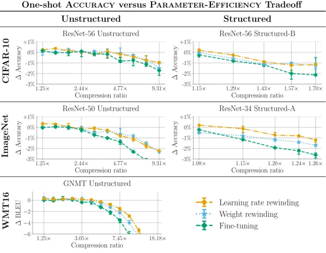
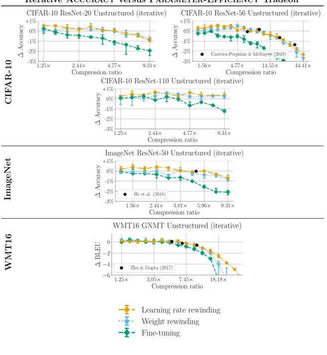
This chapter considers the Pareto frontier of the tradeoff between Accuracy and Parameter-Efficiency using each retraining technique, without regard for Search Cost. In other words, I study the highest accuracy each retraining technique can achieve at each compression ratio. The results show that weight rewinding can achieve higher accuracy than fine-tuning across compression ratios on all studied networks and datasets. Further, learning rate rewinding matches or outperforms weight rewinding in all scenarios. With iterative unstructured pruning, learning rate rewinding achieves state-of-the-art Accuracy versus Parameter-Efficiency tradeoffs, and weight rewinding remains close.

Methodology. For each retraining technique, network, and compression ratio, I select the setting of retraining time with the highest validation accuracy and plot the corresponding test accuracy.

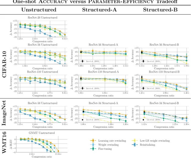
One-shot pruning results. Figure 4-1 presents the results for one-shot pruning. At low compression ratios (when all techniques match the accuracy of the unpruned network), there is little differentiation between the techniques. However, learning rate rewinding typically results in higher accuracy than the unpruned network, whereas other techniques only match the original accuracy. At higher compression ratios (when

(25)

One-shot Accuracy versus Parameter-Efficiency Tradeoff Unstructured Structured CIF AR-10 1.25× 2.44× 4.77× 9.31× Compression ratio -3% -2% -1% 0% +1% ∆ Accuracy ResNet-56 Unstructured 1.15× 1.29× 1.43× 1.57× 1.70× Compression ratio -3% -2% -1% 0% +1% ∆ Accuracy ResNet-56 Structured-B ImageNet 1.25× 2.44× 4.77× 9.31× Compression ratio -3% -2% -1% 0% +1% ∆ Accuracy ResNet-50 Unstructured 1.08× 1.15× 1.20× 1.24× 1.26× Compression ratio -3% -2% -1% 0% +1% ∆ Accuracy ResNet-34 Structured-A WMT16 1.25× 3.05× 7.45× 18.18× Compression ratio −6 −4 −2 0 ∆ BLEU GNMT Unstructured

Learning rate rewinding Weight rewinding Fine-tuning

Figure 4-1: The best achievable accuracy across retraining times by one-shot pruning.

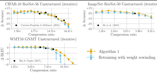
Iterative Accuracy versus Parameter-Efficiency Tradeoff

1.56× 4.77× 14.55× 44.41× Compression ratio -3% -2% -1% 0% +1% ∆ Accuracy

CIFAR-10 ResNet-56 Unstructured (iterative)

1.56× 2.44× 3.81× 5.96× 9.31× Compression ratio -3% -2% -1% 0% +1% ∆ Accuracy

ImageNet ResNet-50 Unstructured (iterative)

1.25× 3.05× 7.45× 18.18× Compression ratio −6 −4 −2 0 ∆ BLEU WMT16 GNMT Unstructured (iterative) Fine-tuning

(26)

no techniques match the unpruned network accuracy), there is more differentiation between the techniques, with fine-tuning losing more accuracy than either rewinding technique. Weight rewinding outperforms fine-tuning in all scenarios. Learning rate rewinding in turn outperforms weight rewinding by a small margin.

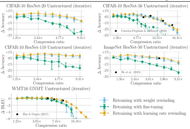
Iterative pruning results. Figure 4-2 presents the results for iterative unstructured pruning. As a basis for comparison, Figure 4-2 also presents the drop in accuracy achieved by state-of-the-art techniques (as described in Section 2.4 and shown to be state-of-the-art by Blalock et al. (2020)) as individual black dots. In iterative pruning, weight rewinding continues to outperform fine-tuning, and learning rate rewinding continues to outperform weight rewinding. Learning rate rewinding matches the Accuracy versus Parameter-Efficiency tradeoffs of state-of-the-art techniques across all datasets. In particular, learning rate rewinding with iterative unstructured pruning produces a ResNet-50 that matches the accuracy of the original network at 5.96× compression, a new state-of-the-art ResNet-50 compression ratio with no drop in accuracy. Weight rewinding nearly matches these state-of-the-art results, with the exception of high compression ratios on GNMT.

Takeaway. Retraining with weight rewinding outperforms retraining with fine-tuning across networks and datasets. Learning rate rewinding in turn matches or outperforms weight rewinding in all scenarios. Combined with iterative unstructured pruning, learning rate rewinding matches the tradeoffs between Accuracy and Parameter-Efficiency achieved by more complex techniques. Weight rewinding nearly matches these state-of-the-art tradeoffs.

(27)

Chapter 5 Accuracy versus Search Cost

tradeoff

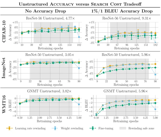
This chapter considers the tradeoff between Accuracy and Search Cost for each retraining technique across a selection of compression ratios. In other words, I study each method’s Accuracy given a fixed Search Cost. The results show that both rewinding techniques achieve higher accuracy than fine-tuning for a variety of different retraining times _{𝑡 (corresponding to different Search Costs). Therefore,} in many contexts either rewinding technique can serve as a drop-in replacement for fine-tuning and achieve higher accuracy. Moreover, the results show that using learning rate rewinding and retraining for the full training time of the original network leads to the highest accuracy among all tested retraining techniques, simplifying the hyperparameter search process.

Methodology. Figures 5-1 (unstructured pruning) and 5-2 (structured pruning) show the accuracy of each retraining technique as the amount of retraining time is varied; that is, the tradeoff between Accuracy and Search Cost. Each plot shows this tradeoff at a specific compression ratio. The left column shows comparisons for No Accuracy Drop, which is defined as the highest compression ratio at which any retraining technique can match the accuracy of the original network for any amount of Search Cost. The right column shows comparisons for 1%/1 BLEU Accuracy Drop,

(28)

Unstructured Accuracy versus Search Cost Tradeoff

No Accuracy Drop 1%/1 BLEU Accuracy Drop

CIF AR-10 10 39 67 96 125 153 182 Retraining epochs -3% -2% -1% 0% +1% ∆ Accuracy ResNet-56 Unstructured, 4.77× 10 39 67 96 125 153 182 Retraining epochs -3% -2% -1% 0% +1% ∆ Accuracy ResNet-56 Unstructured, 9.31× ImageNet 9 22 36 50 63 76 90 Retraining epochs -6% -4% -2% 0% ∆ Accuracy ResNet-50 Unstructured, 3.05× 9 22 36 50 63 76 90 Retraining epochs -6% -4% -2% 0% ∆ Accuracy ResNet-50 Unstructured, 5.96× WMT16 0.50 1.25 2.00 2.75 3.50 4.25 5.00 Retraining epochs −8 −6 −4 −2 0 ∆ BLEU GNMT Unstructured, 3.82× 0.50 1.25 2.00 2.75 3.50 4.25 5.00 Retraining epochs −8 −6 −4 −2 0 ∆ BLEU GNMT Unstructured, 5.96×

Learning rate rewinding Weight rewinding Fine-tuning Rewinding safe zone

Figure 5-1: Accuracy curves across networks and compression ratios using unstructured pruning.

(29)

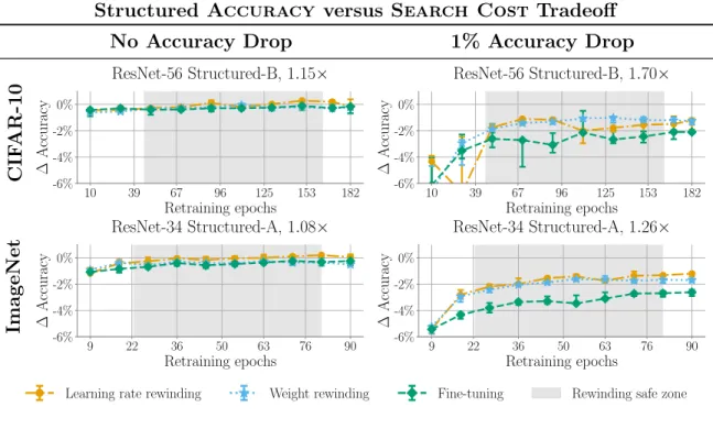
Structured Accuracy versus Search Cost Tradeoff

No Accuracy Drop 1% Accuracy Drop

CIF AR-10 10 39 67 96 125 153 182 Retraining epochs -6% -4% -2% 0% ∆ Accuracy ResNet-56 Structured-B, 1.15× 10 39 67 96 125 153 182 Retraining epochs -6% -4% -2% 0% ∆ Accuracy ResNet-56 Structured-B, 1.70× ImageNet 9 22 36 50 63 76 90 Retraining epochs -6% -4% -2% 0% ∆ Accuracy ResNet-34 Structured-A, 1.08× 9 22 36 50 63 76 90 Retraining epochs -6% -4% -2% 0% ∆ Accuracy ResNet-34 Structured-A, 1.26×

Learning rate rewinding Weight rewinding Fine-tuning Rewinding safe zone

Figure 5-2: Accuracy curves across networks and compression ratios using structured pruning.

which is defined as the highest compression ratio at which any retraining technique gets within 1% accuracy or 1 BLEU of the original network. Similar plots for all tested compression ratios are included in Appendix B. All results presented in this chapter are for one-shot pruning; Appendix B also includes iterative pruning results, which exhibit the same trends.

Unstructured pruning results. Both rewinding techniques almost always match or outperform fine-tuning for equivalent retraining epochs. The sole exception is using weight rewinding and retraining for the full original training time, thereby rewinding the weights to the beginning of training: Frankle et al. (2019) show that accuracy drops if weights are rewound too close to initialization, and the same behavior is found here. To characterize the regions that show good performance for rewinding, I define the rewinding safe zone as the maximal region (as a percentage of original training time) across all networks in which both forms of rewinding outperform fine-tuning for an equivalent Search Cost. This zone (shaded gray in Figure 5-1) occurs when

(30)

retraining for 25% to 90% of the original training time. Within this region, either rewinding technique can serve as a drop-in replacement for fine-tuning.

With learning rate rewinding, retraining for longer almost always results in higher accuracy. The same is true for weight rewinding other than when weights are rewound to near the beginning of training. On most networks and compression ratios, accuracy from rewinding saturates after retraining for roughly half of the original training time: while accuracy can continue to increase with more retraining, this gain is limited. Structured pruning results. Structured pruning exhibits the same trends as unstructured pruning,1 _{except that retraining with weight rewinding does not result}

in a drop in accuracy when retraining for the full training time (thereby rewinding to the beginning of training). This is consistent with the findings of Liu et al. (2019), who show that fine-tuning after structured pruning provides no accuracy advantage over reinitializing and training the pruned network from scratch. Liu et al. (2019) indicate that initialization is less consequential for retraining after structured pruning than for it is for retraining after unstructured pruning. Since weight rewinding and learning rate rewinding only differ in initialization before retraining, both techniques attain similar accuracies when used for retraining after structured pruning.

Takeaway. Both weight rewinding and learning rate rewinding outperform fine-tuning across a wide range of retraining times, thereby serving as drop-in replacements that achieve higher accuracy anywhere within the rewinding safe zone. To achieve the most accurate network, retrain with learning rate rewinding for the full original training time (although accuracy saturates after retraining for about half of the original training time).

1_{On the CIFAR-10 ResNet-56 Structured-B at 1% Accuracy Drop, the experimental results show}

that learning rate rewinding reaches lower accuracy than fine-tuning when retraining for 30 epochs. At this retraining time, the techniques are identical: the learning rate in the last 30 epochs of training, which learning rate rewinding uses, is the same as the final learning rate, which fine-tuning uses. The observed accuracy difference at that point therefore appears to be a result of random noise, and is not characteristic of the retraining techniques.

(31)

Chapter 6 Pruning algorithm based on learning

rate rewinding

Based on the results in Chapters 4 and 5, this chapter proposes a pruning algorithm that is on the state-of-the-art Accuracy versus Parameter-Efficiency Pareto frontier. Algorithm 1 presents an instantiation of the pruning algorithm from Chapter 3 using network-agnostic hyperparameters:

Algorithm 1 SOTA pruning algorithm based on learning rate rewinding 1. Train to completion.

2. Prune the 20% lowest-magnitude weights globally.

3. Retrain using learning rate rewinding for the original training time.

4. Repeat steps 2 and 3 iteratively until the desired compression ratio is reached.

Figure 6-1 presents an evaluation of Algorithm 1. Specifically, Figure 6-1 compares the Accuracy versus Parameter-Efficiency tradeoff achieved by Algorithm 1, by weight rewinding (as in the iterative section of Chapter 4), and by state-of-the-art baselines. This results in the same state-of-the-art behavior seen in Chapter 4, without requiring any per-compression-ratio hyperparameter search. Appendix A presents comparisons of Algorithm 1 instantiated with other retraining techniques.

(32)

Accuracy versus Parameter-Efficiency Tradeoff from Algorithm 1 1.56× 4.77× 14.55× 44.41× Compression ratio -3% -2% -1% 0% +1% ∆ Accuracy

Carreira-Perpi˜n´an & Idelbayev (2018)

He et al. (2018) 1.25× 3.05× 7.45× 18.18× Compression ratio −6 −4 −2 0 ∆ BLEU WMT16 GNMT Unstructured (iterative)

Zhu & Gupta (2017)

Algorithm 1

Retraining with weight rewinding

Figure 6-1: Accuracy versus Parameter-Efficiency tradeoff of Algorithm 1. considered in this thesis: there are neither layer-wise pruning rates nor a pruning schedule to select, beyond the network-agnostic 20% per-iteration pruning rate from prior work (Frankle & Carbin, 2019). Moreover, Algorithm 1 matches the accuracy of pruning algorithms that require more hyperparameters and/or additional methods, such as reinforcement learning (He et al., 2018; Carreira-Perpiñán & Idelbayev, 2018; Zhu & Gupta, 2018).

In all tested networks, the best selection of retraining time for weight rewinding nearly matches the performance of Algorithm 1, with the exception of at high com-pression ratios on the GNMT. This shows that lottery tickets found by pruning and rewinding are state-of-the-art pruned networks.

(33)

Chapter 7 Inference-Efficiency of iteratively

pruned networks

In the chapters above, I use the compression ratio (Parameter-Efficiency) as the metric denoting the Efficiency of a given neural network. However, the compression ratio does not tell the full story: networks of different compression ratios can require different amounts of floating point operations (FLOPs) to perform inference. For instance, pruning a weight in the first convolutional layer of a ResNet results in pruning more FLOPs than pruning a weight in the last convolutional layer, since the input feature maps are larger at the beginning of the network. Reduction in FLOPs can (but does not necessarily) result in wall clock speedup (Baghdadi et al., 2019). In this chapter, I analyze the number of FLOPs required to perform inference on pruned networks acquired through fine-tuning and rewinding. The methodology for one-shot pruning uses the same initial trained network for our comparisons between all techniques, and prunes using the same pruning technique. This means that both networks have the exact same sparsity pattern, and therefore same number of FLOPs. For iterative pruning the networks diverge, meaning the FLOPs also differ, since weights are pruned globally, and can therefore be pruned in different amount from different layers.

(34)

Iterative pruning FLOP speedup over original network 1.56× 2.44× 3.81× 5.96× 9.31× Compression Ratio 2.00× 4.00× 6.00× Sp eedup

ResNet-56 best-validated FLOPs across densities

1.56× 2.44× 3.81× 5.96× 9.31× Compression Ratio 2.00× 4.00× 6.00× Sp eedup

Figure 7-1: Speedup over original network for different retraining techniques and networks

Iterative pruning FLOP speedup over fine-tuning

1.56× 2.44× 3.81× 5.96× 9.31× Compression Ratio 0.90× 1.00× 1.10× 1.20× 1.30× Sp eedup

ResNet-56 speedup of best-validated FLOPs over fine-tuning

Figure 7-2: Speedup over original network for different retraining techniques and networks

(35)

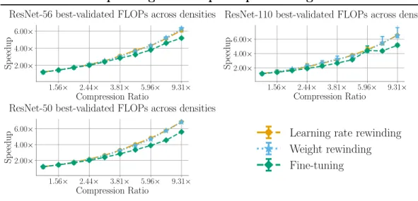
Methodology. In this chapter, I compare the FLOPs of networks resulting from different iteratively applied retraining techniques. I specifically consider iteratively pruned vision networks, where pruning weights in earlier layers results in a larger reduction in FLOPs than pruning weights in later layers. I perform this comparison using the same networks selected in the iterative section of Chapter 4, i.e. using the retraining time that results in the set of networks with the highest validation accuracy for each different compression ratio. Therefore the FLOPs reported in this chapter are the FLOPs resulting from the most accurate network at a given compression ratio, not necessarily the minimum required FLOPs at that compression ratio. Figure 7-1 shows the theoretical speedup over the original network – i.e., the ratio of original FLOPs over pruned FLOPs. Figure 7-2 shows the theoretical speedup of each technique over fine-tuning – i.e., the ratio of fine-tuning FLOPs at that compression ratio to the FLOPs of each other technique at that compression ratio.

Results. Both rewinding techniques discover networks that require fewer FLOPs than those found by iterative pruning with standard fine-tuning. Due to the in-creased accuracy from rewinding, this results in a magnified decrease in Inference-Efficiency for rewinding compared to fine-tuning. For instance, a ResNet-50 pruned to maintain the same accuracy as the original network results in a 4.8× theoreti-cal speedup from the original network when rewinding the learning rate, whereas a similarly accurate network attained through fine-tuning has a speedup of 1.7×.

(36)

Chapter 8 Discussion

Weight rewinding. When retraining with weight rewinding, the weights are re-wound to their values from early in training. This means that after retraining with weight rewinding, the weights themselves receive no more gradient updates than in the original training phase. Nevertheless, weight rewinding outperforms fine-tuning and is competitive with learning rate rewinding, losing little accuracy even though it reverts most of training. These results show that when pruning, it is not necessary to train the weights for a large number of steps; the pruning mask itself is a valuable output of pruning.

Learning rate rewinding. This thesis proposes learning rate rewinding, an alterna-tive retraining technique that achieves state-of-the-art Accuracy versus Parameter-Efficiency tradeoffs. This thesis does not investigate why the learning rate schedule used by learning rate rewinding achieves higher accuracy than that of the standard fine-tuning schedule. I hope that further work on the optimization of sparse neural networks can shed light on why learning rate rewinding achieves higher accuracy than standard fine-tuning and can help derive other techniques for the training of sparse networks (Smith, 2017; Dettmers & Zettlemoyer, 2019).

The retraining techniques considered reuse the hyperparameters from the origi-nal training process. This choice inherently narrows the design space of retraining techniques by coupling the learning rate schedule of retraining to that of the original

(37)

training process. There may be further opportunities to improve performance by decoupling the hyperparameters of training and retraining and considering other retraining learning rate schedules. However, these potential opportunities come with the cost of added hyperparameter search.

Search Cost. Achieving state-of-the-art Accuracy versus Parameter-Efficiency tradeoffs with Algorithm 1 requires substantial Search Cost. Algorithm 1 requires 𝑇 _{· (1 + 𝑘) total training epochs to reach compression ratio 1 / 0.8}𝑘_{, where}_{𝑇 is the}

original network training time, and 𝑘 is the number of pruning iterations. In contrast, on CIFAR-10 (𝑇 = 182 epochs) Carreira-Perpiñán & Idelbayev (2018) employ a grad-ual pruning technique followed by fine-tuning, training for a total of 317 epochs to reach any compression ratio. On ImageNet (𝑇 = 90 epochs), He et al. (2018) retrain the ResNet-50 for 376 epochs to match the accuracy of the original network at 5.13× compression. On WMT-16 (𝑇 = 5 epochs), Zhu & Gupta (2018) use a gradual pruning technique that trains and prunes over the course of about 11 epochs to reach any compression ratio.

The Search Costs of these other methods do not take into account the per-network hyperparameter search that each method required to find the settings that produced the reported results, nor the cost of the pruning heuristics themselves (e.g., training a reinforcement learning agent to predict pruning rates). In addition to optimizing the tradeoff between Accuracy and Parameter-Efficiency, future pruning research should also consider Search Cost (including hyperparameter search and training time).

Efficiency. This thesis studies Parameter-Efficiency: the number of pa-rameters in the network. This provides a notion of scale of the network (Rosenfeld et al., 2020) and can serve as an input for theoretical analyses (Arora et al., 2018). There are other useful forms of Efficiency that are not studied in this thesis. One commonly studied form is Inference-Efficiency, the cost of performing infer-ence with the pruned network. This is often measured in floating point operations (FLOPs) or wall clock time (Han, 2017; Han et al., 2016a). In Chapters 4 and 5, I

(38)

demonstrate that both rewinding techniques outperform fine-tuning after structured pruning (which explicitly targets Inference-Efficiency). In Chapter 7, I show that iterative unstructured pruning and retraining with either rewinding technique results in networks that require fewer FLOPs to execute than those found by iterative unstructured pruning and retraining with fine-tuning.

Other forms of Efficiency that are not studied in this include Storage-Efficiency (Han et al., 2016b), Communication-Storage-Efficiency (Alistarh et al., 2017), and Energy-Efficiency (Yang et al., 2017).

The Lottery Ticket Hypothesis. Weight rewinding was first proposed by work on the lottery ticket hypothesis (Frankle & Carbin, 2019; Frankle et al., 2019), which studies the existence of sparse subnetworks that can train in isolation to full accuracy from near initialization. In this thesis, I present the first detailed comparison between the performance of these lottery ticket networks and pruned networks generated by standard fine-tuning. From this perspective, my results show that the sparse, lottery ticket networks that Frankle et al. (2019) uncover from early in training using weight rewinding can train to full accuracy at compression ratios that are competitive for pruned networks in general.

(39)

Chapter 9 Conclusion

This thesis compares rewinding and fine-tuning as retraining techniques after neural network pruning, investigating the hypothesis that rewinding is a key technique for attaining accurate pruned neural networks. My results show that both weight rewinding and learning rate rewinding can attain higher accuracy than fine-tuning when given equal retraining budgets, and further that the rewinding techniques are not strongly sensitive to hyperparameter choice, attaining higher accuracy than fine-tuning across a wide range of hyperparameters. The analysis of weight rewinding shows that with a proper choice of where to rewind to, lottery tickets found by pruning and rewinding are state-of-the-art pruned networks. Further, with iterative unstructured pruning, learning rate rewinding to the beginning of training matches the Accuracy versus Parameter-Efficiency tradeoffs of more complex techniques requiring network-specific hyperparameters. These results demonstrate that learning rate rewinding is a valuable baseline for future research and a compelling default choice for pruning in practice.

(40)

Bibliography

Dan Alistarh, Demjan Grubic, Jerry Li, Ryota Tomioka, and Milan Vojnovic. QSGD: Communication-efficient sgd via gradient quantization and encoding. In Conference on Neural Information Processing Systems, 2017.

Sanjeev Arora, Rong Ge, Behnam Neyshabur, and Yi Zhang. Stronger generalization bounds for deep nets via a compression approach. In International Conference on Machine Learning, 2018.

Riyadh Baghdadi, Abdelkader Nadir Debbagh, Kamel Abdous, Benhamida Fatima Zohra, Alex Renda, Jonathan Frankle, Michael Carbin, and Saman Amarasinghe. Tiramisu: A polyhedral compiler for dense and sparse deep learning. In SysML Workshop, Conference on Neural Information Processing Systems, 2019.

Davis Blalock, Jose Javier Gonzalez Ortiz, Jonathan Frankle, and John Guttag. What is the state of neural network pruning? In Conference on Machine Learning and Systems, 2020.

Miguel Á Carreira-Perpiñán and Yerlan Idelbayev. “Learning-Compression” algorithms for neural net pruning. In IEEE/CVF Conference on Computer Vision and Pattern Recognition, 2018.

Tim Dettmers and Luke Zettlemoyer. Sparse networks from scratch: Faster training without losing performance, arXiv preprint arXiv:1907.04840, 2019.

(41)

trainable neural networks. In International Conference on Learning Representations, 2019.

Jonathan Frankle, Gintare Karolina Dziugaite, Daniel M. Roy, and Michael Carbin. Linear mode connectivity and the lottery ticket hypothesis, arXiv preprint arXiv:1912.05671, 2019.

Trevor Gale, Erich Elsen, and Sara Hooker. The state of sparsity in deep neural networks, arXiv preprint arXiv:1902.09574, 2019.

Hui Guan, Xipeng Shen, and Seung-Hwan Lim. Wootz: A compiler-based frame-work for fast cnn pruning via composability. In ACM SIGPLAN Conference on Programming Language Design and Implementation, 2019.

Song Han. Efficient Methods and Hardware for Deep Learning. PhD thesis, Stanford University, 2017.

Song Han, Jeff Pool, John Tran, and William Dally. Learning both weights and connections for efficient neural network. In Conference on Neural Information Processing Systems. 2015.

Song Han, Xingyu Liu, Huizi Mao, Jing Pu, Ardavan Pedram, Mark A. Horowitz, and William J. Dally. Eie: Efficient inference engine on compressed deep neural network. In International Symposium on Computer Architecture, 2016a.

Song Han, Huizi Mao, and William J. Dally. Deep compression: Compressing deep neu-ral network with pruning, trained quantization and huffman coding. In International Conference on Learning Representations, 2016b.

Babak Hassibi, David G. Stork, Gregory Wolff, and Takahiro Watanabe. Optimal brain surgeon: Extensions and performance comparisons. In Conference on Neural Information Processing Systems, 1993.

Kaiming He, Xiangyu Zhang, Shaoqing Ren, and Jian Sun. Deep residual learning for image recognition. In IEEE/CVF Conference on Computer Vision and Pattern Recognition, 2016.

(42)

Yihui He, Ji Lin, Zhijian Liu, Hanrui Wang, Li-Jia Li, and Song Han. AMC: Automl for model compression and acceleration on mobile devices. In European Conference on Computer Vision, 2018.

John Hertz, Anders Krogh, and Richard G. Palmer. Introduction to the Theory of Neural Computation. Addison-Wesley Longman Publishing Co., Inc., USA, 1991. Alex Krizhevsky. Learning multiple layers of features from tiny images. Technical

report, 2009.

Yann Le Cun, John S. Denker, and Sara A. Solla. Optimal brain damage. In Conference on Neural Information Processing Systems, 1990.

Namhoon Lee, Thalaiyasingam Ajanthan, and Philip Torr. SNIP: Single-shot network pruning bassed on connection sensitivity. In International Conference on Learning Representations, 2019.

Hao Li, Asim Kadav, Igor Durdanovic, Hanan Samet, and Hans Peter Graf. Pruning filters for efficient convnets. In International Conference on Learning Representations, 2017.

Zhuang Liu, Jianguo Li, Zhiqiang Shen, Gao Huang, Shoumeng Yan, and Changshui Zhang. Learning efficient convolutional networks through network slimming. In International Conference on Computer Vision, 2017.

Zhuang Liu, Mingjie Sun, Tinghui Zhou, Gao Huang, and Trevor Darrell. Rethinking the value of network pruning. In International Conference on Learning Representa-tions, 2019.

Christos Louizos, Max Welling, and Diederik P. Kingma. Learning sparse neural networks through l0 regularization. In International Conference on Learning Repre-sentations, 2018.

Minh-Thang Luong, Eugene Brevdo, and Rui Zhao. Neural machine translation (seq2seq) tutorial. https://github.com/tensorflow/nmt, 2017.

(43)

Peter Mattson, Christine Cheng, Cody Coleman, Greg Diamos, Paulius Micikevicius, David Patterson, Hanlin Tang, Gu-Yeon Wei, Peter Bailis, Victor Bittorf, David Brooks, Dehao Chen, Debojyoti Dutta, Udit Gupta, Kim Hazelwood, Andrew Hock, Xinyuan Huang, Bill Jia, Daniel Kang, David Kanter, Naveen Kumar, Jeffery Liao, Guokai Ma, Deepak Narayanan, Tayo Oguntebi, Gennady Pekhimenko, Lillian Pentecost, Vijay Janapa Reddi, Taylor Robie, Tom St. John, Carole-Jean Wu, Lingjie Xu, Cliff Young, and Matei Zaharia. Mlperf training benchmark. In Conference on Machine Learning and Systems, 2020.

Dmitry Molchanov, Arsenii Ashukha, and Dmitry Vetrov. Variational dropout sparsifies deep neural networks. In International Conference on Machine Learning, 2017. Jongsoo Park, Sheng Li, Wei Wen, Ping Tak Peter Tang, Hai Li, Yiran Chen, and

Pradeep Dubey. Faster cnns with direct sparse convolutions and guided pruning. In International Conference on Learning Representations, 2017.

Russell Reed. Pruning algorithms–a survey. IEEE Transactions on Neural Networks, 1993.

Alex Renda, Jonathan Frankle, and Michael Carbin. Comparing rewinding and fine-tuning in neural network pruning. In International Conference on Learning Representations, 2020.

Jonathan S. Rosenfeld, Amir Rosenfeld, Yonatan Belinkov, and Nir Shavit. A construc-tive prediction of the generalization error across scales. In International Conference on Learning Representations, 2020.

Olga Russakovsky, Jia Deng, Hao Su, Jonathan Krause, Sanjeev Satheesh, Sean Ma, Zhiheng Huang, Andrej Karpathy, Aditya Khosla, Michael Bernstein, Alexan-der C. Berg, and Li Fei-Fei. ImageNet Large Scale Visual Recognition Challenge. International Journal of Computer Vision, 2015.

Jocelyn Sietsma and Robert J.F. Dow. Creating artificial neural networks that generalize. Neural Networks, 1991.

(44)

Sietsma, Jocelyn and Dow, Robert J.F. Neural net pruning-why and how. In IEEE International Conference on Neural Networks, 1988.

Leslie N. Smith. Cyclical learning rates for training neural networks. IEEE Winter Conference on Applications of Computer Vision, 2017.

Lucas Theis, Iryna Korshunova, Alykhan Tejani, and Ferenc Huszár. Faster gaze prediction with dense networks and fisher pruning, arXiv preprint arXiv:1801.05787, 2018.

Yonghui Wu, Mike Schuster, Zhifeng Chen, Quoc V. Le, Mohammad Norouzi, Wolfgang Macherey, Maxim Krikun, Yuan Cao, Qin Gao, Klaus Macherey, Jeff Klingner, Apurva Shah, Melvin Johnson, Xiaobing Liu, Łukasz Kaiser, Stephan Gouws, Yoshikiyo Kato, Taku Kudo, Hideto Kazawa, Keith Stevens, George Kurian, Nishant Patil, Wei Wang, Cliff Young, Jason Smith, Jason Riesa, Alex Rudnick, Oriol Vinyals, Greg Corrado, Macduff Hughes, and Jeffrey Dean. Google’s neural machine translation system: Bridging the gap between human and machine translation, arXiv preprint arXiv:1609.08144, 2016.

Tien-Ju Yang, Yu-Hsin Chen, and Vivienne Sze. Designing energy-efficient convo-lutional neural networks using energy-aware pruning. In IEEE Conference on Computer Vision and Pattern Recognition, 2017.

Michael Zhu and Suyog Gupta. To prune, or not to prune: Exploring the efficacy of pruning for model compression. In International Conference on Learning Represen-tations Workshop Track, 2018.

Barret Zoph and Quoc V. Le. Neural architecture search with reinforcement learning. In International Conference on Learning Representations, 2017.

(45)

Appendix Table of Contents

Appendix A evaluates Chapter 6 instantiated with other retraining methods than learning rate rewinding.

Appendix B extends the results in the main body of the thesis to include more networks, pruning techniques, baselines, and ablations.

(46)

Appendix A

Other instantiations of Algorithm 1

In this appendix, I present a comparison of the algorithm presented in Chapter 6 to instantiations of that algorithm with other retraining techniques. Specifically, I compare against retraining with weight rewinding for 90% of the original training time, learning rate rewinding for the original training time (as presented in the algorithm in the main body of the paper), or fine-tuning for the original training time.

Algorithm 2 SOTA pruning algorithm 1. Train to completion.

2. Prune the 20% lowest-magnitude weights globally.

3. Retrain using either weight rewinding for 90% of the original training time, learning rate rewinding for the original training time, or fine-tuning for the original training time.

4. Repeat steps 2 and 3 iteratively until the desired compression ratio is reached.

Figure A-1 presents an evaluation of Algorithm 2. The results show that retraining with weight rewinding performs similarly well to retraining with learning rate rewinding, except for at high sparsities on the GNMT.

(47)

Accuracy versus Parameter-Efficiency Tradeoff from Algorithm 2 1.25× 2.44× 4.77× 9.31× Compression ratio -3% -2% -1% 0% +1% ∆ Accuracy

Carreira-Perpi˜n´an & Idelbayev (2018)

He et al. (2018) 1.25× 3.05× 7.45× 18.18× Compression ratio −6 −4 −2 0 ∆ BLEU WMT16 GNMT Unstructured (iterative)

Zhu & Gupta (2017)

Retraining with weight rewinding Retraining with fine-tuning

Retraining with learning rate rewinding

(48)

Appendix B

Additional Networks and Baselines

This appendix includes results for more networks, pruning techniques, baselines, and ablations. It considers a larger set of networks than the main body of the thesis, more structured pruning techniques from Li et al. (2017), a reinitialization baseline from Liu et al. (2019), and a natural ablation of rewinding, which rewinds the weights but uses the learning rate of fine-tuning.

Methodology

Retraining techniques. This appendix includes two baselines of the techniques presented in the main body of the thesis, using the notation from Chapter 3. For convenience, that notation is duplicated here.

Neural network pruning is an algorithm that begins with a randomly initialized neural network with weights𝑊0 ∈ R𝑑 and returns two objects: weights𝑊 ∈ R𝑑 and a

pruning mask𝑚 ∈ {0, 1}𝑑 _{such that} _𝑊_{⊙ 𝑚 is the state of the pruned network (where}

⊙ is the element-wise product operator). Let 𝑊𝑔 be the weights of the network at

epoch 𝑔. Let 𝑇 be the standard number of epochs for which the network is trained. Let 𝑆[𝑔] be the learning rate schedule of the network for each epoch 𝑔, defined such that 𝑆[𝑔 > 𝑇 ] = 𝑆[𝑇 ] (i.e., the last learning rate is extended indefinitely). Let Train𝑡(𝑊, 𝑚, 𝑔) be a function that trains the weights of 𝑊 that are not pruned by

(49)

mask 𝑚 for 𝑡 epochs according to the original learning rate schedule 𝑆, starting from step 𝑔.

Low-LR weight rewinding. The other natural ablation of weight rewinding (other than learning rate rewinding) is to rewind just the weights and use the learning rate that would have been used in fine-tuning. Formally, Low-LR weight rewinding for _{𝑡 epochs runs Train}𝑡(𝑊𝑇 −𝑡, 𝑚, 𝑇 ).

Reinitialization. This appendix also includes a baseline of reinitializing the discovered pruned network and retraining it by extending the original training schedule to the same total number of training epochs as fine-tuning trains for. Liu et al. (2019) found that for many pruning techniques, pruning and fine-tuning results in the same or worse performance as simply training the pruned network from scratch for an equivalent number of epochs. To address these concerns, this appendix includes comparisons against random reinitializations of networks with the discovered pruned structure, trained for the original 𝑇 training epochs plus the extra 𝑡 epochs that networks were retrained for. Formally reinitializing and retraining for 𝑡 epochs is sampling a new 𝑊′

0 ∈ R𝑑 then running Train

𝑇 +𝑡_(𝑊′

0, 𝑚, 0).

This reinitialization baseline uses the discovered structure from training and pruning the original network according to the given pruning technique. For unstructured pruning, this discovered structure is the specific structure left behind after magnitude pruning; for structured pruning, this discovered structure is the structure determined by the layerwise rates derived in Li et al. (2017). It is worth noting that in both of these cases, the resulting structure is determined by having trained the network, whether that occurs explicitly (as with unstructured pruning) or implicitly (as Li et al. determine layerwise pruning rates by pruning individual layers of a trained network). One should therefore expect this to perform at least as well as randomly pruning the network before any amount of training, since the pruned structure incorporates knowledge from having already trained the network at least once.

Networks, Datasets, and Hyperparameters. This appendix includes two more CIFAR-10 vision networks in this appendix: ResNet-20 and ResNet-110. It also