Working Papers
Sloan 3714
CISR 272
IFSRC 286-94
IPC 94-005
Computers and Economic Growth:
Firm-Leyel Evidence
Erik Brynjolfsson LQrin Hitt MIT $loan School Cambridge, Massachusetts
First Draft: November, 1993 Current version: August, 1994
Authors' Address: MIT room E53-313 Cambridge, MA 02139
tel: 617-253-4319 email: [email protected]
or lhitt@ sloan.mit.edu
We are grateful to Martin Neil Baily, Rajiv Banker, Ernst Berndt, Tim Bresnahan, Zvi Griliches, Dale Jorgenson, Bronwyn Hall, Rebecca Henderson, Julio Rotemberg, Kevin Stiroh, Robert Solow and
seminar participants at Boston University, Harvard Business School, MIT, the NBER Productivity Workshop, National Technical University in Singapore, the National Science Foundation IT and
Productivity Workshop, Stanford and the U.S. Federal Reserve for valuable comments. This research has been generously supported by the MIT Center for Coordination Science, the MIT Industrial Performance Center, and the MIT International Financial Services Research Center. We would like to
thank Michael Sullivan-Trainor and International Data Group for providing essential data. We alone are responsible for any remaining errors in the paper.
Firm-Level Evidence
ABSTRACT
In advanced economies, computers are a promising source of output growth. This paper assesses the value added by computer equipment and information systems labor by estimating several production
functions that also include ordinary capital, ordinary labor and R&D capital. Our study employs recent firm-level data for 367 large firms which generated approximately $1.8 trillion dollars in output per year for the period 1988 to 1992.
We find evidence that computers are correlated with significantly higher output at the firm level,
although simultaneity makes it difficult to prove a causal relationship. Considering the rapid growth of computer capital stock, our estimates imply that computers were associated with more output growth in the sample period than all other types of capital combined, despite the fact that they accounted for less than 2% of the total capital stock.
I. INTRODUCTION
Historically, estimates of aggregate production functions have suggested that an important determinant of long run economic growth is technical change (Griliches, 1988; Solow, 1957). Technical change is often assumed to be a disembodied function of the passage of time, or modeled as a function of
investments in research and development (R&D). However, Bahk and Gort (1993) provide some evidence that "industry-wide increases in the stock of knowledge [affect] output only insofar as the increases are uniquely related to embodied technical change of physical capital." Furthermore, when advances in knowledge are manifested in "general purpose technologies", dramatically new production possibilities can be created as improvements in complementary technologies magnify even relatively small investments (Bresnahan and Trajtenberg, 1991). The electric dynamo may have played such a role in American manufacturing at the turn of the century (David, 1989). If we now live in the
"information age", it is largely because the computer is increasingly ubiquitous in American offices and factories. The programmable computer is certainly a general purpose technology and the large declines in the costs of computer power reflect substantial research expenditures, as well as some favorable laws of nature. Is the computer the modem economy's engine of growth?
Surprisingly, while anecdotal evidence abounds for the computer-driven successes of specific firms, there has been relatively little econometric evidence that computer technology has added much to economic growth overall (Brynjolfsson, 1993). In part, this is because empirical studies of growth simply have not focused on the role of embodied technical change (Berndt, 1991).1 However, the majority of studies of computers and productivity that have been published have turned up little evidence of positive impact (e.g. (Berndt and Morrison, 1994, in press; Loveman, 1994; Weill,
1992)). After comparing stagnant aggregate productivity growth with the explosion of spending on computers, Robert Solow quipped, "we see computers everywhere but in the productivity statistics" (David, 1989).
It may be possible to unravel this "productivity paradox" by looking at more disaggregate and more current data than were previously available. Our study employs a new data set on 367 large US firms with average annual sales of nearly two trillion dollars over the 1988-1992 time period. We find that investments in computers not only make a statistically significant contribution to output, but they also appear to be associated with significant excess returns. Because real computer capital stock is rapidly increasing, these estimates imply that computers are associated with a contribution of about 1% per year to economic growth for our sample of firms. This contribution is greater than that of all other
capital and several times the contribution of R&D. While there are a number of limitations to this
analysis, it is consistent with the hypothesis that computers are an economically-important embodiment of technical change.
The remainder of the paper is organized as follows. Section II provides some background on
computer technology, discusses the measurement problems inherent in growth accounting, and briefly reviews the findings of other studies which have looked at computers' contributions. Section III discusses the theoretical framework we employ in estimating the production functions, the data used, and the assumptions which underlie our hypothesis tests. The regression results are presented in Section IV and growth accounting calculations are in Section V. We conclude with some possible interpretations of our results in Section VI.
II. BACKGROUND A. Trends in Computing
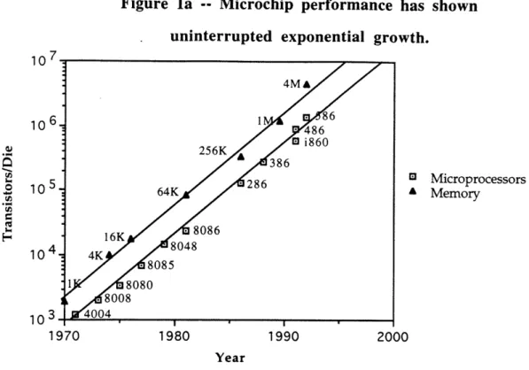
Chip makers have been able to reduce the size of the lines that form transistor circuits by about 10% a year, leading to a doubling of microprocessor power every 18 months. As shown in figure la, these improvement have occurred with such consistency that the trend is generally known in the computer industry as "Moore's Law", after an observation of Gordon Moore, the founder of Intel Corp., in 1964. Furthermore, according to Richard Hollingsworth, the
manager of advanced semiconductor development at Digital Equipment Corporation, nothing is likely to slow this trend in the foreseeable future.
Of course, computers consist of more than just microprocessors. The U.S. Department of Commerce calculates a price of computers which accounts for advances in other components such as random access memory and disk storage and reports that the overall real price of computing power has declined by nearly 20% per year (figure lb), while hedonic estimates by Berndt and Griliches (1990) put the
rate at closer to 25% per year for microcomputers. Software is traditionally viewed as a bottleneck to harnessing the power of computer hardware, although there is some evidence that even here, quality-adjusted prices have declined significantly (Gandal, 1994).
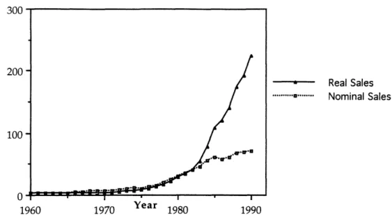
Both nominal and real spending on computers have increased steadily over time (figure 2). The increased spending has been modeled as both a response to lower prices and a function of the gradual diffusion of a superior technology (Gurbaxani and Mendelson, 1990). Despite the rapid growth in computer investment, other capital stock still dwarfs computer stock in dollar terms. In our sample of firms, computers accounted for only about 1.5% of total capital stock.
Computers and Growth: Firm-level Evidence
B. The Mismeasurement Miasma
If these advances in the underlying "technology" of production imply an outward shift of the
production possibility frontier of the economy, the magnitude of this shift has been difficult to assess. The outputs of many firms, especially in the service sector, have never been measured well (Baily and Gordon, 1988). Output measurement is most difficult when new products are created and when existing products are changed qualitatively.
Mismeasurement not only blurs the precision of productivity estimates, it can also lead to systematic biases. In particular, because the benefits of computers are likely to be disproportionately weighted toward outputs that are poorly captured by traditional measures, unsurprisingly, using traditional measures will lead to underestimates of the contribution of computers. For instance, important sources of competitive advantage from computerization include increased product differentiation and improved convenience, not just lower costs (Banker and Kauffman, 1988; Porter and Miller, 1985) .
Furthermore, when managers are asked to rank the benefits of investments in computers, they allocate more weight to improved quality, to customer service, to product variety, and to infrastructure
(creating options for future investment) than to efficiency (Lee, 1993). Each of these benefits is likely to go unmeasured in official price deflators. The true magnitude of the unmeasured benefits is, of course, difficult to quantify, but if the actual benefits of information technologies are proportional to the perceived benefits, then it seems likely that they will be underrepresented when using traditional output measures and deflators.
The use of firm-level data can help mitigate many of the measurement difficulties, although it may exacerbate other problems. To the extent that a firm can appropriate the benefits of improved quality, superior customer service, or better customization by charging higher prices, its sales, value-added, and profits will be increased. However, because benefits that cannot be specifically identified are generally presumed by default not to exist, deflators at the level of the economy as a whole, or for industry aggregates, will attribute such price increases to inflation, and not increased "output". If the higher prices are entirely attributed to inflation, then real output and measured productivity at the industry-level will show no improvement, washing out the different prices commanded by different firms. Firm-level production functions, on the other hand, may better reflect the "true" outputs of the firm, or at least those perceived by its customers, because differences in margins will affect value-added at the firm-level.
On the other hand, firms do not always appropriate the full benefits of their investments. As many managers have lamented, new technology may only "raise the bar", not create lasting competitive advantage (Clemons, 1991). Instead, downstream industries and consumers receive at least some of
the surplus from quality improvements. When the new technology reduces the costs of production, and demand is not elastic, revenues will decrease in a competitive industry.2 Even production
functions estimated with firm-level data will not necessarily discern such benefits unless accurate deflators are available. This dilemma led Bresnahan (1986) to eschew output measures altogether. Instead, he inferred that the benefits of computerization to the financial industry were over an order of magnitude larger than expenditures based on the derived demand for computers. Similarly, based on the rapid quality-adjusted output growth in the computer-producing sector, Mairesse & Hall (1994) estimate that advances in computers account for the majority of the benefits from R&D in the 1980s. However, such analyses cannot tell us whether firms are actually fulfilling the promise of all these computers, since they start with the assumption that their purchasing decisions are optimal.
C. Some of the Previous Research
Work on the sources of growth historically focused on the ways in which technical change affects multifactor productivity (MFP). As noted by Berndt (1991), the vast majority of this research has simply inserted a linear or quadratic time trend variable into production or cost functions, implicitly assuming that MFP is disembodied and proceeds lockstep with the passage of time. A related stream has examined the contributions of R&D "knowledge capital" to growth (e.g. Griliches, 1988; Hall,
1993). Of course, advances in knowledge, per se, will only increase output to the extent they are implemented. While there has been some work making use of patent citation counts as one gauge of the impacts of R&D (e.g. (Jaffe et al., 1993)), a more direct indicator is the extent to which new techniques are embodied in new investment. However, there has been relatively little work examining the role of technical progress embodied in physical capital. One of the most notable exceptions is the growing literature regarding the contribution of information technology (IT) to output and growth. The magnitude and even existence of IT's contribution to growth remains unsettled: several researchers have found low returns to IT, while others have found very high returns.3 Loveman
(1994) estimates a Cobb-Douglas production function for a sample of business units (divisions of firms) for the period 1978-1982 and finds that the gross contribution of computer capital could not be distinguished from zero. Low returns to IT are also found in a series of studies by Berndt, Morrison and Rosenblum, using industry-level data. Estimates of a generalized Leontief cost function using these data suggest that each dollar of IT capital contributed only 80 cents of value on the margin (Morrison and Berndt, 1990). Less highly-parameterized examinations of these data also indicate that
2 Jensen (1993) argues that such technical change characterized many industries in the 1980's, constituting a "modern industrial revolution".
Computers and Growth: Firm-level Evidence
IT capital is on balance not labor-saving, and that overall returns to IT are not significantly different from the returns to other types of capital (Berndt and Morrison, 1994, in press; Berndt et al., 1992). On the other hand, Lau and Tokutsu (1992) find very high returns to IT when they fit a translog production function to time series data for the aggregate U.S. economy. Siegel and Griliches (1991)
find a positive correlation between levels of IT usage and multifactor productivity growth in industry data. Although, after auditing some of the data, they also express serious misgivings about the reliability of government figures and the consistency of industry classifications.
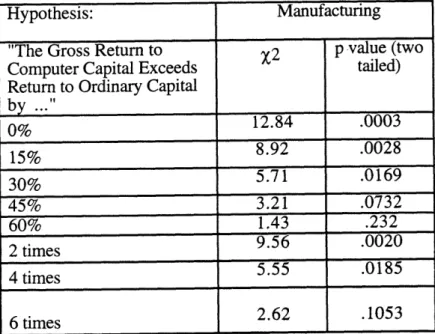
Recently, International Data Group (IDG) has made available firm-level data on several components of information systems spending. Like the industry-level data, these data are subject to limitations and quality concerns, but provide a different perspective on the output contributions of IT. We are aware of two recent studies which examine these data (Brynjolfsson & Hitt, 1993; Lichtenberg, 1993). Brynjolfsson & Hitt (1993) present evidence that the returns to computers may be very high for a broad cross-section of firms. They estimate the output elasticity to be .5% for computers and 1.5% for IS labor which, when compared to their respective factor shares, implies supranormal rates of return for each of these inputs. Lichtenberg (1993) uses a slightly different specification for the production function which confirms these basic findings, and he extends the work in two important ways. First, he finds that computer capital and information system labor also have high returns when data are employed from a different source, Infoweek. Second, he reports that the gross return to computer capital investments exceed the gross return to other capital by over a factor of six, which he argues is the appropriate threshold for hypothesis tests of the equality of net returns, given the higher cost of capital of computers.
On balance, the literature on the contributions of computers to productivity is mixed. However, the new data from IDG present a promising opportunity to obtain more precise estimates of the growth contributions of not only computers, but also other factors of production such as R&D and any residual time trend. While our study is most closely related to the studies of Brynjolfsson and Hitt (1993) and Lichtenberg (1993), it also differs in several important respects. Unlike the other studies, we seek to address concerns of endogeneity by using value-added instead of gross sales as the dependent variable, by instrumenting the independent variables, and by employing a firm effects specification. Second, the use of the firm effects specification and the inclusion of R&D as a distinct input should help to address potential missing variables bias. Third, as a robustness check on our findings, we examine the correlation of computers and R&D with the Solow residual in our sample. Fourth, we use our results to calculate the impact of computers on output growth in two ways. Finally, we present an explanation for the high returns implied by our estimates based on the role of
complementarities between technology, organizations and management policies.
II. MODEL AND DATA
A. Theoretical Framework
To assess the contribution of information technology to output, we begin by positing a production function that relates firm (i) output, Qi,t, to five inputs: computer capital, Ci,t; ordinary capital, Ki,t; information systems labor, Si,t; ordinary labor, Li,t; and materials, Mi,t. We further assume that the production technology can vary over time (t) and across industries (j) yielding:
Qi,t = Q(Ci,,Ki,t,Si,t,LitMi;j t)
One of two alternative special cases is usually assumed in empirical work, depending on whether real sales or value-added is the dependent variable. It is also common to assume separability of the contributions of input factors and the effects of industry and time. For our purposes, these special cases can be written as follows:
Qi't = = A(j,t) F(C;it,Kit,Si, Li,, Mi,t)
Vi, = Qt - Mi, = B(j,t) G(Ci,t,Ki,t,Si,, Lit)
A standard growth accounting framework based on the Solow (1957) model4 assumes that the underlying technology can be approximated by a Cobb-Douglas function, which yields the following estimating equations:
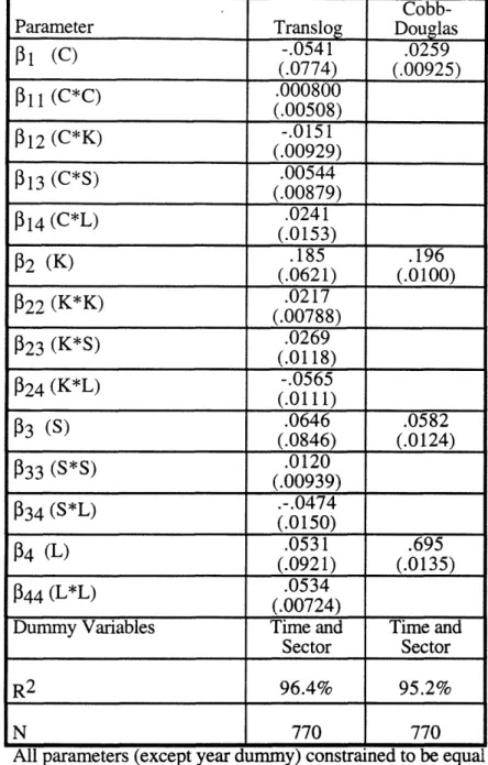
4 See, for example, (Bahk and Gort, 1993; Hall, 1993). While this specification implies some strong assumptions, we also estimated less restrictive translog formulation, using the following equation:
log V = Z (iJ + r T, + p, log X, + Z rlog X, log X
j t-i r s
where: j-industries, Jj are firm dummy variables, t-time, Tt-time dummy variables, Xs are inputs and r,s are index variables on inputs.
The CES production function is a special case of the translog with the additional restriction:
3pS = JPr (for each input s)
We found that the point estimates of the results were not sensitive to the choice of functional form (table 5), although the standard errors were generally higher, owing to multicollinearity and the additional parameters that needed to be estimated. This accords with the Griliches' (1979) suggestion that the Cobb-Douglas form is suitable for the calculation of output elasticities.
Computers and Growth: Firm-level Evidence
Qi., = SJj + ST, + /3 log C, + /2 log Ki, +i3 logS, + 4 logL, + 5 log Mi., + i,
i t-l
Vit =E3'jJj +X T, ±t lgC + C log i, 1 +310gSi, +4logLg . +Ei,
I t I
where: Tt= 1 if observation is year t, 0 otherwise
Jj = 1 if observation is industry j, 0 otherwise
Either specification may result in some biased estimates. Materials purchases adjust quickly to unanticipated shocks in demand, almost certainly within one year. Therefore, including them as a regressor is likely to cause a simultaneity bias. On the other hand, Bruno (1982) argues that the value-added formulation may bias down estimates of multifactor productivity, although Baily (1986c)
estimates that any such bias is likely to be small. If purchased materials (and services) are left out of the regression altogether, as in (Lichtenberg, 1993), the productivity contribution of computers may be biased upward. This is because part of the downsizing of firms which occurred in the 1980s was accomplished by outsourcing increasing shares of inputs, and computer capital has been found to be related to this phenomenon (Brynjolfsson et al., 1994).
In Section IV we also explore several elaborations on this basic model. B. Data Sources and Construction
This study employs a unique data set on Information Systems (IS) spending by U.S. firms compiled by International Data Group (IDG). The information is collected directly from IS managers at large firms5in an annual survey that has been conducted for each year from 1988 to 1992. Respondents are asked to provide the market value of central processors (mainframes, minicomputers, supercomputers) used by the firm in the U.S., the total central IS budget, the percentage of the IS budget devoted to labor expenses, the number of PCs and terminals in use, and other IT-related information.
The firm names on the IDG survey were matched to the Standard & Poor's Compustat II database to obtain information on sales, labor expenses, capital stock, industry classification, employment, R&D spending, and other expenses.6 We supplemented these data with price deflators from a variety of sources to construct measures of the inputs and outputs of the firms in our sample. A detailed
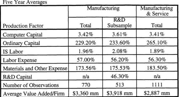
description of the data construction procedure can be found in Appendix A, and summary statistics are shown in Table 1. The basic definitions are given below.
5Specifically, the survey targets Fortune 500 manufacturing and Fortune 500 service firms that are in the top
half of their industry by sales, excluding computer manufacturing firms.
6 Standard & Poor's Compustat data has been widely used to estimate firm-level production functions for capital, labor and other inputs. For instance, the underlying data for "The Manufacturing Sector Master File: 1959-1987" maintained at the National Bureau of Economic Research by Hall (1993) is drawn from Compustat.
IDG reports the "market value of central processors" (supercomputers, mainframes and
minicomputers) but only the total number of "PCs and terminals". We added the "market value of central processors" to an estimate of the value of PCs and terminals, which was computed by
multiplying the weighted average price for PCs and terminals by the "number of PCs and terminals" (see Appendix A for details). This approach implies that PCs and terminals account for about 29% of the aggregate value of COMPUTER CAPITAL in 1988, rising to 72% in 1992, which is broadly
consistent with the values reported by Jorgenson and Stiroh (1993).7 While the year-to-year changes should already account for any depreciation, scrappage, or new investments, they will also account for changes in the market price of computer power, which has been declining steadily because of
technological progress in the computer-producing industries. Because the flow of capital services is presumed to be proportional to the real stock, not the nominal stock, it is important to account for these advances, lest computer-using industries be given credit for the advances in computer-producing industries. We make this adjustment by deflating aggregate computer capital by the hedonic deflator for computers reported in (Gordon, 1993) to get a final value of real computer capital used in the estimation.8 Because computer-power available per dollar has been increasing over time, this means that real computer capital has grown more rapidly than nominal computer capital, in contrast to the trend in other types of capital stock.
IS LABOR was computed by multiplying the IS budget figure from the IDG survey by the "percentage of the IS budget devoted to labor expenses...", and deflating this figure. This will provide an estimate of the "physical" units of IS LABOR used.
The variable for LABOR EXPENSE was constructed from the reported labor expense on Compustat where available, or estimated by multiplying the number of employees by an average labor expense per employee for firms in that particular sector (also computed from Compustat). Approximately 65% of firms had LABOR EXPENSE estimated from average annual expense per employee. The final value for LABOR EXPENSE was then computed by deflating this number by the price index for total
compensation and subtracting IS LABOR. Thus, all the labor expenses of a firm are allocated to either IS LABOR or LABOR EXPENSE. As with IS LABOR, this approach will provide an estimate of the
"physical" units of labor used, including differences in skill levels and hours worked, to the extent that the deflator is accurate. However, as noted in Section IV below, we also examined regressions which used the more conventional measure for labor which is simply the number of employees.
7 Jorgenson and Stiroh (1993) present BEA data that subdivides computer equipment spending into subcategories, and shows that PCs were 27% of total computer equipment in 1988.
8In order to apply Gordon's deflator to this data set, we assumed the trend in prices from 1957-1984 continues through 1992 at the same rate of decline.
Computers and Growth: Firm-level Evidence
Total capital for each firm was computed from book value of capital stock, adjusted for inflation by assuming that all investment was made at a calculated average age (total depreciation/current
depreciation) of the capital stock.9 This approach to constructing total capital is consistent with the
methods used by Hall (1990) and Mairesse and Hall (1994). From this total capital figure, we subtract the deflated value of COMPUTER CAPITAL to get ORDINARY CAPITAL. Thus, all capital of a firm is allocated to either COMPUTER CAPITAL or ORDINARY CAPITAL.
The variable for MATERIALS was computed by deflating total expense (i.e. the difference between Sales and Operating Income Before Depreciation) as reported on Compustat by the producer price index for intermediate materials, supplies and components (PM), and subtracting LABOR EXPENSE and IS LABOR as computed above.
We considered two measures of output: SALES and VALUE-ADDED. SALES was computed by taking total sales from Compustat, and deflating by an industry specific (2-digit SIC) price deflator. VALUE-ADDED was computed by subtracting MATERIALS from SALES.
Finally, R&D CAPITAL was computed by taking R&D expenditures from Compustat, and constructing a capital stock assuming a constant rate of depreciation of 15%, using the method and price deflators described by Hall (1990). Annual R&D expense is included in MATERIALS when R&D CAPITAL is not used as a regressor, and is excluded otherwise.
C. Potential Data Issues
There are a number of potential inaccuracies in the data that could have an impact on the results.
Specifically, COMPUTER CAPITAL and IS LABOR may be measured with error because of the difficulty in valuing computers by survey respondents, the assumptions used to estimate the value of PCs, and potential sample selection bias. We may have also understated total stock of COMPUTER CAPITAL and IS LABOR because we employed a relatively narrow definition of computers that may exclude
important components of spending such as peripherals, telecommunications infrastructure, outsourced services and software. Finally, both inputs and outputs were deflated by imperfect deflators, and the use of firm-level data does not eliminate the effects of mismeasuring output, particularly when quality change or other intangible effects are likely to be important.
D. Estimation Procedure
9An alternative measure of capital stock was computed by converting historical capital investment data into a
capital stock using the Winfrey S-3 table. This approach yielded similar results as shown in column 1 of the table in Appendix C. We chose not to use this method to be more consistent with previous studies that employed the "Manufacturing Sector Master File" at the NBER.
The choice of estimation method was based on several important characteristics of the data set. First, because there are repeated observations on individual firms, the error terms for each firm are likely to be correlated between observations, although it is unlikely that the errors between firms are correlated. Second, the data set is an unbalanced panel in which not all firms are present in all years, and therefore the estimation method must be able to provide consistent and efficient estimates in the presence of missing data. Finally, we prefer a parsimonious specification which involves the minimum number of parameter estimates for the variables of interest.
Given these constraints, we chose to write our estimating equation as a system of five equations, one for each year, and apply the technique of "iterated seemingly unrelated regressions" (ISUR): 10
Vi,92= 8jJj 9 + 2 1 log Ci,92 + 02 log Ki,9 2 + P3 log Si,92 + 4 log Li492 + Ei,92 j-1
Vi,91 = s,- J + 9 + log C,9 1 + 2 log Ki,l + 3 logSi,91+ 4 log Li,91 + i,91 j-1
Vi89 = '
6jJ
+ 890 + p1 log Ci,90 + 02 logKi90 + P3 logSi ,90 + 4 log Li,90 + 8i 90
j-I
Vi,89= 8 5jJj + 89 + 31 log Ci,89 + 2 log Ki,8 9 + 03 logSit89 + 4 log Li,89 + i,89
j-1
Vi,88= E iJj + 88 + 01 log Ci,88 + 2 lo°g Ki,88+ 3 log Si88 + 4 log 4Li88 + -i,88
j-I
The ISUR procedure iteratively computes a feasible generalized least squares estimate for the system with an estimated error term covariance matrix of the form:
Var(e) =
X,
Ildentity(rank =#of firms)where: t is an estimate of the time dimension covariance for a single firm.
In order to minimize the number of parameters to be estimated, we constrain all the elasticity
parameters to be equal across years. This implicitly assumes that the production functions of all the firms are on the same "surface" except for multiplicative shifts associated with the dummy variables. This assumption is more plausible for the manufacturing subsample, which makes up the majority of
our data set, than for the full sample. The separate dummy variable for each year (e.g. 92) picks up the effects of disembodied technological change and other exogenous effects that affect overall productivity, and the dummy variables for each 2-digit industry,l1 the (j) account for systematic
overall productivity differences between industries or sectors. The ISUR procedure allows for any 10This method is a variant of maximum likelihood (ML) and is also known as the Iterated Zellner Efficient
estimator (IZEF). Our software enabled us to use this approach despite some missing data, through the use of "pairwise-present" calculation of covariance matrices. The estimates on a fully-balanced sample of 55 firms are reported in Appendix C and are consistent with our findings for the broader sample.
Computers and Growth: Firm-level Evidence
form of serial correlation between the various years including the structure implied by random firm effects, and also corrects for heteroskedasticity in the time dimension.
IV. RESULTS
In this section, we 1) present estimates of the output elasticity of each of the factors of production, 2) estimate the robustness of the production function estimates to potential simultaneity, 3) extend the analysis to include R&D as a distinct input, and 4) examine an alternative approach based on Solow residuals.
A. Basic Estimates of the Production Function
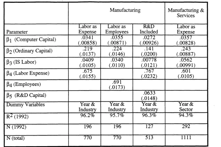
The estimates for the basic value-added equation are given in Table 2, column 1. For manufacturing firms, the elasticity of COMPUTER CAPITAL is .0341, with an asymptotic standard error of .00858. The elasticity of ORDINARY CAPITAL is .219, with a standard error of .0137. To determine whether these estimates imply excess returns to computers, we compare the implied gross marginal products 1
2-with the Jorgensonian cost of capital for computers (Christensen and Jorgenson, 1969). As calculated in Appendix B, the cost of capital is approximately four times higher for computers than for other types of capital, owing mainly to the large price declines in computers and the resulting capital losses from owning COMPUTER CAPITAL. However, the elasticity estimates imply that the gross marginal product for COMPUTER CAPITAL is nearly ten times higher than for ORDINARY CAPITAL, and the data reject the hypothesis that computers are earning the same net rate of return as other capital in favor of the hypothesis that the returns to computers contribute disproportionately to output (p < .02).
The elasticity of IS LABOR, .0409, is over double its factor share. When compared to the elasticity of ordinary LABOR, this suggests that dollar for dollar, IS workers contribute twice as much to value-Added as other types of workers. If computer-intensive firms are disproportionately in industries that use skilled labor, then our use of labor expense, instead of simply number of employees, should help account for this difference. Interestingly, however, as reported in Table 2, column 2, the estimates are qualitatively similar when the number of employees is used directly for ordinary labor input.13
1 2
A estimate of the gross marginal product for a representative firm can be directly calculated from the production function estimates and other sample information:
MQ Q
MPc = Q = 1 Q where Q and C are the mean input and output quantities.
13 Because average labor expense per employee had to be estimated from industry data for many of the firms in our sample, our Labor expense variable will not fully account for differences in labor compensation among firms within the same industry. Such differences may be correlated with the use of computers (Krueger, 1991).
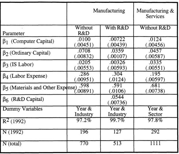
The regression for real SALES reported in Table 3 shows that all of the elasticities are lower when materials are added as an input. Nonetheless, the implied gross marginal products for COMPUTER CAPITAL, ORDINARY CAPITAL and IS LABOR remain fairly similar to those estimated in the value-added specification, since each factor is a proportionately smaller share of SALES than of
VALUE-ADDED.
The right hand sides of Tables 2 and 3 present the results for the full sample, which also includes service firms. The results are similar qualitatively, although the output contributions of computers appear to be even higher and the overall fit is not quite as good. 14 We also compared our ISUR
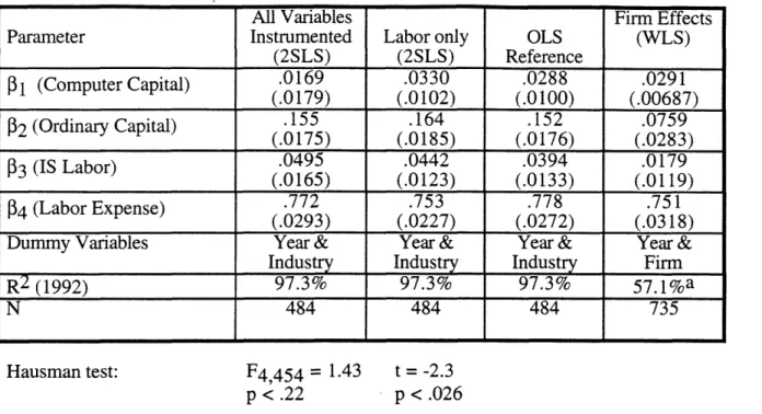
estimates to those of a pooled OLS specification, and found that the elasticity estimates for COMPUTER CAPITAL generated by OLS are comparable or higher than the estimates provided by ISUR (Table 4). For each of the specifications, the elasticities sum to approximately one, implying nearly constant returns to scale.15
The most striking aspect of these results is the high implied marginal product of COMPUTER CAPITAL and the evidence of excess returns. There are at least three explanations which can reconcile this finding with the presumption that profit-maximizing firms should equate the marginal products of all their inputs.
First, our estimates may reflect a simultaneity bias. Investments in COMPUTER CAPITAL, and all other inputs, are in part determined by output, as well as vice versa. Depending on the nature of these relationships, this can bias up or down the estimates of any given input. For instance, if managers of productive firms have a disproportionate "taste" for spending new revenues on high technology, then our production function estimates for computers will be too high. This issue is explored further in the next subsection.
Second, our simple Cobb-Douglas specification ignores many other determinants of output. This will not matter if they are all uncorrelated with the included regressors, however, some may be both correlated with productivity growth and with the use of computers. The most obvious candidate for such a missing variable is R&D, and this possibility is explored in subsection C.16
14 There is insufficient data to estimate consistently a separate production function for service firms only.
15The VALUE -ADDED regressions in manufacturing range between .97 and 1.0 for returns to scale. The SALES
regressions range from .99 to 1.0.
16 A subtler issue is the possibility that our sample is somehow biased to disproportionately include productive users of information technology, in which case our findings could not be extrapolated to the rest of the
Computers and Growth: Firm-level Evidence
Finally, given the rapid changes in computer technology, we think it unlikely that computer capital stock has reached its equilibrium level. On the contrary, the continuing increase in investment and in stock suggests continuing diffusion and adjustment. It has been argued that the excess private returns found for R&D in some studies can be explained by such a diffusion process (Griliches, 1986). This argument seems germane in the present case as well, although it is difficult to test directly.
B. Simultaneity
While the above results indicate a strong correlation between computers and output, they cannot establish causality. Investments in each of the factors of production are affected by past output and profit, as well as expectations about the future, violating the exogeneity assumption of ISUR. Furthermore, if some of the inputs are measured with error, the parameter estimates will be biased. It is possible to examine the characteristics of the potential simultaneity bias by explicitly modeling the relationship between investment and output. There are at least two ways of approaching this problem. Griliches (1979) shows that by adding the assumption of profit maximization, investment becomes a function of current period output, input prices, and other exogenous factors. Alternatively, the investment literature presents several alternative relationships between investment and output, most of which write investment as a function of current and lagged output, in addition to other exogenous variables (Berndt, 1991). Either approach yields the following production-investment system: 17
log
Q
= Po + p log C + P2 log K + /3 log L + eq (production) log C = a, + ac log Q + ac Z, + E, (investment) log K = ak + akq log Q + ckZk + Ek (investment) log L = a, + aq log Q + ca,,Z + e (investment)where: the Zs are matrices of exogenous variables for each equation
In principle, the asymptotic bias in the estimated elasticity of COMPUTER CAPITAL can be determined for this system. However, the actual bias is a function of the as, the Zs and the correlation structure of the error terms in the system, most of which are either unobservable or unknown due to lack of information. In addition, even the sign of the bias is not easily determined. For example, in a very
17
This is a general relationship consistent (at least to a linear approximation) with both the investment literature or profit maximization. For the investment equation, the Z's could include lagged output, cash flow, Tobin's Q or other common measures. For profit maximization, the Z's include prices of output and inputs, the true elasticities and possibly demand characteristics. Note that we have dropped IS labor from the production function to ease exposition.
restricted special case of this system, in which COMPUTER CAPITAL is the only endogenous variable (thus reducing the four equation system to two equations) the sign of the bias is:18
Sign(310oLs -f,) = Sign[cov(e1, c) + acq Var(ec)]
This expression will tend to be positive, since the right hand term is positive. However, if the cross equation correlation is negative and the investment effect of output on computers (xcq) is not too large, the overall bias can also be negative. This could occur if computer investment tends to adjust slowly to random output shocks. For example, if a negative shock to output lowers the required amount of capital, but computer capital persisted, this would result in a positive error in the investment equation correlated with a negative error in the production equation. 19
There are a number of approaches to removing this bias, although none of them is wholly satisfactory. As a result, most of the growth accounting studies using the production function approach have not attempted to address this problem. Nonetheless, we explore possible approaches below: instrumental variables, firm effects, and a combination of the two.
The first, and most common, "solution" to both simultaneity and errors in variables is to identify the exogenous variables (Z) in the investment equations, and use these as instruments to estimate the production equation using an instrumental variables estimator. However, it has proven difficult to identify appropriate variables in the investment equations that are truly exogenous in firm-level data. One possibility is to use lagged values of the endogenous variables as instruments, since by definition, they cannot be correlated with unexpected changes in output in the following year. We are able to apply a two-state least squares2 0 (2SLS) to a pooled data set and compare the results to estimating the system by a single equation using OLS (Table 4). A Hausman test using lagged dependent variables
18This equation is a simplification of Bronfenbrenner's (1953) derivation of bias for two simultaneous
equations. The full equation (restated in our notation) is: (1-fplacq )[cov(EEe)+ acq Var(Ec)]
E(3 -3 1)=
Var(a cq 1+ E) + Var(.)
where the unspecified term in the denominator is a function of the exogenous variables. Thus, the denominator is always positive and the first term in the numerator is also positive yielding the relation shown in the text. A further discussion of this equation is provided by Schmalensee (1972), p. 102.
19 The relative sensitivity of computers to output shocks is unclear. On one hand, because the ratio of
computer investment to computer capital stock is larger than the ratio of ordinary capital investment to ordinary capital stock, computer capital stock may vary more with current output. On the other hand, Fazzari and Petersen (1993) show that fixed investment is considerably smoothed relative to cash flow shocks, with working capital absorbing the difference. Indeed, contemporaneous business analysts argue that computer investment should not be driven by short-term economic considerations, e.g. Mead (1990).
2 0We did not use three-stage least squares (3SLS) to construct parallel estimates to compare to our ISUR results
because the lagged endogenous variables for one year (say 1991) are the actual variables in the previous year (1990). This violates as assumption of 3SLS that instruments are uncorrelated with error in all equations.
Computers and Growth: Firm-level Evidence
as instruments does not reject the hypothesis that all inputs are jointly exogenous. However, the Hausman test cannot reject endogeneity of the LABOR input variable alone. When this variable is instrumented by the other exogenous variables and lagged LABOR, the coefficients on COMPUTER CAPITAL and IS LABOR are little changed -- the elasticity of COMPUTER CAPITAL rises from .0288 (OLS estimate) to .0330 (2SLS estimate). This provides evidence that our results are not driven by the assumption of exogenous inputs. However, a weakness of this approach is that lagged dependent variables are not exogenous if they are serially correlated.
An alternative instrumental variables approach is to use first differences or "long differences" to identify the production equation. Estimation using first differences yields nonsensical parameter estimates, and the data set is too short in the time dimension to use long differences without substantial sample size reduction. Our problems with first differences are not surprising or uncommon since it is known that differencing the data can magnify random measurement error (Griliches and Hausman,
1986; Hall, 1993).
The second possible approach is based on the observation that under certain assumptions, estimates of a firm effects specification can provide consistent estimates in the presence of simultaneity. Following Griliches (1979), suppose that output is influenced by both permanent and transitory shocks. In theory, investment should be affected by the permanent, firm-specific component of output, but not by transitory changes in output resulting from demand variation . As a result, we can rewrite the system of equations:
logQi,, = o + P1 log Cit + 2 log Ki,t + P3 logLit + q,i + q,i,t
log Cit = a + acq log(Qot + qji) + ac*Zc + c,i,t
where £q -q i+ q,i,t
£qi is the permanent component of firm productivity or output shocks,
Cq,i,t is the transitory component,
and, Q?, is the portion of output explained by the inputs.
In our modified investment equation, computer investment is not a function of the individual error component (q i,t) in the production equation. However, because it is a function of the fixed
component of output ( q,i), it will be correlated with the error term in the production equation, and this will introduce bias into the estimate of the elasticities (). To remove this bias, we can estimate the equation including a firm specific intercept which absorbs the fixed component:
log Qi,t= jiIi -E + , log C,, + 2 log Ki, + 3 log Li,, + q,it
where:
pi = Po + q,i', is the firm -specific intercept, and Ii = 1 if observation is firm i, 0 otherwise
This is the traditional fixed effects or within-groups estimator which is unbiased and consistent (although not necessarily efficient) regardless of whether the individual effects are correlated with the other regressors.2 1
An added benefit of the firm effects approach is that it will address the missing variable bias that could result from any other firm differences that are not captured by our production function specification. For instance, if managers of high performing firms also tend to invest heavily in computers, then the basic ISUR estimates of the returns to computers would be biased upward. However, if the
management of firms changes relatively infrequently, then their effect will be subsumed into the firm-specific intercept, so the firm effects estimator will be unbiased.
As shown in the right hand side of Table 4, the estimate for the elasticity of COMPUTER CAPITAL falls somewhat when firm-effects are controlled for (.0291 versus the comparable estimate of .0327 for the same sample (not shown)2 2). The coefficient is still highly significant, both in an OLS regression, and when weighted least squares (WLS) is employed to correct heteroskedasticity in the time
dimension (the WLS results are shown in Table 4). However, the elasticity of IS LABOR is reduced substantially (about 30% of the original). This may suggest that much of the excess return to this factor may be attributable to firm differences, although it may also be due to the fact that within-firm estimates can be biased down by errors in variables (Griliches and Hausman, 1986).
Finally, while the firm effects approach addresses a portion of the simultaneity problem, it is not fully satisfactory if some of the "transient" portion of demand shocks also influences the demand of
computers. In principle, if we apply instrumental variables to the firm effects specification, most of the endogeneity should be eliminated. However, our attempts using lagged endogenous variables proved unsuccessful due to poor fit in the first stage regressions, resulting in meaningless 2SLS
21 Adding an intercept for each of the firms in our sample would involve estimating several hundred additional parameters, which is beyond the capability of our econometric software. Fortunately, there is an alternative approach: the firm effects specification can also be estimated by subtracting a firm-specific mean from each variable. This will remove the firm effect in a similar way to removing the overall regression intercept by taking the mean of all variables. The individual firm effects can be recovered by plugging in the firm specific variable averages into the estimated regression and calculating the residual.
22 The firm effects specification results in some sample size reduction because the analysis was restricted to firms with at least two data points in the sample. This causes the reduction from 770 points to 735 points.
Computers and Growth: Firm-level Evidence
estimates. This problem was foreshadowed by Griliches (1986), who commented that this approach would probably not be successful since growth rates tend to not be correlated over time in firm-level data.
In summary, while the application of both firm effects and instrumental variables simultaneously demands too much of the data and does not yield meaningful results, applying the techniques separately does provide further support for the robustness of our results, particularly the estimate of the elasticity of COMPUTER CAPITAL.
Given the fact that computer systems generally involve numerous complementary components, often including changes in business processes, and lead only indirectly, via better information processing, to increases in output, we think it unlikely that firms rapidly change their computer capital purchases in response to transient changes in demand, and our 2SLS results are consistent with this view.
However, because endogeneity can never be completely ruled out when statistical correlations are found, one interpretation for our results is that we have found a "marker" in the form of computer investment, indicating those firms undergoing significant productivity improvements, but not necessarily causing the improvements. Indeed, Milgrom and Roberts (1990) argue that "modern manufacturing" involves a host of complementary activities, of which advanced technology is only one. It may be that firms which have switched to a new paradigm of production are able to increase their value-added without proportionate increases in inputs. Because numerous complementary changes in organization, capital and labor may be required for such a switch, it could be misleading to attribute all of the gains to only one of those factors, in this case computer capital.23 A more complete
analysis would seek to identify and measure the other posited inputs to "modem manufacturing" or "modem service" and include them in the production function as well. In the meantime, it should be clear that our results should not be interpreted as "proving" that computers contribute
disproportionately to output, but rather as presenting some primafacie evidence in support of such an interpretation.
C. R&D as an Input
Howell & Wolff (1993) have noted that "the production and distribution of information has become the central feature of advanced economies" and argue that this may in part be due to the transition to a "new 'techno-economic paradigm' based on microprocessor driven technology." Therefore, there is a danger that computer use may be correlated with an omitted variable pertaining to the "production of
23 Whether this introduces a "bias" depends, first, on whether computers are necessary for such concomitant changes, and second, on whether one is interested in the partial derivative of output with respect to computers, holding all else constant, or the total derivative, including indirect effects.
information". While it is beyond the scope of this paper to examine the relationship between
computers and all forms of information creation and dissemination, it is certainly true that those firms who are the most aggressive users of technology may also be the most aggressive compilers of R&D capital, and omitting R&D as a distinct regressor could lead to a biased estimate of the returns to COMPUTER CAPITAL and IS LABOR. In fact, Dunne (1993) found that spending on R&D was positively related to the use of computer-based factory automation in a Census Bureau sample of manufacturing firms.
Since R&D spending data is available for many of the publicly-traded firms in our sample, we were able to assess production functions with R&D as a distinct input. In this way, we can also directly compare the results on computers with the larger stream of research on the output contributions of
R&D:2 4
Vi = y(jJ + X6T, + 1llog Cit +]p2 log Kit +P3 log Si, +04 log Li, fl6 logR +-ei
j t-1
where: V, C, K, S, L, T, J are as before R is R& D capital stock
Except that COMPUTER CAPITAL and IS LABOR are distinguished from ORDINARY CAPITAL and LABOR, the above equation is essentially equivalent to the models used in the literature on R&D productivity (see e.g. Hall, 1993) and may contribute to that research tradition. For instance,
Griliches and Berndt, in separate comments on Hall (1993), speculate that the decline in the measured private returns to R&D in the 1980s may be related to the concurrent proliferation of computer
technology.
The results for this equation are reported in Table 2, and the analogous regression on real SALES is reported in Table 3. The elasticity of COMPUTER CAPITAL falls slightly in both specifications when R&D is included, although the difference is less than the standard error of the estimate in either
regression. The elasticity of ORDINARY CAPITAL also falls while the elasticity of LABOR (and material in the sales equation) rises slightly. The coefficients on R&D imply a gross return to R&D of around
15% in the value-added equation and around 30% in the sales equation. Interestingly, the inclusion of R&D CAPITAL dramatically reduces returns to IS LABOR, so that in neither specification can the elasticity of IS LABOR be distinguished from zero. This may be a result of the correlation between IS LABOR and R&D spending, where our high returns to IS LABOR originally picked up some of the effects of R&D CAPITAL stock.
24
We also ran the regression using real SALES and adding MATERIALS as a regressor. In this case, R&D spending was subtracted from MATERIALS to avoid double counting it. Because R&D data were reported by only 6 firms in the service sector, we limited this analysis to manufacturing firms.
Computers and Growth: Firm-level Evidence
For comparison with earlier research on the returns to R&D CAPITAL, such as (Hall, 1993), we also examined a production function which did not distinguish COMPUTER CAPITAL and IS LABOR from ORDINARY CAPITAL and LABOR, respectively. In this specification, the elasticity of R&D CAPITAL was .0774, implying a private rate of return of 16.7%. This is in the low range compared to prior studies which did not explicitly consider COMPUTER CAPITAL and IS LABOR, but not far from the 20.3% rate of return for R&D reported by Hall (1993) for a similar sample of firms over the 1986-1990 time period. Our slightly lower result could show a (further) drop in the rate of return to R&D in the early 1990's, or may just be indicative of sample differences.
While the elasticity of R&D is little affected by whether or not COMPUTER CAPITAL is treated as a separate regressor, this does not directly address the question of whether high IT spending is
associated with lower returns to R&D. A more direct examination of the potential link is provided by comparing the R&D elasticities of firms with high levels of COMPUTER CAPITAL with firms that have less COMPUTER CAPITAL. We divided the firms in our sample into two groups based on the ratio of COMPUTER CAPITAL to LABOR. We found that firms with proportionately more COMPUTER
CAPITAL did not have significantly different R&D elasticities from firms with less COMPUTER
CAPITAL (t = 1.29 for a coefficient difference test). A similar comparison of firms with high and low ratios of COMPUTER CAPITAL to ORDINARY CAPITAL also found no evidence of differences in R&D elasticity (t = 0.83). Of course, Hall's main finding was a decline in R&D returns over time, and our cross-sectional comparison does not really bear on the possibility that computers have facilitated
inter-firm dissemination of R&D knowledge, and thereby lowered private returns to R&D spending. D. The Correlation of Computer Capital with the Solow Residual
As a further robustness check of our results we also compute the contribution of computers through an alternative approach using Solow residuals (Solow, 1957). The residual can be defined as:
Residuali, = log Vit - C V log Ci t - 7cK I log Kit - VtI S Sit -l -og R log R
v,
I
VI
V
IVI,
where: V,C,K,S,L,R, i, and t are as before
IT - factor - specific cost of capital or labor
The residuals for each observation can then be regressed on COMPUTER CAPITAL, and IS LABOR, as well as industry and time dummies:2 5
2 5
This estimating equation is similar to that used by Siegel and Griliches (1991) on industry-level data, except that they report estimates for MFP growth rather than MFP level. Estimating this equation for MFP growth is
Residuali, = y, log C, + y2logSi, + 73 logR, + .gT, + Y.J, + e
t
j-where: Residual, C, and S are as before
Tiand Jj are time and industry dummy variables
If 71, Y2 or y3 are greater than zero, this indicates that the corresponding factor is positively correlated with the Solow residual, or multifactor productivity.
This approach avoids one potential problem of the production function estimates. If for some reason (such as errors in variables), the elasticity of capital or labor were incorrectly estimated, this could lead to a bias in the estimates of the contribution of computers. By explicitly setting these elasticities to their factor shares, as expected in equilibrium, we can evaluate the effects of computers without this bias.
To estimate this equation, we make the usual assumption that the cost of labor, ftL, is 1, thus setting the elasticity to the factor cost share. However, as discussed in Appendix B, the cost of capital is a function of a number of determinants including the real interest rate and depreciation rates, which are not known precisely. Lau and Tokutsu (1992) and Lichtenberg (1993) use estimated values of 7% for the cost of ORDINARY CAPITAL, while our calculations indicate it may be closer to 10% (Appendix B). Likewise, the elasticity estimates presented in Table 2 imply a gross return of approximately 10%. Nonetheless, because the size of the residual will be sensitive to the precise value chosen, we conduct the analysis for several estimates of the cost of capital ranging from 7% to 25%. In addition, the net cost of COMPUTER CAPITAL may also vary over a wide range, so six values are considered (Table 6a). Finally, we repeated the analysis with R&D treated as a distinct factor in both equations (Table 6b).
In this specification, the correlation of the residual with COMPUTER CAPITAL, y1, appears to be relatively insensitive to the assumed cost of COMPUTER CAPITAL, tc, presumably because computers are such a small share of inputs that their costs do not affect the residual much. The size of the
residual, and therefore the estimated excess returns, is more sensitive to the assumed cost of ordinary capital. Nonetheless, there appear to be excess returns to COMPUTER CAPITAL for all but the most extreme values (25% cost of ORDINARY CAPITAL, 50% cost of COMPUTER CAPITAL). For example, if the cost of ORDINARY CAPITAL is assumed to be 20% per year and the cost of COMPUTER CAPITAL is 40% then the coefficient on COMPUTER CAPITAL is .0224. This result implies large, positive excess returns that are comparable to those obtained in the production function estimation. As with the
equivalent to using first differences, which on our data set yields nonsensical estimates, most likely because of our relatively short panel and errors in variables.
Computers and Growth: Firm-level Evidence
production function, these results show that the returns to IS LABOR are attenuated by the presence of R&D CAPITAL as a regressor, with the contribution indistinguishable from zero at a 15% or greater cost of ORDINARY CAPITAL.
V. GROWTH ACCOUNTING
Using estimates from our production function approach, it is possible to determine how much growth in output over the sample time period can be attributed to computers. This can be accomplished in two ways. The first is to examine how the time dummy of the production function changes over time with and without computers as an input. The second approach is to use the elasticity estimates of the various production factors and the growth rates of factor inputs to estimate the growth contribution of each factor, including computers.
A. Effect of Computers on the Trend of Technological Progress
The time dummy on production function regressions is often interpreted as a measure of MFP. This measure of technical change will be affected by any shift in the production function not explicitly accounted for in inputs, including changes in the quality and composition of the capital and labor inputs and especially in the short run, macroeconomic booms and busts. To control for business cycle effects, we include capacity utilization in our regression analysis.26
Vi = E ,jJj + J ST, + 1 logCi,t + P2 logKi., + 3logSi,t + 4logLi,t + vt + i,
i t-l
where v is capacity utilization.
To determine the effect of computers on productivity, we first compute MFP under the assumption that COMPUTER CAPITAL and IS LABOR are no different from ORDINARY CAPITAL and LABOR and can therefore be aggregated. This provides a "base" level of MFP growth over time. We then recompute MFP growth with COMPUTER CAPITAL and IS LABOR as separate inputs. If technological progress, above and beyond the embodied quality-adjustment, is correlated with COMPUTER CAPITAL or IS LABOR, then the change in MFP will be attenuated when these inputs are included explicitly in the production function.
26 This adjustment does not affect the estimates of any of the other coefficients or their preceding interpretations. To the extent, however, that capacity utilization does not account for all the "exogenous factors", error could be introduced in the MFP estimate, but since we only focus on differences between two sets of MFP estimates, the magnitude of this error is likely to be small.
The MFP changes are plotted in Figure 3. When COMPUTER CAPITAL and IS LABOR are included as separate factors, MFP growth drops by either 3% or 5% over the five year period, depending on whether we also include R&D as an input. This suggests that up to 1% per year of growth in VALUE-ADDED can be attributed to advances embodied in computer technology.
B. Growth in Inputs
A second approach is to compute the contribution of each input and technological progress separately, using full production function estimates that include computers as inputs. By taking a first difference between Cobb-Douglas production functions in adjacent years, we can write the following
relationship:
A log V = AMFP + ,A, log C + 2A, log K + f 3A, logS + 4A, log L + A, v
where: V, C, K, S, L are annual firm averages, and v is capacity utilization.
Thus, the contribution of each input to growth in VALUE-ADDED (in percent) is equal to the percentage change of the input multiplied by the elasticity.
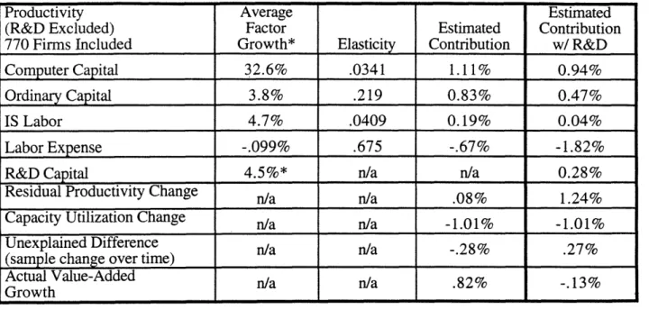
The details of this calculation are shown in Table 7. The analysis is repeated with and without R&D CAPITAL as one of the inputs. Overall, when R&D is not included, COMPUTER CAPITAL adds an additional 1.11% per year and IS LABOR adds an additional .19% per year to growth in value added. This compares with .83% for ORDINARY CAPITAL and -. 67% for LABOR (which was decreasing over the sample period). The MFP residual was .08% per year, after accounting for capacity utilization. This suggests that because of the extraordinary growth in COMPUTER CAPITAL averaging over 30% per year, and the high returns to computer capital investment, computers alone contributed more to output growth than all other capital combined. Interestingly, when R&D is included in the analysis, COMPUTER CAPITAL is estimated to contribute over three times as much to output growth as R&D (.94% per year for COMPUTER CAPITAL vs. .28% for R&D CAPITAL).
Overall, using either method, we find evidence that computer investment has added approximately 1% per year to the growth in gross output over the time period considered. While this is a very large number, it reflects in part the higher cost of capital for computers versus other types of capital
equipment. As capital budgets become increasingly computer-intensive, this necessitates a higher rate of gross capital formation and therefore gross output growth just to maintain the same net growth. Furthermore, as discussed in Section IV, this number will be an overestimate to the extent that
simultaneity and firm effects are important. Finally, these estimates do not take into account spillovers between firms, which may be either positive or negative.
Computers and Growth: Firm-level Evidence
VI. CONCLUSION
We have examined the role of computers in output growth. Our approach was to use recent, firm-level data to estimate the parameters of several production functions. We decomposed capital into three types: ORDINARY CAPITAL, COMPUTER CAPITAL and R&D CAPITAL; and we decomposed labor into two types: ORDINARY LABOR and IS LABOR. In some of the production functions we examined, we also included terms for materials. The models were estimated as a system of five annual equations on individual firm data from a total of 367 firms for the time period 1988-1992.
We found the COMPUTER CAPITAL and IS LABOR made large and statistically significant contributions to the output of the firms in our sample. Considering the relatively small factor shares of COMPUTER
CAPITAL and IS LABOR, their implied gross rates of return are quite high. In fact, these two factors appear to have added 1% to the annual growth in the value-added produced in our sample over the 1988-1992 time period. It appears we are finally beginning to see computers in the productivity statistics, and not just on our desktops.
The high returns implied by our elasticity estimates are not consistent with economic equilibrium. There are a number of possible explanations, with varying implications. First, the costs of computer
capital may be very high, so the net returns could be substantially lower than the gross returns. Second, econometric techniques can generally only determine correlation, not causality. The
association of high returns with computer capital may be due to another unmodeled factor that "causes" both high returns and investment in computer capital. The results from the instrumental variables regressions, the firm-effects regression, and the regression including R&D each address some of the most likely sources of bias, but each of these corrections is imperfect. Third, it is possible that our results are an artifact of the data set that we used. In particular, our sample period was relatively short and involved a period of significant "downsizing" and restructuring.
There are also at least three explanations that leave the door open to the possibility that computers create a disproportionate contribution to output and growth. First, if the benefits and costs of computers are difficult to measure even with hindsight, they must have been even harder to predict. The high ex post marginal product for computers found in our study does not necessarily imply that the expected marginal product, ex ante, was abnormally high. In other words, while the rates of return for all inputs should be equal in long-run equilibrium, the presumption of equilibrium may not be entirely accurate for computer capital. Second, the fact that capital assets cannot be instantaneously scrapped without losing value implies that, even in equilibrium, more productive assets will coexist with older assets until the diffusion is complete. The sharply increasing levels of real investment in