HAL Id: hal-01383970
https://hal.archives-ouvertes.fr/hal-01383970
Submitted on 19 Oct 2016
HAL is a multi-disciplinary open access
archive for the deposit and dissemination of
sci-entific research documents, whether they are
pub-lished or not. The documents may come from
teaching and research institutions in France or
abroad, or from public or private research centers.
L’archive ouverte pluridisciplinaire HAL, est
destinée au dépôt et à la diffusion de documents
scientifiques de niveau recherche, publiés ou non,
émanant des établissements d’enseignement et de
recherche français ou étrangers, des laboratoires
publics ou privés.
A soft route toward 4D tomography
Thibault Taillandier-Thomas, Stéphane Roux, François Hild
To cite this version:
Thibault Taillandier-Thomas, Stéphane Roux, François Hild.
A soft route toward 4D
tomogra-phy. Physical Review Letters, American Physical Society, 2016, 117, pp.025501.
�10.1103/Phys-RevLett.117.025501�. �hal-01383970�
Thibault Taillandier-Thomas,∗ St´ephane Roux,† and Fran¸cois Hild‡
Laboratoire de M´ecanique et Technologie, ENS Cachan/CNRS-UMR 8535/Univ. Paris-Saclay, 61 Avenue du Pr´esident Wilson, 94235 Cachan cedex, France
(Dated: June 15, 2016)
Based on the assumption that the time evolution of a sample observed by computed tomography requires much less parameters than the definition of the microstructure itself, it is proposed to reconstruct these changes based on the initial state (using computed tomography) and very few radiographs acquired at fixed intervals of time. This paper presents a proof of concept that for a fatigue cracked sample, its kinematics can be tracked from no more than two radiographs in situations where a complete 3D view would require several hundreds of radiographs. This two order of magnitude gain opens the way to a “computed” 4D tomography, which complements the recent progress achieved in fast or ultra-fast computed tomography, which is based on beam brightness, detector sensitivity, and signal acquisition technologies.
PACS numbers: 81.70.Tx; 87.57.Q-; 06.30.Bp
Away from medical and biological applications [1], 3D imaging has revolutionized materials science [2–4]. From imaging aiming at visualization to a more quantitative assessment of material morphology, from synchrotron fa-cilities to lab scale equipments, from several hour scans to ultra-fast acquisitions lasting no more than a frac-tion of a second, X-ray Computed Tomography (XCT) is becoming an easily accessible, friendly and perform-ing technique. For applications such as metrology and nondestructive testing, it is also becoming much more common in industry.
In the recent years, one striking trend is the recourse to 4D imaging to track in time the microstructure of a sam-ple [4–6]. The fantastic achievements (e.g., tomography of metal solidification [5] or even of live flying insects [7]) have been made possible only through the development of fast data acquisition techniques.
It is natural to draw a parallel with the large data flow to be handled in movies. Storing every single time frame on its own is highly redundant. The (t + 1)-frame is usually very close to the (t)-frame and hence storing the complete (t)-frame and the “sparse” difference between times (t + 1) and (t) requires much less data than both images independently as evidenced in movie compression standards [8]. Based on a similar observation, Ref. [9] recently proposed denoising strategies with subset-based restoration techniques in 3D plus time in order to com-pensate for the missing information due to fewer projec-tions. The efficiency of movie compression lies in the “sparsity” of the difference (especially when motion is accounted for) that has to be described in a suited lan-guage. Pushing the analogy into the field of tomography suggests that after the full 3D state of a sample in its ini-tial state has been acquired, it is possible to reconstruct
∗[email protected] †[email protected]
only the differences between two consecutive 3D images from much fewer projections. The present study aims at exploring this route, whereby an enhanced 4D rate would be obtained algorithmically through a specific reconstruc-tion rather than from the acquisireconstruc-tion equipment. Only a single time step is considered in the present paper while further indications for 4D are given in the Supplemental Material [27]. In practice, both software and hardware strategies should be combined rather than opposed to reach extreme time resolutions.
Tomography consists of computing the 3D image f (x), such that for a large set of directions θ, the projec-tion (i.e., integral of the X-ray absorption coefficient) matches the acquired projection p(r, θ) (i.e., cologa-rithm of the beam intensity received at pixel r on the detector, normalized by the beam intensity at the same detector position without sample)
Πθf (x) = p(r, θ) (1) where Πθ is the projection operator.
Mathematically, the reconstruction problem corre-sponds to a Radon transform relating the 3D image f (x) to p(r, θ) that is to be inverted. Solving for f (x) from
p(r, θ) is a well-mastered problem for which different
al-gorithms are known with their respective merits [10]. In discrete form, the sampling in angle θ should be cho-sen such that the maximum displacement of a voxel in
f (x) between two consecutive angular positions should
be smaller than a detector pixel size, thus leading to a number of angles proportional to the diameter of the sam-ple (measured in detector pixels). Hence, a tomographic image whose cross-section is Nx× Nx pixels with e.g.,
Nx = 1, 000 requires usually about Nθ ≈ 1, 600 projec-tions. Algebraic reconstruction techniques can help re-ducing Nθ although it cannot be less than Nx without further assumptions on the image texture.
As a side remark, let us note that prescribing fur-ther constraints on the to-be-reconstructed image such
2 as discreteness of gray levels [11] down to binary
im-ages [12, 13], sparse non-zero pixels [14] or sparse bound-ary between constant value domains [15] may constitute a very efficient way of reducing the number of needed pro-jections, compensating for a lack of projection data with specific a priori assumptions. In contrast, the present study aims to address arbitrary images.
Many different scenarios may be considered for describ-ing the time evolution of a studied sample, a generic cat-egory of which is motion, including deformation. One classical tool used to quantitatively study such an evolu-tion is Digital Volume Correlaevolu-tion (or DVC [17, 18]), an extension to 3D images of Digital Image Correlation [16]. This technique consists of registering two 3D images ac-quired (or reconstructed) at different times, t0 and t1,
by accounting for a displacement field u(x; t1, t0).
As-suming the image texture has only been subjected to a geometrical transformation, the following DVC func-tional operating on an arbitrary displacement field v(x) is introduced TDV C[v] = ∫ (f (x, t0)− f(x + v(x), t1)) 2 dx (2)
Global DVC [19] further constrains the displacement field to be a linear combination of a chosen set of fields φi(x) for i = 1, ..., Nv
v(x) =∑
i
viφi(x) (3)
A general example of kinematic bases well suited to me-chanical modeling is those used in the framework of the finite element method. A mesh supporting finite element shape functions can be used, thereby ensuring displace-ment continuity (higher regularity can be chosen accord-ing to the shape function order). Finally, the displace-ment field is obtained from the minimization of the above functional [16]
uDV C(x; t1, t0) = Argminv(TDV C[v]) (4)
with respect to vector v gathering all unknown ampli-tudes vi. Let us stress that the number of parameters Nv needed to describe the kinematics is always much lower than the number of voxels in the 3D images, opening the way to reducing the number of projections.
Because the reference state is typically the rest state, time is available for carrying out a complete 3D image at time t0 using as many projections as needed to
ob-tain f (x, t0). For later times, only a few projections are
assumed to be available, which would not be sufficient to reconstruct the corresponding 3D volume. For any displacement field v(x), the full 3D image f (x, t0) is
ad-vected to a deformed state that should be compared with known projections. Registration is now evaluated from
the projection based residuals only
TP−DV C[v] = ∫ (Πθf (x− v(x), t0)− p(r, θ, t1)) 2 dx (5) and the Eulerian displacement field is the minimizer of this functional
uP−DV C= Argminv(TP−DV C[v]) (6) Because an accurate computation of the projected de-formed volume is needed, this approach is not easily ex-tendable to “local tomography”.
Such an approach (referred to as P-DVC in the fol-lowing) was originally proposed in Ref. [21] and tested on a simple geometry where the strain magnitude was very small, so that a rigid body motion revealed to be a fair approximation. It was observed that although the basic principles of the methodology were sound, the un-certainty of the measured displacement field was larger along the boundaries of the solid because the mesh had to strictly enclose the actual sample, and because, at the boundaries, phase contrast effects are present although neglected in the reconstruction. Moreover, it was also noticed that fine meshes led to numerical instabilities due to ill-conditioning. Thus, it is legitimate to ask whether the method would resist to a much more difficult test in-volving a complex kinematics and requiring a fine mesh. To make the problem well-posed, the effective number of degrees of freedom has to be reduced, yet it is im-portant to be able to deal with a fine mesh to precisely account for the sample geometry and kinematics. One way to satisfy these two opposite requirements is to con-sider soft Tikhonov regularization [20]. This implies a penalty to be added to the functionalTDV C as the dis-placement field departs from an expected property. Clas-sically, terms like the amplitude of the displacement∥u∥ or of the norm of its gradient are used, although they introduce unphysical bias. It is preferred to introduce a penalty to deviations from the solution to a homogeneous elastic problem [22–24]. Introducing the (infinitesimal) strain tensor ε = (1/2)(∇u + (∇u)t), Hooke’s tensor C that relates stress σ and strain, σ = C : ε, the balance equation in the absence of body forces,∇ · σ = 0, shows that the elastic displacement field obeys the second order homogeneous differential equation∇ · C : ∇v = 0. The choice is made to introduce a penalty on the quadratic norm of the left member of this equation, referred to as the equilibrium gap, which reads
TReg[v] = ∫
∥∇ · C : ∇v∥2
dx (7)
Adding the two contributions TP−DV C andTReg nat-urally selects a length scale. To make it more explicit, and hence easy to tune, a specific displacement orien-tation w0 and wavevector k0 are chosen. Based on the
trial displacement field v0(x) = w0exp(ik0· x) the total functional is written as TT ot[v] = TP−DV C[v] TP−DV C[v0] + (|k0|ξ) 4 TReg[v] TReg[v0] (8) The meaning of regularization length ξ stems from the above expression, namely, at long wavelengths,TP−DV C is dominant and hence image registration determines the displacement, whereas at short wavelengths, the regu-larization length produces a smooth and differentiable displacement field. If a large ξ is not faithful to reality then the residuals will display a large value, motivating for lowering ξ down to values such that the residuals are comparable with the residual level observed for the refer-ence image where the displacement is null. A much more extensive discussion on regularization is provided in the Supplemental Material [27].
Let us stress that the above regularization does not require the specimen to strictly obey linear elasticity. Rather, it may be seen as a filter that dampens abrupt displacement gradients with reference locally to the so-lution to an elastic problem. Let us note that a viscous fluid, a visco-elastic solid, or a material exhibiting plastic-ity, viscoplasticity or a damage behavior would all locally display an incremental relationship between strain and stress rates that has the same algebraic form as that of an elastic problem, with the difference of being spatially heterogeneous. Therefore at the expense of being locally less precise than using a complete mechanical modeling, the above filter appears to be very generic. It is to be noted that the limit of an infinite regularization length
ξ is well-defined, namely, the problem consists of
solv-ing for the minimization of TP−DV C[v], Equation (5), for v in the regularization kernel,TReg[v] = 0. The elas-tic problem itself is well-posed once boundary conditions are set, and hence the problem reduces precisely to the determination of the boundary conditions. The regular-ization length ξ can also be tuned down to small values, comparable to the element size, so that regularization is essentially deactivated. In the first limit, the number of effective degrees of freedom are those accounting for the boundary conditions (i.e., nodes on the surfaces where displacement is to be set), whereas in the second one, all nodes of the mesh have an unknown displacement vector. The limitation of the latter case is that the conditioning of the problem will get poorer as ξ decreases, and a pos-sible remedy would imply an increase of the number of needed projections. Yet, for a very small size such as
ξ = 10 voxels, the number of effective independent
de-grees of freedom is of the order of 300 times less than the number of voxels, thus potentially leading to more than two orders of magnitude gain in the number of projec-tions. The effect of tuning the regularization length is illustrated in the Supplemental Material [27].
The following example describes the application of the proposed strategy to a real test case in order to
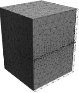
demon-FIG. 1. Nodular graphite cast iron sample and superimposed fine mesh. The sample is in its reference state for a 12 N tensile load
strate that the above strategy works with no more than two projections, and this for a specimen containing a crack where a very fine mesh is to be utilized.
A cast iron sample, containing well dispersed 50-µm nodular graphite particles, was subjected to a cyclic load-ing so that a fatigue crack propagates throughout a large portion of the cross-section. The test was performed
in-situ at the European Synchrotron Radiation Facility
(ID19 beamline, 60 keV energy) so that a series of tomo-graphic images could be acquired at different stages of loading and/or crack growth.
The region of interest size is 1.67× 1.72 × 2.59 mm3 or 330× 340 × 512 voxels, with a voxel size chosen to be 5.06 µm. A full reconstruction requires Nθ = 600 pro-jections. Several volumes were imaged at different load levels (50, 100 and 140 N). In the following the selected pair of states is chosen after 30,000 cycles (close to failure that occurred after 50,000 cycles). The reference state is chosen at a small but non-zero tensile load of 12 N to cancel out possible plays of the tensile stage. The de-formed state was that obtained for the highest load level (i.e., 140 N) for the test to be discriminating.
The trace of the crack was visible on the reference state of the sample and hence it was possible to segment the crack and produce a fine mesh where the two crack faces have been separated. Figure 1 shows the mesh super-imposed onto the microstructure. It consists of 4-noded tetrahedron (i.e., T4) elements with about 2,100 nodes and 8,500 T4 elements. At the crack tip the mesh was re-fined with element sizes down to 15 voxels. Alternatively an X-FEM [25] strategy could have been used.
The minimization of the total functional based on pro-jections is considered. The limit of the regularization length ξ tending to infinity is selected so that the only unknowns are the boundary conditions along the top and bottom faces. The latter sections are moreover consid-ered as rigid so that only 12 unknowns remain to be determined. The number of projection directions (cho-sen to be perpendicular) that are considered is Nθ = 2. Let us stress that imaging the entire volume required
4
FIG. 2. Difference between actual projections of the deformed state and projections of the corrected reference volume. The left and right views are the two projections that are used for P-DVC
more than two orders of magnitude more numerous ra-diographs, Nθ= 600.
The determination of the displacement field was ob-tained from the minimization of the functional Ttot us-ing a Newton-Raphson procedure. Convergence was ob-served to be reached within about 5 iterations only.
One way to evaluate the quality of the procedure is to consider the difference between the two projection im-ages whose quadratric norm is the integrand of Equa-tion (5). These differences, called “projecEqua-tion residuals”, are shown in Figure 2. Qualitatively, it is observed that most features of the projections have disappeared in the residuals, but the projection of the crack whose morphol-ogy is only approximately captured by the mesh, and where phase contrast effects — not modeled in the pro-cedure — are expected. Quantitatively, the gauge to in-terpret faithfully the level of residuals is provided by ap-plying the P-DVC procedure to a deformed state that is chosen as the reference. The displacement is identically null, yet the projection of the reconstruction in the two chosen directions is never exactly equal to the recorded projections because of acquisition imperfections, as well as reconstruction or projection biases. These baseline residual levels amount to a Signal to Noise Ratio, SNR, of about 31.5 dB for the projections. The same estimate for the actually deformed sample leads to a SNR≈ 30 dB which is only about 1.5 dB lower. Hence reconstruction, projection, and interpolation are responsible for most of the remaining residuals, thereby validating the registra-tion process.
The initial claim was that the proposed technique would allow to track the entire 3D volume although only two projections were used. In the discussed example, the entire set of 600 projections had been acquired, so that one may directly compare the reference volume ad-vected by the estimated P-DVC displacement field and the direct reconstruction of the deformed volume. These two volumes and their difference are shown in Figure 3. The difference between the volumes reveals mostly recon-struction artifacts that impact differently the two proce-dures, and slight inaccuracies in the description of the
FIG. 3. (left) Advected reference volume using the P-DVC estimated displacement field; (right) Reconstructed deformed volume; (center) Absolute difference between the two preced-ing volumes
crack geometry from segmentation and meshing. The SNR estimated on the reconstructed volume amounts to 24 dB, to be compared to 25 dB when the displacement field issued from standard DVC (based on volumes), and 30 dB when the proposed P-DVC is applied to the ref-erence volume itself, and the displacement field (that should ideally be 0) is used to “correct” the volume. Sim-ilarly, the RMS difference between displacement fields obtained from P-DVC and standard DVC amounts to 0.18 voxel. The Supplemental Material [27] presents ad-ditional details on the influence of the chosen reconstruc-tion procedure, mesh fineness, or regularizareconstruc-tion length for this experimental example.
It has been shown that considering (even complex) kinematics regularized through an equilibrium-gap elas-tic penalization as a regularization allowed for tracking the time evolution of a loaded cracked sample. In this experimental test case, the number of projections was reduced from 600 down to 2. The low level of residuals and the very good agreement with standard DVC consti-tute a validation of the proposed principle.
The presented analysis is based on the assumption that the temporal evolution of the specimen is due to motion and that this motion can be (at least at small scales) approached by an elastic problem. Cases where the mi-crostructure topology changes — as when a new phase appears (e.g., void nucleation), when two features merge into one (coalescence) or when an unexpected crack ini-tiates — fall out of the scope of the proposed formal-ism. However, it is believed that the general philoso-phy remains valid, namely, provided the evolution can be modeled faithfully, with a number parameters that is much smaller than the voxel number, then matching virtual (computed) projections with a set of few actual projection allows to track the time evolution with few ra-diographs, and hence at a high rate. This methodology opens the way to an enhanced temporal resolution, i.e., 4D tomography, based on a data processing approach and
no change in required equipment.
The support of ANR (“ANR-11-BS09-027 EDDAM” project and “Investissements d’Avenir” program under the reference “ANR-10-EQPX-37 MATMECA”) is grate-fully acknowledged. The tomographic data used in this letter have been obtained at ESRF (European Syn-chrotron Radiation Facility), on beamline ID19, during experiment MA-501, and benefitted from the framework of the Long Term Project HD501. The authors acknowl-edge the precious help of C. Jailin for significantly im-proving the quality of reconstruction thanks to a specific flat-field correction procedure. Reconstruction benefitted from the reconstruction software ASTRA, [26].
[1] Doi, K., (2005). British Journal of Radiol. 78(1), S3–S19. [2] Maire, E., Buffi`ere, J.-Y., Salvo, L., Blandin, J.-J., Lud-wig, W., Letang, J. M., (2001). Advanced Engineering Materials, 3(8), 539–546.
[3] Baruchel, J., et al. (2006). Scripta Materialia, 55(1), 41– 46.
[4] Maire, E., Withers, P. J., (2014). International Materials Reviews, 59(1), 1–43.
[5] Salvo, L., Di Michiel, M., Scheel, M., Lhuissier, P., Mireux, B., Su´ery, M., (2012). Materials Science Forum,
706, 1713–1718.
[6] Ulvestad, A., Tripathi, A., Hruszkewycz, S. O., Cha, W., Wild, S. M., Stephenson, G. B., Fuoss, P. H., (2016) Phys. Rev. B 93, 184105.
[7] Walker, S.M., Schwyn, D.A., Mokso, R., Wicklein, M., M¨uller, T., Doube, M., Stampanoni, M., Krapp, H.G., Taylor, G.K., (2014). PLoS Biol. 12(3), e1001823. [8] Richardson, E.G., (2003) H.264 and MPEG-4 Video
Compression: Video Coding for Next-generation Multi-media, Chichester, John Wiley & Sons Ltd.
[9] Jia, X., Lou, Y., Dong, B., Tian, Z., Jiang, S., (2010). Med Image Comput Comput Assist Interv., 13(1), 143– 50.
[10] Kak, A. C., Slaney, M., (2001). Principles of comput-erized tomographic imaging. Society for Industrial and Applied Mathematics.
[11] Herman, G.T., Kuba, A., (eds.), Advances in discrete to-mography and its applications, Bikh¨auser, Basel (2007). [12] Batenburg, K.J., (2007). J. Math. Imaging Vis. 27, 175–
191; ibid., (2008). J. Math. Imaging Vis. 30, 231–248. [13] Gouillart, E. , Krzakala, F., Mezard, M., Zdeborov´a, L.,
(2013). Inverse Problems, 29, 035003.
[14] Donoho, D.L., Tanner, J., (2010). Proceedings of the IEEE, 98, 913–924.
[15] Cand`es, E.J., Romberg, J., Tao, T., (2006). IEEE Trans. Inform. Theory, 52, 489–509.
[16] Sutton, M. A., Orteu, J. J., Schreier, H., (2009). Springer Science & Business Media.
[17] Bay, B. K., Smith, T. S., Fyhrie, D. P., Saad, M., (1999). Experimental Mechanics, 39(3), 217–226.
[18] Bornert, M., Chaix, J. M., et al., (2004). Instrumenta-tion, Mesure, M´etrologie, 4(3-4), 43–88.
[19] Roux, S., Hild, F., Viot, P., Bernard, D., (2008). Composites Part A: Applied science and manufacturing, 39(8), 1253–1265.
[20] Tikhonov, A. N., Arsenin, V. Y., (1977). Solutions of Ill-Posed Problems. Washington, DC: Winston.
[21] Leclerc, H., Roux, S., Hild, F., (2015). Experimental Me-chanics 55, (1), 275–287.
[22] R´ethor´e, J., Roux, S., Hild, F., (2009). European Journal of Computational Mechanics 18, 285–306.
[23] Leclerc, H., P´eri´e, J.N., Hild, F., Roux, S., (2012). Me-chanics & Industry 13, 361–371.
[24] Taillandier-Thomas, T., Roux, S., Morgeneyer, T., Hild, F., (2014).
[25] Sukumar, N., Mo¨es, N., Moran, B., and Belytschko, T., (2000). International Journal for Numerical Methods in Engineering 48(11), 1549–1570.
[26] van Aarle, W., Palenstijn, W. J., De Beenhouwer, J., Altantzis, T., Bals, S., Batenburg, K. J., and Sijbers, J., (2015). Ultramicroscopy 157, 35–47.
[27] See Supplemental Material [url], which includes Refs. [24–26]
Supplemental Material to ms. LJ14513
Thibault Taillandier-Thomas,∗ St´ephane Roux,† and Fran¸cois Hild‡
Laboratoire de M´ecanique et Technologie, ENS Cachan/CNRS-UMR 8535/Univ. Paris-Saclay, 61 Avenue du Pr´esident Wilson, 94235 Cachan cedex, France
(Dated: May 20, 2016)
I. ELASTIC REGULARIZATION
I.1. A simple 1D analogy
Let us propose a simple analogy in 1D rather than 3D, where the motion is described with a displacement field being a 1D function v(x). Let us assume that the true displacement, u(x), is given, and no specific properties are assumed. The effect of image registration can be mimicked by an “attachment to data” term such as
T1(v) =
Z
(u(x) − v(x))2dx (1)
to be minimized. The elastic regularization in 1D re-duces to a penalty proportional to the norm of the second derivative
T2(v) =
Z
v00(x)2dx (2)
with a weight ω. Then the problem consists of minimiz-ing
Ttot(v) = T1(v) + ωT2(v) (3)
Dimensionally, ω is the fourth power of a length scale. In order to normalize it properly, a gauge function is selected as a pure Fourier mode, v0= e2iπx/λ, so that
Ttot(v) = T1(v) T1(u + v0) +ξ 4 λ4 T2(v) T2(v0) (4) where ξ is by definition the regularization length (this equation can be compared to Equation (8) of the main text).
I.2. Regularization length
An infinite weight ω given to this penalty would enforce u to be an affine function, or in other words, the kernel of T2is not empty. Its dimension is 2, and any boundary
conditions u(x0) and u(x1) for the interval (x0, x1) can
be accommodated to select a unique element from the
∗
kernel. The minimization of Ttotnaturally results in u(x)
being a linear regression through the data v(x).
Similarly, if ω is finite, u(x) can be shown to be math-ematically a low-pass filter applied to v(x), namely pre-serving the long wavelength modulations of v, while high frequencies are dampened to produce smooth variations. Crudely, one may say that at small scales, λ ξ the smooth variation is a way to get closer to an affine vari-ation of u(x) (the kernel of T2), hence displaying a
con-stant strain, although u(x) is not affine over large dis-tances.
The regularized displacement field requires only a coarse sampling (at the scale of the regularization length, ξ) to be accurately described. Thus, for a sample of size L, the number of unknowns scales as L/ξ when ξ L, whereas for a large weight being given to the regulariza-tion, ξ L, the number of unknowns is equal to the dimension of the T2 kernel, 2. It is clear that the
regu-larization can be made arbitrarily flexible at the expense of a larger number of unknowns.
The analogy with the proposed strategy is direct, and only dimensionality matters. An infinite regularization length ξ corresponds to strictly obeying homogeneous linear elasticity. The “equilibrium gap” TRegused in the
paper has a kernel that consists of all displacement fields with arbitrary Dirichlet boundary conditions. A reduced regularization length (i.e., smaller than the sample size L) gives more and more flexibility (as would do a finer mesh). The effective number of degrees of freedom scales as (L/ξ)3 where the third power comes from the space dimensionality.
In the case study that is presented in the manuscript, the choice of an infinite ξ has been made. The Dirich-let boundary conditions are the prescribed displacements on the top and bottom face of the sample. As a further simplification, it is assumed that these faces are simply subjected to rigid body motions, and thus 12 degrees of freedom are to be determined. The displacement along those faces may be more complex, and may involve addi-tional strains. However, the latter are expected to decay as one moves away from the boundary where they are prescribed. The level of residuals shows that it is a good enough approximation for the considered example, allow-ing for the determination of the displacement field with no more than two projections.
II. RELEVANCE OF THE REGULARIZATION
The foundation of the present approach is that changes with time, specialized to the sample motion, requires much less data than the image itself. The higher the displacement complexity, the more numerous projections to be used. For instance, rigid body motion is the most simple set of displacements, but it lacks the versatil-ity needed to encompass a broad class of applications. What is proposed is to refer to the most generic kine-matic model, i.e., an elastic model.
Otherwise, if it is known beforehand that the sample consists of different parts, each of which having different elastic properties, then such a description can be used as a regularization scheme right away. In the same spirit, a more sophisticated constitutive law could also be used instead of linear elasticity, if such an information is avail-able. This emphasizes the fact that modeling is the key to access a reduction in the number of unknowns more than elasticity. The latter is used herein as a decent guess, easy to continuously relax by decreasing ξ, in case of absence of information on the mechanical behavior.
II.1. Applicability to non-elastic deformation
How restrictive is the reference to elasticity for regu-larization? As above discussed, the motion of the sample is sought. This motion is usually produced by forces or torques (generically called loads) being applied to the specimen. Hence the motion is a manifestation of its mechanical constitutive behavior. For a homogeneous medium, the specimen motion will reflect its constitutive law, e.g., elasticity (linear or nonlinear), visco-elasticity, plasticity, elasto-plasticity, visco-plasticity. Similarly, damage coupled to plasticity or visco-plasticity, all give rise to a tangent operator relating stress and strain in-crements that is identical to that of an elastic problem, but with heterogeneous (tangent) elastic properties. This point will be discussed in the next subsection.
Our present experience in the field of Digital Volume Correlation (DVC) is that even if wrong or inaccurate, the elastic regularization turns out to be very useful even for describing plastic strain, up to localized regimes where shear is concentrated into bands and not evenly distributed (see e.g., Ref. [1]).
II.2. Applicability to homogeneous elasticity
Therefore nonlinear constitutive laws can also be cast in the very same category as spatially inhomogeneous elasticity. Limitations will not result from elasticity by itself, but rather from its assumed homogeneity. This is the very reason a scheme is introduced where an internal length scale, ξ, can be used. Its meaning is such that
over such a length scale the tangent constitutive law of the sample is considered as homogeneous, while above it, different behaviors may be at play varying from region to region.
Let us also stress that, for an elastic medium, using a wrong value of the Young’s modulus can be compensated by having rescaled forces applied on the boundaries, with no further consequence in terms of displacement field.
II.3. Consequence of having a small regularization length
By tuning the regularization length, the “complexity” of the displacement field can be adjusted. As ξ is reduced, the number of effective unknowns increases, and when the regularization length becomes too small, more than two projections may be needed to be able to solve the prob-lem. Yet, in all cases, the number of parameters needed to describe the motion will always be much smaller than those needed to reconstruct the full microstructure. For instance, a finite element description of an arbitrary dis-placement field over a regular cubic mesh, with a mesh size of 10 voxels between nodes, produces one thousand times less nodes than voxels. Even considering that the unknown is a vector at nodes, rather than a scalar at vox-els, the ratio is still above 300. Thus, without regular-ization, a small mesh discretization of the displacement field requires 300 times less unknowns to be determined. Elastic regularization is only a ‘smarter’ way to produce a coarse mesh, and because it is often much more realistic, the number of required unknowns for a similar quality is lower. Building on the previously used 1D analogy, the recourse to a coarse mesh would simply consist of constructing u(x) as a piecewise linear and continuous function as an approximation of the displacement v(x), whereas regularization aims at minimizing the norm of the second derivative, thereby producing a more regular approximation for a length ξ comparable to the previous linear element size.
II.4. How should the regularization length be determined?
A general approach is proposed, which is actually fol-lowed in the context of DVC. The first stage consists of measuring the minimum value of residuals that can be expected, and this is achieved as described in the pa-per, by computing the projection residual from the refer-ence volume. This sets the level of residuals that can be reached at best. Then, a first computation is performed with a large value of the parameter ξ, so that very few degrees of freedom are needed, at the potential expense of being inaccurate (because of the heterogeneity or the constitutive law being different from elasticity). Yet the
3 mean displacement is generally well captured and only
medium to high frequency details are missing at places that can be guessed from the projection residuals. These residuals (if higher than those to be attributed to noise or artifacts) may motivate for leaving more freedom to the displacement field and hence reduce ξ down to either convergence to a low enough value of the residuals, or poor conditioning of the inverse problem and thus where the only parry is to add another projection. Experience from DVC is that large regularization lengths can be used for a fairly large class of displacement fields.
III. CASE STUDY
The companion Letter discusses an example, under conditions that lead to a good registration of the two projections used, based upon an “infinite” regularization length, so that the displacement field lies in the kernel of the elastic model. On the two sides where a displace-ment field is prescribed, these fields are further simplified to rigid body motions, so that only 12 degrees of freedom are left.
Many variants can be considered in order to check the robustness of the method.
• Reconstruction: First, the quality of the reconstructed volume is of great importance. Different flat-field nor-malizations and reconstruction algorithms have been tried. An original flat-field normalization based on a principal component analysis of control regions that are never masked in the radiographs was designed (un-published) and proved useful. Algebraic reconstruc-tion (SIRT) from the ASTRA software [2] was used in the companion Letter. When using a Filtered Back-Projection (FBP) reconstruction — a standard refer-ence algorithm — the projection residual for the ref-erence image (prior to any motion) lead to SNR of 22 dB, whereas the algebraic reconstruction provides a much higher value of 41 dB. Those values are esti-mated without any motion correction. If the proposed algorithm is used in order to compute a displacement field (although it should be equal to 0), the RMS norm of the displacement field gives an estimate of the uncer-tainty. In this case, using the same mesh, the displace-ment uncertainty increases from 0.32 vx. to 0.96 vx. respectively for SIRT and FBP.
• Projection angles: The sample cross-section being rect-angular, one choice (termed (0, π/2)) was to choose angles aligned with the principal axes of the sample. A second choice (−π/4, π/4) is to select intermediate values to limit possible phase contrast artifacts. Sur-prisingly, the (0, π/2) choice led to 31 dB as compared to the 27 dB of (−π/4, π/4).
• Number of projections: The latter, np, can easily be
tuned in the test case as the quality of the determined displacement field is anticipated to increase more and more with their number. In the present case, the num-ber of used projections was pushed to the extreme limit of np = 600. There, the quantity of information was
the same as for traditional DVC. However, it was no-ticed that in the reference case, the SNR remains of the same order of magnitude (28 dB) as for two pro-jections only. Thus it is deduced that the quality of the determination is not limited by the amount of available information in the projections, but rather by extrane-ous factors (acquisition artifacts, noise).
• Masks: Because of the expected phase contrast in the vicinity of the crack, a mask procedure is used so that the immediate vicinity of the crack projection is not considered in the residuals. Different masking variants can be considered, either on the reconstructed volume, or fixed on the projections. When initialized by a close enough result, then no significant differences in the SNR at convergence were observed. However, when initialization is far from the actual solution, the mask-ing variants display different performances.
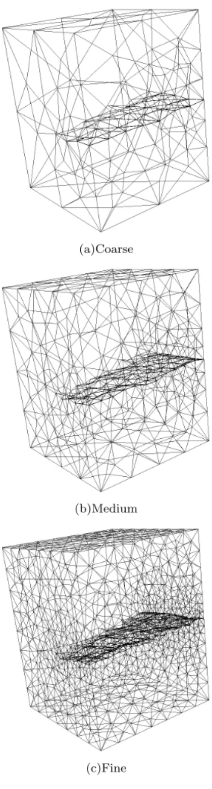
• Mesh size: Three different mesh sizes have been con-sidered, from coarse to fine as shown in Figure 1 (the fine mesh was used in the main body of the Letter). The observed SNR was quite close for the three meshes. Figure 2 shows that very faint differences appear in the displacement fields as the mesh is refined. Whenever the displacement field is not penalized by too coarse a mesh, then regularization makes the mesh size insensi-tive. (The ill-posed character of the problem is cured by the regularization.)
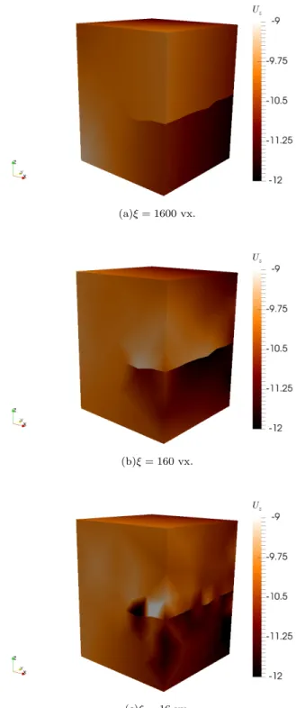
• Regularization: It has been checked on a coarse mesh that relaxing the regularization length to ξ = 1600 vox-els, has no visible consequence. When reducing this length scale further, noise sensitivity becomes clearly visible, especially close to free boundaries, and crack faces, as shown in Figure 3b where ξ = 160 voxels has been reduced by a factor of 10. A further 10-fold re-duction to ξ = 16 voxels (Figure 3c) leads to manifestly unphysical displacements especially close to the crack faces.
This procedure is more costly, as the number of de-grees of freedom increases but it clearly demonstrates the benefit of regularization. Not only does the dis-placement look more regular (which is a very natural consequence), but the residual level reaches much lower values. This last observation shows that indeed the regularized displacement field displays a better consis-tency with the data than the unconstrained displace-ment where noise sensitivity prevents convergence to a physically sensible solution.
(a)Coarse
(b)Medium
(c)Fine
FIG. 1. (a) Coarse, (b) medium and (c) fine meshes that con-tain the crack surface as a traction-free boundary. The crack geometry has been segmented from the reference tomography
IV. 4D ANALYSES
Once the principle of reconstructing the time evolution in between two states is established, there is no theoret-ical limitation to accumulate successive pairs of radio-graphs to follow in 4D the specimen under study.
How-(a)Coarse
(b)Medium
(c)Fine
FIG. 2. z-component of the displacement field obtained with the (a) coarse, (b) medium and (c) fine meshes
ever, the main interest of such an approach is to achieve a much finer time resolution than what is traditionally expected. Hence, it is probable that in between the two radiographs being captured in the deformed state, some changes take place.
strat-5 egy is similar to the one used in space, namely, rather
than considering that all nodal displacements are to be determined at each instant independently, it is proposed to use a temporal regularization. More precisely, nodal displacements ui(t) at node i and time t are written as
ui(t) = Nt
X
j=1
uijϕj(t) (5)
where Ntdenotes the number of time intervals, and uij
the spatiotemporal degrees of freedom. The temporal shape functions can take different forms. A simple one is to use a linear continuous 1D finite element approach, with equal size time intervals. In this case,
ϕj(t) = max(1 − |t − tj|/(∆t), 0) (6)
where tj+1− tj = ∆t. Now, at any time t, the
displace-ment field ui(t) can be assessed even if it does not
coin-cide with an instant of the discrete series tj. Therefore,
radiographs can be shot at any time, and the actual time will be used to relate the instantaneous displacement to the parameters uij.
With the reservation that the real displacement his-tory can be well approximated by the discretized form (Equation (5)), the 4D evolution can be addressed with, say, at least two radiographs acquired per interval ∆t.
It is also interesting to observe that if a sudden change takes place, the discrete expression may fail, because it
cannot capture say a discontinuity in time. In such a case, the inability of the chosen form to account for the real kinematics, will be manifest in the residuals. Once diagnosed, the finite-element representation can be en-hanced with a discontinuous enrichment, as performed in X-FEM [3].
It is also noteworthy to observe that the motion is computed between the reference state and the current time. Therefore, because it is not incremental displace-ments that are determined, but rather total ones, there is no fear of observing an accumulation of errors that would corrupt the determination of displacements over long time horizons.
[1] T. Taillandier-Thomas, S. Roux, T. Morgeneyer, F. Hild, “Localized strain field measurement on laminography data with mechanical regularization,” Nucl. Instr. Meth. B 324, 70–79 (2014).
[2] van Aarle, W., Palenstijn, W. J., De Beenhouwer, J., Altantzis, T., Bals, S., Batenburg, K. J., and Sijbers, J., “The ASTRA toolbox: A platform for advanced al-gorithm development in electron tomography,” Ultrami-croscopy 157, 35–47 (2015).
[3] Sukumar, N., Mo¨es, N., Moran, B., and Belytschko, T., “Extended finite element method for three-dimensional crack modelling,” International Journal for Numerical Methods in Engineering 48(11), 1549–1570, (2000).
(a)ξ = 1600 vx.
(b)ξ = 160 vx.
(c)ξ = 16 vx.
FIG. 3. z-component of the displacement field obtained with a coarse mesh (Figure 1a) and three values of the regularization length, (a) ξ = 1600, (b) 160 and (c) 16 voxels